Article

On the Approximation of a Nonlinear Biological Population Model Using Localized Radial Basis Function Method

Department of Basic Sciences, University of Engineering and Technology, Peshawar 25000, Pakistan
*
Author to whom correspondence should be addressed.
Math. Comput. Appl. 2019, 24(2), 54; https://doi.org/10.3390/mca24020054
Submission received: 11 April 2019 / Revised: 9 May 2019 / Accepted: 21 May 2019 / Published: 23 May 2019

Abstract

:
A localized radial basis function meshless method is applied to approximate a nonlinear biological population model with highly satisfactory results. The method approximates the derivatives at every point corresponding to their local support domain. The method is well suited for arbitrary domains. Compared to the finite element and element free Galerkin methods, no integration tool is required. Four examples are demonstrated to check the efficiency and accuracy of the method. The results are compared with an exact solution and other methods available in literature.
MSC:
Primary 47A15; Secondary 46A32, 47D20

1. Introduction

Biological population models have attracted many researchers in the last few years. Consider the nonlinear biological population model [1]
ρ t ( x , t ) = ρ x x 2 ( x , t ) + ρ y y 2 ( x , t ) + σ ( ρ ) , x = ( x , y ) Ω R d , d = 1 , 2 ,
where σ is a function of ρ ( x , t ) subject to the initial condition ρ ( x , 0 ) , the solution ρ ( x , t ) denotes the density of population in a region Γ , and σ represent the population supply due to births and deaths. The fields ρ ( x , t ) , V (diffusion velocity) and σ must obey the following population balance law for a regular subregion of region Γ for all time t.
d d t R ρ d V + R ρ V · n d V + R σ d V
where n denotes the outward unit normal to the boundary R of R . Physically, the equation describes that rate of population directly supplied to R is equal to the sum of the rate of change of population and the rate at which individuals leave R across the boundary [1,2,3]. Several methods have been applied to consider the uniqueness, existence and regularity of these models.
In recent work, the biological population model (BPM) has been numerically approximated by various methods [4,5,6]. Meshless procedures have attracted researchers because they can be applied to a complex shaped domain with high dimensional problems. These methods include the radial basis function (RBF) [7,8,9], smooth particle hydrodynamics methods (SPH) [10], reproducing kernel particle method (RKPM) [11], element free Galerkin method (EFG) [11], and meshless local Petrov Galerkin method (MLPG) [12].
Since from discovery of mutiquadrics by Hardy [13], the RBFs (radial basis function) attracted researchers. Thin plate splines were proposed by Douchen [14]. Edwards Kansa for the first time used RBFs to solve PDEs [15], which greatly improved the numerical solution of PDEs. Presently RBFs are applied to solve a lot of mathematical models arising in engineering and science. During the past decades, robust kernel based methods have been developed by Atluri [12], Buhumann [16], Wendland [17], Fasshaur [18,19] and Levesely [20] and many others [21,22,23,24,25]. The convergence theory of the RBFs method was proved by Schaback [26]. The importance of RBFs for solving PDES is easy to implement, robustness and applicability to complicated and multi dimensional problems.
To overcome the problems occurring during global RBFs, partition of unity, domain decomposition method and greedy algorithms have been discovered [26,27,28]. Another alternative is the implementation of local RBFs (LRBFs) [29,30,31]. In LRBFs, small domains centred at each points are used to give rise to differentiation weights. In the present scenario, we have applied local RBFs to solve the nonlinear biological model.

2. Description of the Method

2.1. Spatial Approximation

The multivariate data interpolation problem involves recovering an unknown function ρ : R 2 R from M functional values { ρ ( x 1 ) , , ρ ( x M ) } R 2 , where the centres x 1 , , x M Ω and Ω R 2 is bounded domain and the centres are taken anywhere in the domain Ω . In local RBF approximation techniques, at every centre x j Ω , the local interpolant
ρ ( x j , t ) = x k Ω j η k ( t ) ϕ ( x j x k ) ,
where η j = [ η 1 , , η m ] is expansion coefficients and x j x k is the Euclidean distance between x j and x k . Here, ϕ ( r ) is a kernel function (Multiquadrics) defined for r 0 and Ω j Ω is the local support domain for each node x j and have m nearest centres with centre x j . The M number of m × m linear systems is
P j = N j η j , j = 1 , 2 , , M ,
where matrix entries of N j are a k j j = ϕ ( x k x j ) , where x k and x j Ω j . The matrix N j is interpolation matrix corresponding to centre x j . Every system is solved for unknown coefficients corresponding to each local domain Ω j . Applying the differential operator L to Equation (3)
L ρ ( x j , t ) = x k Ω i η k ( t ) L ϕ ( x i x j ) .
The expression in (5) can be written as element wise product of two vectors,
L ρ ( x j , t ) = Z j · η j ,
where η j is the m × 1 vector of unknown coefficients, and Z j is 1 × m vector with entries
Z j = L ϕ ( x j x k ) , x k Ω j .
To eliminate the unknown coefficients, Equation (4)
η j = ( N j ) 1 P j ,
on substituting the values of η j from (8) in (6) we have,
L ρ ( x j , t ) = Z j ( N j ) 1 P j = w j P j ,
where,
w j = Z j ( N j ) 1 ,
gives weight to centre x j . For all centres, it gives
L ρ = W P ,
where W is M × M sparse differentiation matrix, each row has and M m zeros elements, where m is the stencil size in each local domain Ω i .

2.2. Temporal Approximation

After spatial local RBF approximation, we obtained the following system of ODEs
d ρ d t = F ( ρ ) .
In our case F ( ρ ) = W P . For discretization any built-in Matlab ODEs solver can be used, such as ode113 or ode45, and ρ 0 has been taken as initial solution vector. Note that ode45 uses an explicit Runge–Kutta (4,5) formula [32]. For computing ρ ( t n ) , needs solution at the preceding time ρ ( t n 1 ) . For ODEs computation, the fourth-order Runge–Kutta method has been taken and the time step δ t is taken manually [33]. The method of lines approach is the solution of system of ODEs using finite difference formula (FD) in t. The rule of thumb says if all the eigenvalues of the spatial discretization operator scaled using δ t , lies in the stability region of the time discretization operator, the method of lines will be stable.
r 1 = F ( ρ n ) , r 2 = F ( ρ n + δ t 2 r 1 ) , r 3 = F ( ρ n + δ t 2 r 2 ) , r 4 = F ( ρ n + δ t r 3 ) , ρ n + 1 = ρ n + δ t 6 ( r 1 + 2 r 2 + 2 r 3 + r 4 ) .
In addition we may use some other efficient methods for time integrations such as exponential integrator schemes [34,35].

2.3. Choosing Optimal Shape Parameter

A large number of kernel functions such as Multiquadrics, Thin Plate Splines, Quadratics and Inverse Mutiquadrics can be used. We used Multiquadrics ϕ ( r ) = 1 + ( r c ) 2 with a shape parameter c. The numerical solution of the problem also depends on the parameter c. Finding most suitable value of shape parameter analytically for various RBFs is still an open problem. A large number of papers are available for finding good value of shape parameter (see for example [36] and the references therein). The matrix condition number (MCN) is used to check the sensitivity of a linear system and accuracy of the solution. Good conditioning results require small values of shape parameter and large separation distance between centres. Both results cannot occur at the same time, which is known as the uncertainty principle [37]. The smallest error occurs when system condition number is kept in range of Algorithm 1.
Algorithm 1: Optimal shape parameter.
Mca 24 00054 i001

3. Numerical Experiments

This section is devoted to demonstrate the accuracy and performance of LRBF method by solving the three test problems of the population model (1). The accuracy is tested in terms of maximum absolute error (MAE) and root mean squared error (RMSE) defined by the following equations
MAE = max 1 i M ρ ( x j , t ) ρ ^ ( x j , t ) ,
RMSE = 1 M Σ i = 1 M ( ρ ( x j , t ) ρ ^ ( x j , t ) ) 2 ,
where ρ ( x j , t ) and ρ ^ ( x j , t ) are the exact and the approximate solutions, respectively.

3.1. Example 1

We consider the biological population model (1)
ρ t ( x , t ) = ρ x x 2 ( x , t ) + ρ y y 2 ( x , t ) + h α ρ ( x , t ) ( 1 h β ρ ( x , t ) ) , x = ( x , y ) [ 0 1 ] 2 ,
with the initial condition
ρ ( x , 0 ) = x y ,
where h = 1 2 , α = 1 and h = 0 with exact solution [6]
ρ ( x , t ) = e t x y .
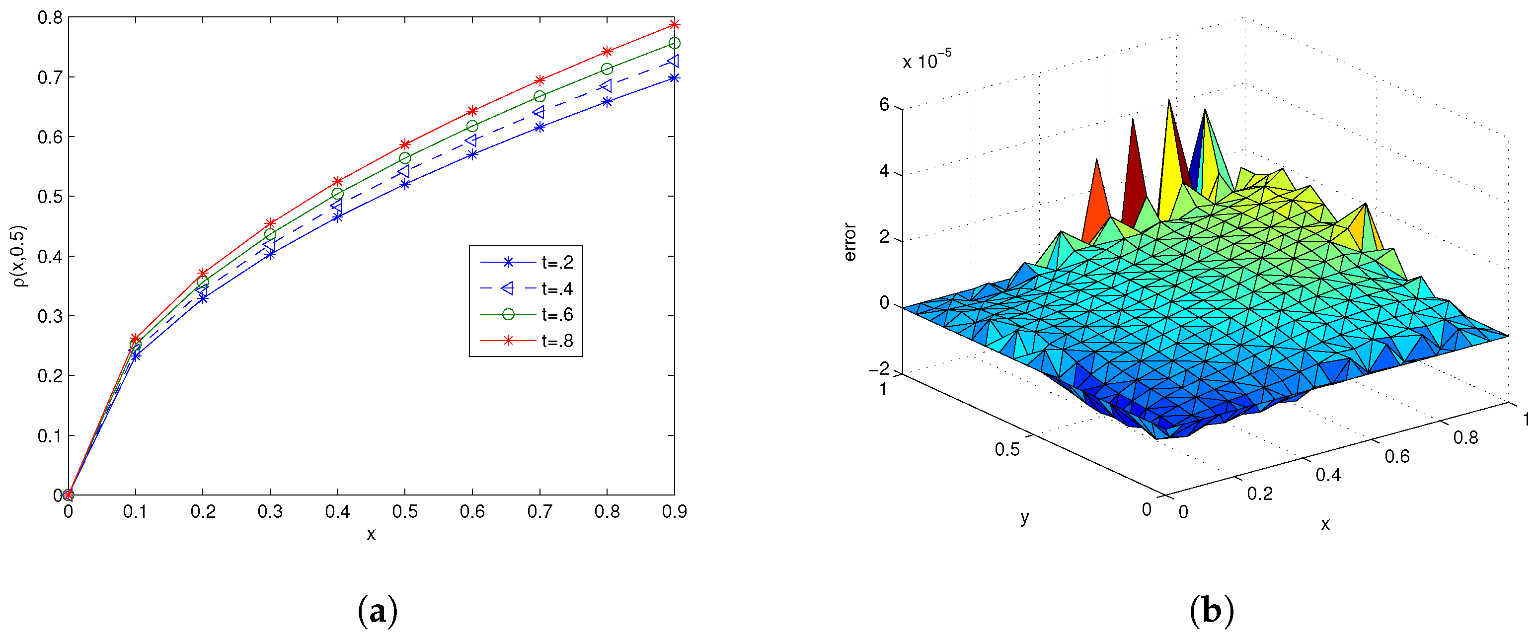
The present problem is solved by the proposed method in the square domain Ω = [ 0 , 1 ] 2 for various number of nodes in the global domain Ω and local sub-domains Ω i . For time integration, the RK4 method with time step δ t = 0.0001 is used. The sparsity of differentiation matrix W and distribution of nodes in the global and local sub-domains corresponding to an interior and boundary points are shown in Figure 1. Figure 2 shows the point wise error and Figure 3 shows the problem solution ρ ( x , 0.5 ) at different times. The results for M = 400 total number of nodes in the global domain, different stencil size n s of local sub-domain, matrix condition number (MCN) and shape parameter are shown in Table 1. The comparison of our method is made with the results in [5] in Table 2, which shows that our results are more accurate and stable.

3.2. Example 2

The biological population model defined by (1) with the initial condition
ρ ( x , y , 0 ) = 1 4 2 x 2 + 2 y 2 + y + 5 ,
with the parameters values h = 1 96 , α = 1 , h = 48 and β = 1 . The exact solution of this problem given in [6] is
ρ ( x , y , t ) = 1 4 2 x 2 + 2 y 2 + y + t 3 + 5 .
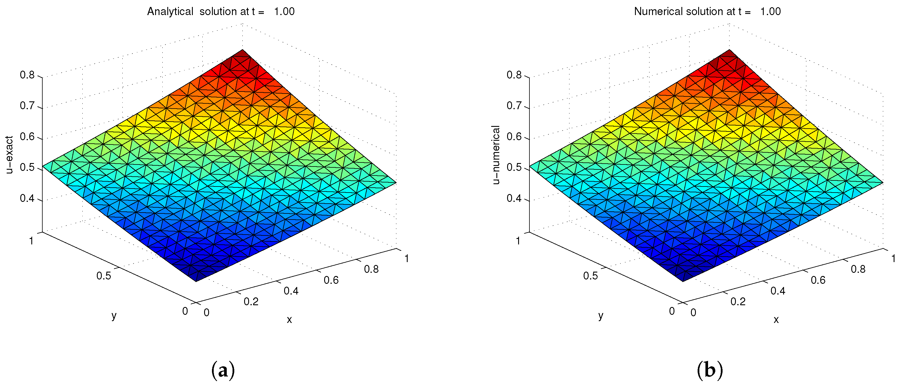
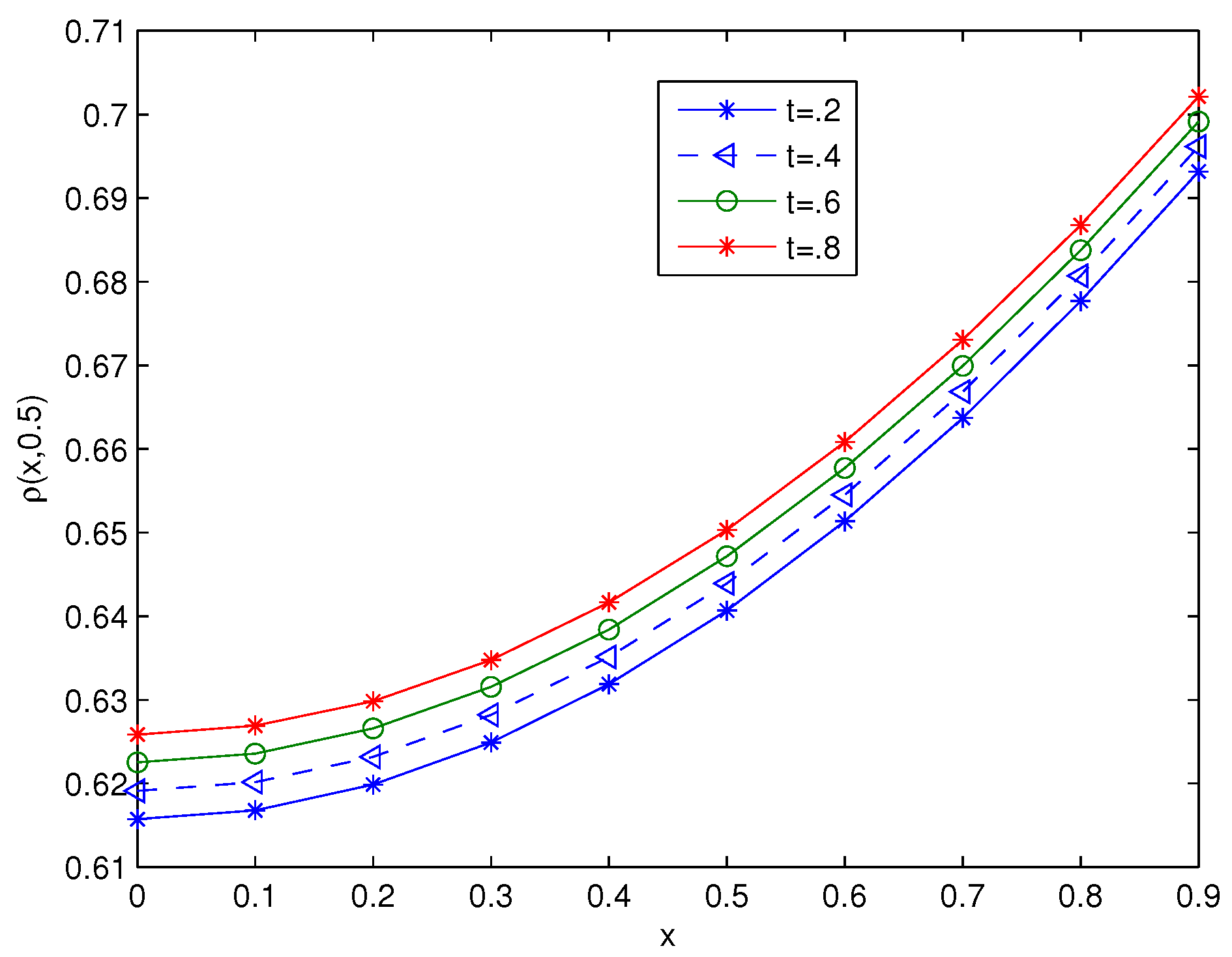
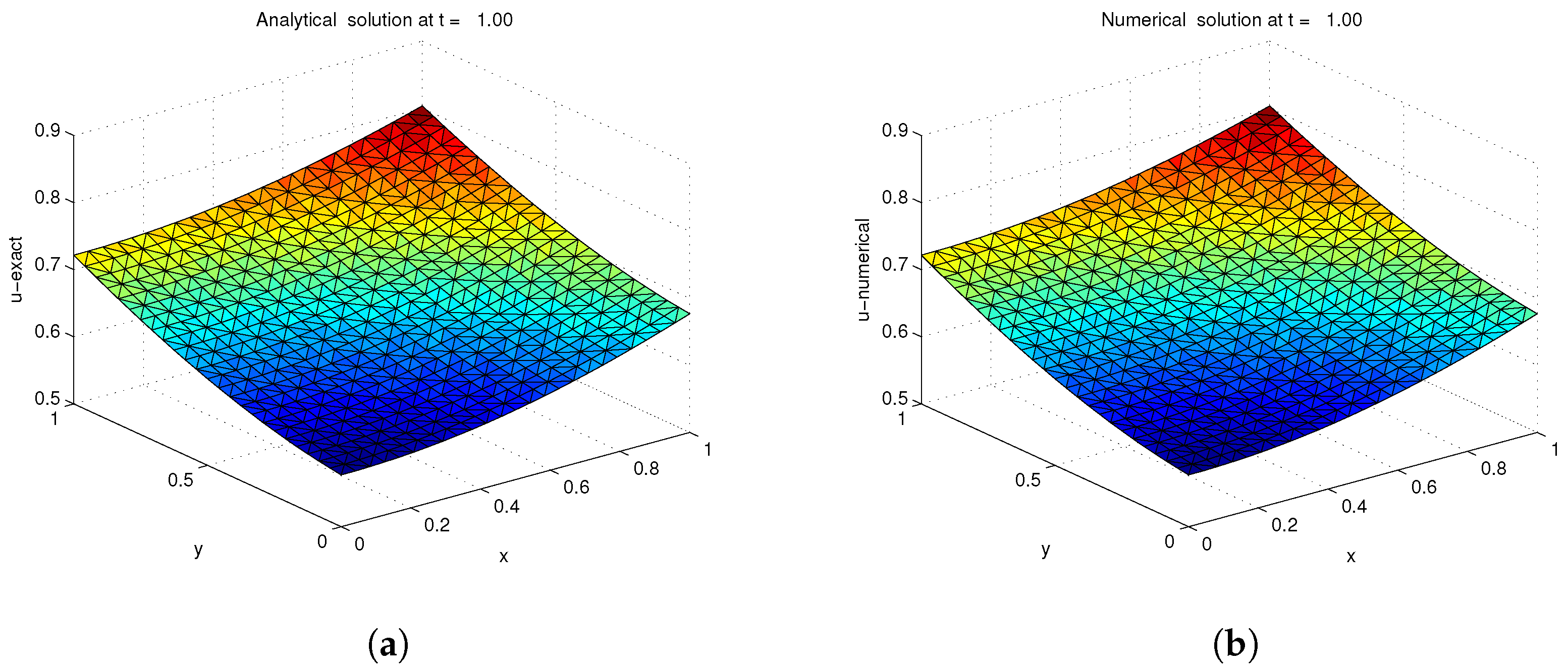
The problem is solved in the square domain Ω = [ 0 , 1 ] 2 , the numerical scheme is advanced in time with step size δ t = 0.0001 . Figure 4 compares the exact and numerical solutions and Figure 5 shows the problem solution ρ ( x , 0.5 ) at different times.

3.3. Example 3

The biological population model defined by (1) with initial condition
ρ ( x , y , 0 ) = e x + y 3 ,
with the values of parameters h = 1 , α = 1 , h = 8 9 and β = 1 . The exact solution [6] is given by
ρ ( x , y , t ) = e x + y 3 t .
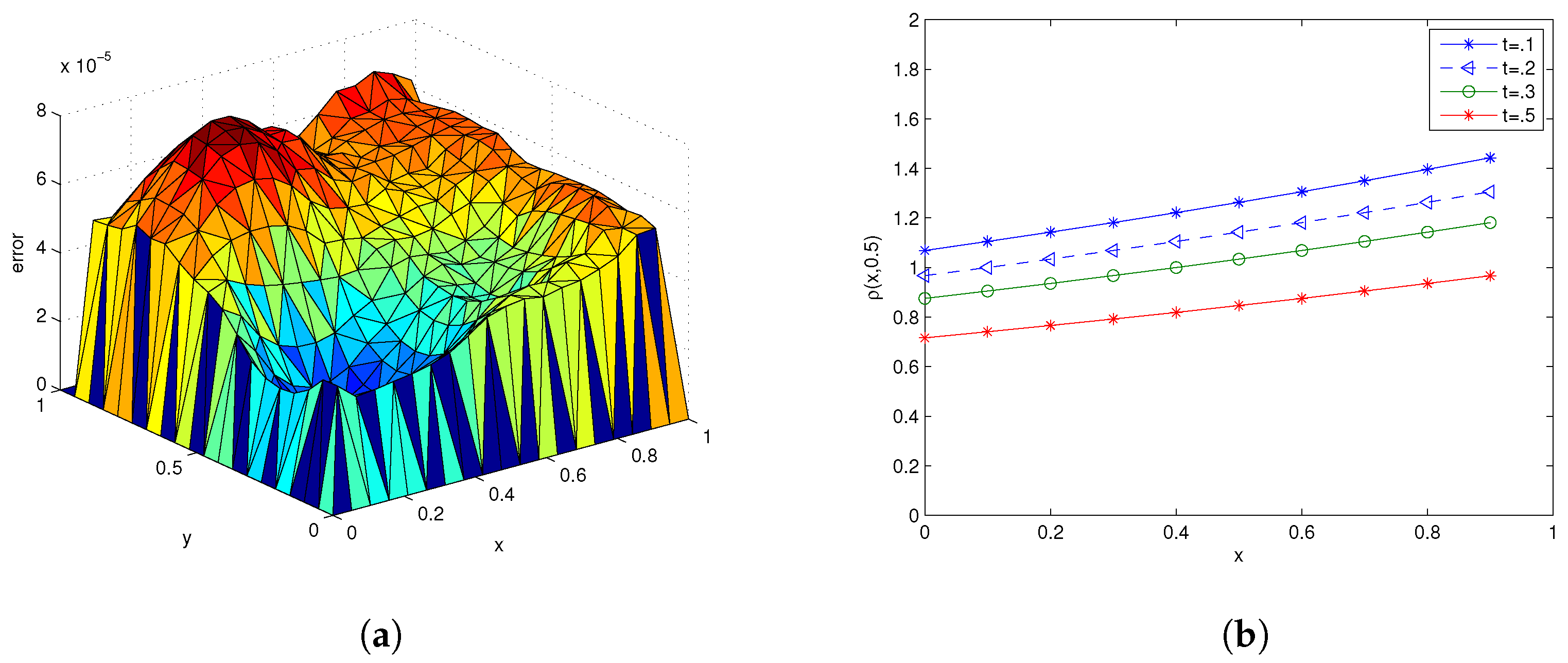
The results are obtained by the present local kernel based method in the domain [ 0.1 ] 2 . Figure 6 compares the exact and numerical solution and Figure 7 shows the point wise error and the model solution ρ ( x , 0.5 ) at different times. The results for different M and n s are obtained and the matrix condition number MCN and shape parameter c are shown in Table 3. The comparison of the present method is made with [5] in Table 4.

3.4. Example 4

In this problem the present method is applied over irregular domains for example Ameoba and Cassini like shaped domains for solving same model discussed in Example 1 above. The parametric equations of such types irregular boundaries Ω are defined as
Ω = { ( x , y ) | x = r ( θ ) cos ( θ ) , y = r ( θ ) sin ( θ ) , 0 θ < 2 π } ,
where for Ameoba-shaped boundary r ( θ ) is defined by
r ( θ ) = e sin ( θ ) sin 2 ( 2 θ ) + e cos θ cos 2 ( 2 θ ) ,
while for Cassini-shaped boundary r ( θ ) is defined by
r ( θ ) = cos ( 4 θ ) + 18 5 sin 2 ( 4 θ ) 3 ,
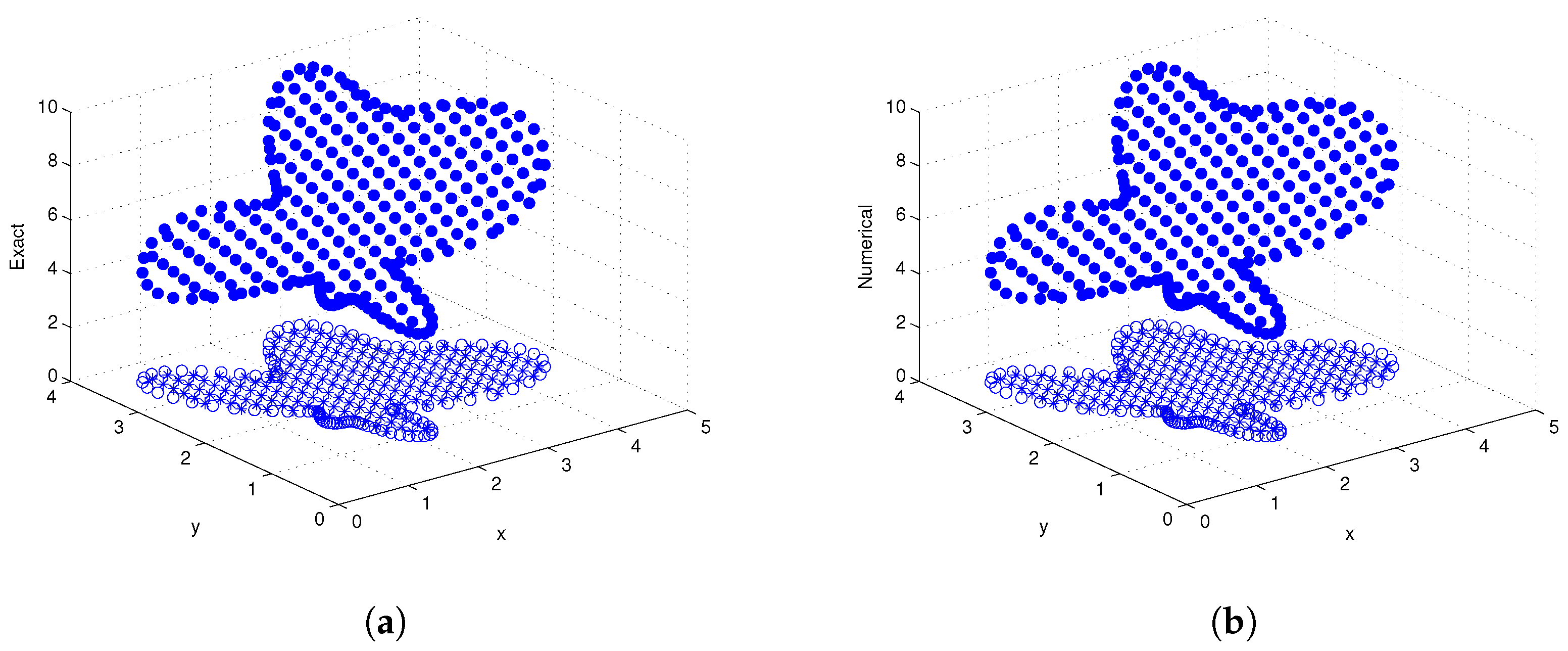
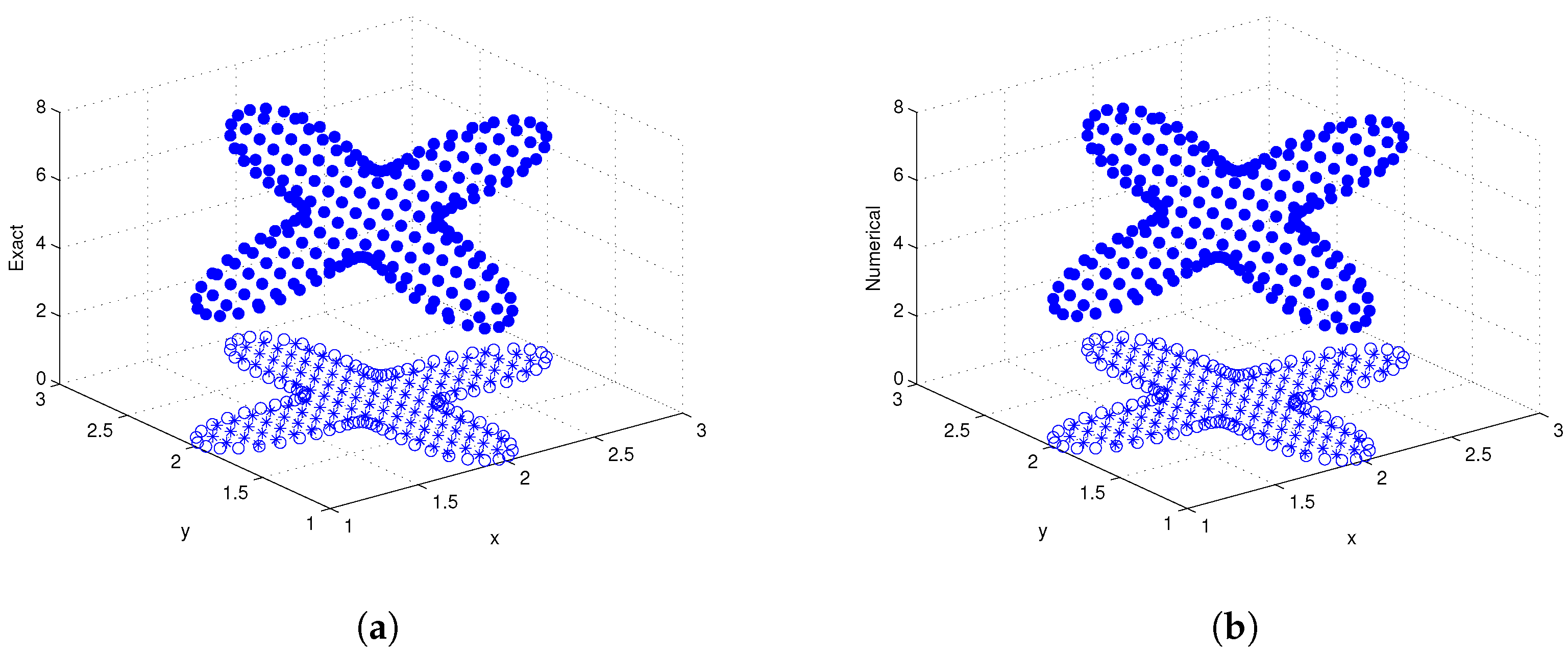
The irregular domains with inner and boundary stencils are shown in Figure 8. The exact and numerical solutions corresponding to Ameoba-like domain with 100 boundary points and Cassini-shape domain with M = 220 are shown in Figure 9 and Figure 10 and Table 5, respectively.

4. Concluding Remarks

In the present paper, the nonlinear biological population model has been numerically simulated using localized RBF method. The multiquadric RBF has been used as the radial kernel. The shape parameter has been chosen using the uncertainty principle. The nonlinear equation is converted to a system of ODEs, which is then advanced in time by the RK4 method. The numerical results are compared with the benchmark problems. The present numerical scheme is more accurate and stable as compared to other numerical methods for solving the biological model considered in this work.

Author Contributions

Investigation, M.U.; Methodology, H.A. and M.T.

Acknowledgments

This work is supported by HEC Pakistan under grant: 112-25237-2PSI-127.

Conflicts of Interest

The authors declare no conflict of interest.

References

  1. Gurtin, M.E.; MacCamy, R.C. On the diffusion of biological populations. Math. Biosci. 1977, 33, 35–49. [Google Scholar] [CrossRef]
  2. Gurney, W.; Nisbet, R. The regulation of inhomogeneous populations. J. Theor. Biol. 1975, 52, 441–457. [Google Scholar] [CrossRef]
  3. Lu, Y.-G. Hölder estimates of solutions of biological population equations. Appl. Math. Lett. 2000, 13, 123–126. [Google Scholar] [CrossRef]
  4. Shakeri, F.; Dehghan, M. Numerical solution of a biological population model using He’s variational iteration method. Comput. Math. Appl. 2007, 54, 1197–1209. [Google Scholar] [CrossRef]
  5. Zhang, L.; Deng, Y.; Liew, K. An improved element-free Galerkin method for numerical modeling of the biological population problems. Eng. Anal. Bound. Elem. 2014, 40, 181–188. [Google Scholar] [CrossRef]
  6. Cheng, R.; Zhang, L.; Liew, K.-M. Modeling of biological population problems using the element-free kp-Ritz method. Appl. Math. Comput. 2014, 227, 274–290. [Google Scholar] [CrossRef]
  7. Golbabai, A.; Seifollahi, S. Numerical solution of the second kind integral equations using radial basis function networks. Appl. Math. Comput. 2006, 174, 877–883. [Google Scholar] [CrossRef]
  8. Golbabai, A.; Seifollahi, S. Radial basis function networks in the numerical solution of linear integro-differential equations. Appl. Math. Comput. 2007, 188, 427–432. [Google Scholar] [CrossRef]
  9. Chen, W. New RBF collocation methods and kernel RBF with applications. In Meshfree Methods for Partial Differential Equations; Springer: Berlin/Heidelberg, Germany, 2003; pp. 75–86. [Google Scholar]
  10. Monaghan, J.J. An introduction to SPH. Comput. Phys. Commun. 1988, 48, 89–96. [Google Scholar] [CrossRef]
  11. Gu, L. Moving kriging interpolation and element-free Galerkin method. Int. J. Numer. Methods Eng. 2003, 56, 1–11. [Google Scholar] [CrossRef]
  12. Atluri, S.N.; Zhu, T. A new meshless local Petrov–Galerkin (MLPG) approach in computational mechanics. Comput. Mech. 1998, 22, 117–127. [Google Scholar] [CrossRef]
  13. Hardy, R.L. Multiquadric equations of topography and other irregular surfaces. J. Geophys. Res. 1971, 76, 1905–1915. [Google Scholar] [CrossRef]
  14. Duchon, J. Splines minimizing rotation-invariant semi-norms in Sobolev spaces. In Constructive Theory of Functions of Several Variables; Springer: Berlin/Heidelberg, Germany, 1977; pp. 85–100. [Google Scholar]
  15. Kansa, E.J. Multiquadrics—A scattered data approximation scheme with applications to computational fluid-dynamics—II solutions to parabolic, hyperbolic and elliptic partial differential equations. Comput. Math. Appl. 1990, 19, 147–161. [Google Scholar] [CrossRef]
  16. Buhmann, M.D. Radial Basis Functions: Theory and Implementations; Cambridge University Press: Cambridge, UK, 2003; Volume 12. [Google Scholar]
  17. Wendland, H. Piecewise polynomial, positive definite and compactly supported radial functions of minimal degree. Adv. Comput. Math. 1995, 4, 389–396. [Google Scholar] [CrossRef]
  18. Fasshauer, G.E. Solving partial differential equations by collocation with radial basis functions. In Proceedings of Chamonix; Vanderbilt University Press: Nashville, TN, USA, 1996; Volume 1997, pp. 1–8. [Google Scholar]
  19. Fasshauer, G.E. Solving differential equations with radial basis functions: Multilevel methods and smoothing. Adv. Comput. Math. 1999, 11, 139–159. [Google Scholar] [CrossRef]
  20. Brown, D.; Ling, L.; Kansa, E.; Levesley, J. On approximate cardinal preconditioning methods for solving PDEs with radial basis functions. Eng. Anal. Bound. Elem. 2005, 29, 343–353. [Google Scholar] [CrossRef]
  21. Uddin, M.; Minullah, Z.; Ali, A. On the approximation of rapidly oscillatory Hankel transform via radial kernels. Dolomites Res. Notes Approx. 2018, 11, 1. [Google Scholar]
  22. Uddin, M.; Ali, H.; Ali, A. Kernel-based local meshless method for solving multi-dimensional wave equations in irregular domain. Comput. Model. Eng. Sci. 2015, 107, 463–479. [Google Scholar]
  23. Uddin, M.; Ali, H. The space–time kernel-based numerical method for Burgers’ equations. Mathematics 2018, 6, 212. [Google Scholar] [CrossRef]
  24. Bianca, C.; Pappalardo, F.; Pennisi, M.; Ragusa, M. Persistence analysis in a Kolmogorov-type model for cancer-immune system competition. AIP Conf. Proc. 2013, 1558, 1797–1800. [Google Scholar]
  25. Barbagallo, A.; Ragusa, M.A. On Lagrange duality theory for dynamics vaccination games. Ricerche di Matematica 2018, 67, 969–982. [Google Scholar] [CrossRef]
  26. Schaback, R.; Wendland, H. Adaptive greedy techniques for approximate solution of large RBF systems. Numer. Algorithms 2000, 24, 239–254. [Google Scholar] [CrossRef]
  27. Shcherbakov, V.; Larsson, E. Radial basis function partition of unity methods for pricing vanilla basket options. Comput. Math. Appl. 2016, 71, 185–200. [Google Scholar] [CrossRef]
  28. Hon, Y.; Schaback, R.; Zhou, X. An adaptive greedy algorithm for solving large RBF collocation problems. Numer. Algorithms 2003, 32, 13–25. [Google Scholar] [CrossRef]
  29. Kosec, G.; Sarler, B. Local RBF collocation method for Darcy flow. Comput. Model. Eng. Sci. 2008, 25, 197. [Google Scholar]
  30. Shu, C.; Ding, H.; Chen, H.; Wang, T. An upwind local RBF-DQ method for simulation of inviscid compressible flows. Comput. Methods Appl. Mech. Eng. 2005, 194, 2001–2017. [Google Scholar] [CrossRef]
  31. Fan, C.-M.; Chien, C.-S.; Chan, H.-F.; Chiu, C.-L. The local RBF collocation method for solving the double-diffusive natural convection in fluid-saturated porous media. Int. J. Heat Mass Transf. 2013, 57, 500–503. [Google Scholar] [CrossRef]
  32. Dormand, J.R.; Prince, P.J. A family of embedded Runge–Kutta formulae. J. Comput. Appl. Math. 1980, 6, 19–26. [Google Scholar] [CrossRef]
  33. Uddin, M. RBF-PS scheme for solving the equal width equation. Appl. Math. Comput. 2013, 222, 619–631. [Google Scholar] [CrossRef]
  34. Nie, Q.; Zhang, Y.-T.; Zhao, R. Efficient semi-implicit schemes for stiff systems. J. Comput. Phys. 2006, 214, 521–537. [Google Scholar] [CrossRef]
  35. Beylkin, G.; Keiser, J.M.; Vozovoi, L. A new class of time discretization schemes for the solution of nonlinear PDEs. J. Comput. Phys. 1998, 147, 362–387. [Google Scholar] [CrossRef]
  36. Uddin, M. On the selection of a good value of shape parameter in solving time-dependent partial differential equations using RBF approximation method. Appl. Math. Model. 2014, 38, 135–144. [Google Scholar] [CrossRef]
  37. Schaback, R. Error estimates and condition numbers for radial basis function interpolation. Adv. Comput. Math. 1995, 3, 251–264. [Google Scholar] [CrossRef]
Figure 1. (a) Sparsity of matrix W, when n s = 30 and M = 400 , and (b) centre distribution in domain [ 0 , 1 ] 2 corresponding to Example 1.
Mca 24 00054 g001
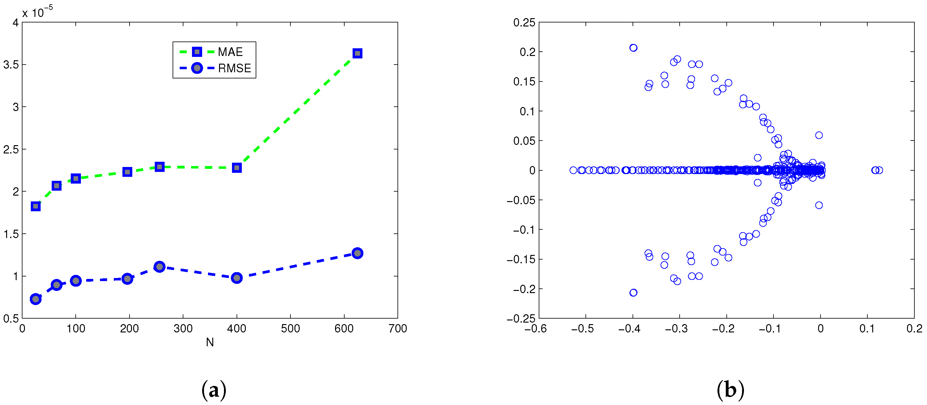
Figure 2. (a) Nodes M against MAE and RMSE norms for n s = 20 , and (b) stability plots of our numerical scheme corresponding to Example 1.
Mca 24 00054 g002
Figure 3. (a) Numerical solution ρ ( x , 0.5 ) at different times t, and (b) point wise error when t = 1 , n s = 20 and δ = 0.0001 when M = 400 corresponding to Example 1.
Mca 24 00054 g003
Figure 4. (a) Exact against (b) numerical solutions, when t = 1 , δ t = 0.0001 , n s = 20 , M = 400 , corresponding to Example 2.
Mca 24 00054 g004
Figure 5. Numerical solution at different times t for ρ ( x , 0.5 ) , corresponding to Example 2.
Mca 24 00054 g005
Figure 6. (a) Exact against (b) numerical solutions, when t = 1 , δ t = 0.0001 , n s = 20 , M = 400 corresponding to Example 3.
Mca 24 00054 g006
Figure 7. (a) Point wise error, when t = 1 , n s = 20 and δ t = 0.0001 , and (b) numerical solution, corresponding to Example 3.
Mca 24 00054 g007
Figure 8. (a) Ameoba and (b) Cassini-shaped domain with interior (red) and boundary (green) stencil.
Mca 24 00054 g008
Figure 9. (a) Exact against (b) numerical solution of Ameoba-shaped domain when t = 1 , δ t = 0.0001 , n s = 10 , M = 291 to Example 4.
Mca 24 00054 g009
Figure 10. (a) Exact against (b) numerical solution of Cassini-shaped domain when t = 1 , δ t = 0.0001 , n s = 10 , M = 220 to Example 4.
Mca 24 00054 g010
Table 1. Numerical results when N = 400 for domain [ 0 , 1 ] 2 (Example 1).
nsMCNMAERMSEC-TimeShape (c)
RK4 (MQ RBF)53.099 × 10 14 1.931 × 10 5 8.336 × 10 6 0.9500.010
111.241 × 10 13 1.915 × 10 5 7.935 × 10 6 0.8580.520
217.732 × 10 13 1.215 × 10 5 7.643 × 10 6 2.3191.160
492.929 × 10 14 4.109 × 10 5 1.269 × 10 5 1.8691.990
602.941 × 10 14 2.725 × 10 5 1.121 × 10 5 2.5042.150
805.096 × 10 14 2.961 × 10 5 1.287 × 10 5 4.1992.320
Table 2. Numerical solution of ρ ( x , y , t ) at x = 0.5 , y = 0.5 compared with exact solution and Zhang et al. [5] (Example 1).
Number of Nodes = 13 × 13 t = 0.1 t = 0.2 t = 0.3 t = 0.4 t = 0.5
Present Solution1.26281.14261.03390.93550.8465
Zhang et al. Solution [5]1.25741.13821.03020.93250.844
Exact Solution1.26281.14261.03390.93550.8465
Table 3. Numerical results corresponding to Example 3 in [ 0 , 1 ] 2 .
nsMCNMAERMSEC-TimeShape (c)
RK4 (MQ RBF)53.099 × 10 14 1.35 × 10 4 8.85 × 10 5 0.145380.01
105.136 × 10 13 6.93 × 10 5 4.70 × 10 5 0.769460.43
154.549 × 10 13 6.90 × 10 5 4.75 × 10 5 0.777730.85
251.367 × 10 14 7.50 × 10 5 5.47 × 10 5 0.886581.41
503.225 × 10 14 7.34 × 10 5 4.67 × 10 5 1.265771.99
703.558 × 10 14 6.92 × 10 5 4.72 × 10 5 1.572712.26
805.096 × 10 14 7.53 × 10 5 4.53 × 10 5 1.742312.32
Table 4. Numerical solution of ρ ( x , y , t ) at x = 0.5 , y = 0.5 compared with exact solution and Zhang et al. [5] (Example 3).
Number of Nodes = 13 × 13 t = 0.1 t = 0.2 t = 0.3 t = 0.4 t = 0.5
Present Solution1.26281.14261.03390.93550.8465
Zhang et al. Solution [5]1.25741.13821.03020.93250.844
Exact Solution1.26281.14261.03390.93550.8465
Table 5. MAE and RMSE for Ameoba and Cassini-shaped domains at t = 1 with different stencil sizes.
AmeobaCassini
nsMAERMSEMAERMSE
59.40 × 10 4 3.52 × 10 4 1.63 × 10 4 1.02 × 10 4
152.40 × 10 4 2.21 × 10 4 7.33 × 10 4 4.32 × 10 4
303.20 × 10 3 9.12 × 10 3 6.36 × 10 4 3.82 × 10 4
451.78 × 10 4 1.51 × 10 4 2.51 × 10 4 1.56 × 10 4
601.20 × 10 4 2.12 × 10 4 4.45 × 10 4 2.22 × 10 4