A Tutorial for the Analysis of the Piecewise-Smooth Dynamics of a Constrained Multibody Model of Vertical Hopping

Abstract

Contradictory demands are present in the dynamic modeling and analysis of legged locomotion: on the one hand, the high degrees-of-freedom (DoF) descriptive models are geometrically accurate, but the analysis of self-stability and motion pattern generation is extremely challenging; on the other hand, low DoF models of locomotion are thoroughly analyzed in the literature; however, these models do not describe the geometry accurately. We contribute by narrowing the gap between the two modeling approaches. Our goal is to develop a dynamic analysis methodology for the study of self-stable controlled multibody models of legged locomotion. An efficient way of modeling multibody systems is to use geometric constraints among the rigid bodies. It is especially effective when closed kinematic loops are present, such as in the case of walking models, when both legs are in contact with the ground. The mathematical representation of such constrained systems is the differential algebraic equation (DAE). We focus on the mathematical analysis methods of piecewise-smooth dynamic systems and we present their application for constrained multibody models of self-stable locomotion represented by DAE. Our numerical approach is demonstrated on a linear model of hopping and compared with analytically obtained reference results.

1. Introduction

1.1. Background

Many descriptive models of legged locomotion—such as walking, running, and hopping—can be found in the literature. These descriptive models are mainly capable of interpreting measurement results on walking, running, and hopping [1,2,3,4,5,6,7].

Alternative modeling approaches do not necessitate the experimental results, but develop predictive models, which imitate the dynamics of locomotion. For instance, references [8,9] introduce models for the investigation of foot impact intensity at forefoot, mid-foot and rear-foot ground collision. In [10], the geometric non-linearity of a static segmented leg model is studied. The SLIP model in [11] has been developed for the understanding of the essential dynamics of running and hopping locomotion. The further detailed variation of the SLIP model is presented in [12]: the segmented leg provides a geometry very similar to the human leg; however, the inertia of leg segments is neglected; consequently, the ground-foot collision and the impact-induced energy absorption are not investigated. Reference [13] introduces a novel approach for humanoid gait generation. The control of foot placement and human balancing problems are discussed in [14], where a predictive model is applied.

Our research contributes to the development of mathematical models of legged locomotion. Since the mathematical description of the above-mentioned and the similar predictive models are quite challenging, these models develop slowly, and the integration of the features leads to highly intricate mathematical description. The long-term goal of our research is to reach such integrated models of hopping and running that can analyze (i) the dynamic stability issues, the neural processes such as balancing [14,15,16,17], the motion control and the motion pattern generation [18]; (ii) geometric non-linearities [10,12,19,20]; (iii) ground-foot collision intensity and impact-induced energy absorption [9,21,22]; (iv) distinct topology and actuation in the flight and ground phases [23].

In paper [24], we introduced a simple 2 DoF model of hopping that demonstrated how the active control provides stable hopping with uniform hopping height despite of the impact-induced energy absorption. The model consists of two mass blocks one above the other and connected to each other by means of an active spring-damper. In [24], we demonstrated a general dynamic analysis method, which is suitable for more complex models, such as the 6 DoF model in [20]. The analysis of the three-segmented hopping model in [20] is based on the dynamic analysis method explained in [24] and demonstrates the applicability for higher DoF systems.

The present paper introduces and overview a dynamic analysis methodology which is suitable for higher complexity multibody models. The mathematical representation of the models in [20,24] are based on the classical general coordinates of the minimum set. However, in the case of high number of DoF or closed kinematic loops, the application of non-minimum set (also referred as redundant set) of descriptor coordinates is more efficient. The application of non-minimum coordinates in multibody dynamics is well known from [25,26,27,28,29,30]. In case on non-minimal coordinates, the dynamic equation of motion is subjected to algebraic constraint equations that assure the geometric connection of the redundant coordinates. The constrained representation of the equations of motion suits well the possibly intricate combination of ground-foot contacts and makes possible to analyze models when more than one leg can touch the ground. This technique leads to the situation, when the equation of motion has DAE form. In the present work, we combine the stability analysis method of the periodic solution of piecewise-smooth dynamic systems that are described by ordinary differential equations (ODE) [21,31,32,33] with the efficient DAE formulation of multibody systems [25,27,34] and legged locomotion systems [28,30]. The fundamental theories and ideas of the analysis of the legged locomotion with similar approaches are detailed in [35]. The applied dynamic analysis technique is specialization of the method in [36] for hopping and running multibody models.

1.2. Organization of the Paper

Our models of vertical hopping with coordinates of minimum set and redundant set are detailed in Section 2. The models consist of the equation of motion of the mechanical system and the equations of the control actions. Section 3 details the dynamic analysis method, which is specifically tailored for non-linear hopping and running systems with redundant coordinates and two continuous phases. The numerical results together with their analytical validation are presented in Section 4. The analytical calculation exploits the fact that the model is linear; however, it is not a requirement for the presented numerical dynamic analysis method. The conclusions are summarized in Section 5.

2. A Constrained Model of Vertical Hopping

The DAE-based dynamic analysis methodology of piecewise-smooth hopping and running systems is presented by the case study of an excessively simplified model of hopping. Hence, we can rather focus on the analysis methodology.

For the sake of simplicity, a constrained linear model of hopping is introduced in this section. However, non-linearities may emerge in locomotion models due to geometric non-linearities, such as in case the model in [37]; spring characteristics due to the muscle-tendon dynamics [10]; or non-linear behavior of the neural model [11]. Although these non-linearities do not appear in our basic hopping model, the dynamic analysis method is not limited to linear systems.

2.1. Mechanical Model

Our simplest hopping models consist of two vertically moving particles connected by an active spring-damper. The model is placed in gravitational field above smooth, rigid, and horizontal ground. The constrained model, which is shown in the right panel of Figure 1, has been developed based on the unconstrained hopping model that was published in [24] and is shown in Figure 1 left. The unconstrained model in [24] and our new model match each other in terms of physical parameters and DoF. The difference is the mathematical representation: the upper and lower body has been split into two parts and constrained to each other in the new model. The constrained model on the right panel of Figure 1 is used as a case example to illustrate our analysis methodology; however, the presented methodology is suitable for multibody models with high complexity.

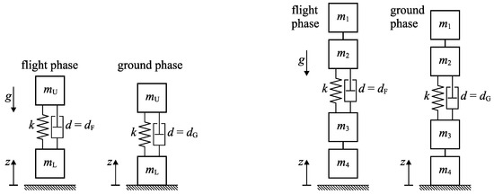
Figure 1. The unconstrained hopping model in the flight and the ground phases [24] (left panel); the constrained model in the flight and the ground phases (right panel)

Similarly to the unconstrained model, the physical parameters are the total mass m and the ratio $\mu \in [0,1]$ of the upper and lower mass. The upper $m_{\mathrm{U}}$ and lower masses $m_{\mathrm{L}}$ are further separated by means of parameters ${\mu }_{\mathrm{U}}\in [0,1]$ and ${\mu }_{\mathrm{L}}\in [0,1]$, with which

$$m_1=m_{\mathrm{U}}{\mu }_{\mathrm{U}},$$

(1)

$$m_2=m_{\mathrm{U}}(1-{\mu }_{\mathrm{U}}),$$

(2)

$$m_3=m_{\mathrm{L}}{\mu }_{\mathrm{L}},$$

(3)

$$m_4=m_{\mathrm{L}}(1-{\mu }_{\mathrm{L}}),$$

(4)

where

$$m_U=m\mu ,$$

(5)

$$m_L=m(1-\mu )$$

(6)

are the mass of the upper and lower blocks in the unconstrained model. Further parameters of the model are the stiffness k and the damping parameters $d_{\mathrm{F}}$ and $d_{\mathrm{G}}$, which are valid in flight and ground phases, respectively. For the better interpretation of the results (in Section 4) and in order to reduce the number of parameters, we introduce $\alpha =\sqrt{k/m}$, $D_{\mathrm{F}}=d_{\mathrm{F}}/\left(2\alpha m\right)$ and $D_{\mathrm{G}}=d_{\mathrm{G}}/\left(2\alpha m\right)$.

The system is described by the non-minimum set of coordinates $\mathbf{q}={[z_1\left(t\right),z_2\left(t\right),z_3\left(t\right),z_4\left(t\right)]}^{\mathrm{T}}$ of the number of $n=4$, and the following geometric constraints ensure the connection of the descriptor coordinates:

$${\gamma }_{\mathrm{b}}=\left[\begin{array}{c}{z}_1-z_2\\ z_3-z_4\end{array}\right].$$

(7)

The rigid body constraints in ${\gamma }_{\mathrm{b}}$ are permanently valid in both the flight and the ground phases. The number of permanent rigid body constraints is $h=2$ in our case example. In the case of this hopping model, ${\gamma }_{\mathrm{b}}$ is linear. However, it is not a requirement for the general formalism detailed in Section 3.2.

In the specific case of our hopping model, the number of constraints that represent ground contact is $l=1$, and the corresponding constraint vector is

$${\gamma }_{\mathrm{g}}=\left[\begin{array}{c}{z}_4\end{array}\right].$$

(8)

Again, in the case of our model, ${\gamma }_{\mathrm{g}}$ is linear too, which is not a requirement for the general formalism detailed in Section 3.2.

To construct the equation of motion, we derive the mass matrix $\mathbf{H}$ and the vector $\mathbf{C}$ of spring, damping and gravitational forces, which are

$$\mathbf{H}=\mathrm{diag}\left(\left[\begin{array}{cccc}{m}_1,& m_2,& m_3,& m_4\end{array}\right]\right),$$

(9)

$$\mathbf{C}=\left[\begin{array}{c}0\\ k(z_2-z_3-L_0)+d({\dot{z}}_2-{\dot{z}}_3)\\ -k(z_2-z_3-L_0)-d({\dot{z}}_2-{\dot{z}}_3)\\ 0\end{array}\right]+g\left[\begin{array}{c}{m}_1\\ m_2\\ m_3\\ m_4\end{array}\right],$$

(10)

where $L_0$ is the unstretched spring length. The general force vector $\mathbf{C}$ in (10) and the mass matrix in $\mathbf{H}$ (9) are linear and constant, respectively. However, $\mathbf{C}$ and $\mathbf{H}$ can be non-linear functions of the state variables in the general formalism (Section 3.2).

2.2. Active Spring-Damper for Ensuring Periodic Motion

The flight (airborne) phase and ground (support or stance) phases, which periodically follow each other, are clearly separated in our models. In such systems, some segments of the limbs periodically come into contact with the ground; therefore, the motion of these body segments are constrained during the whole duration of the ground contact. The ground collision at the end of the flight phase leads to the loss of a certain amount of kinetic energy [9,11,21,24]. This energy amount is referred as constraint motion space kinetic energy (CMSKE) in [22]. As the muscles or actuators provide mechanical power, the kinetic energy accumulates in the rest of the body during the ground phase. In the case of periodic motion, the mechanical energy reaches its original level at the end of the ground phase. The ground contact then terminates, and the flight phase begins again.

The unconstrained model, which is depicted in the left panel of Figure 1, is developed for the illustration and dynamic analysis of the above explained sequence. The ground collision of $m_{\mathrm{L}}$ terminates the flight phase and the total amount of the kinetic energy of $m_{\mathrm{L}}$ is absorbed, since the collision is modeled to be fully inelastic. The active spring-damper plays the role of the muscles: it accelerates $m_{\mathrm{U}}$ in upward vertical direction and increases its kinetic energy. If the height of the new hop is the same as it was in the previous one, then the motion is periodic.

We can conclude that hopping systems with collisions are non-conservative without active control. This issue and the modeling of energy supply are thoroughly surveyed in [11]. A specific concept for the energy refilling of impacting hopping systems is presented in the case of a general 1 DoF non-linear model of hopping presented in [38]. Since the damper and the spring is linear in our model, it is more specific. Having linear dynamics allows us to carry out analytical calculations, with which the numerically obtained results are validated (see Section 4.1). Besides, the presented numerical analysis is not limited to linear systems.

The active spring-damper system imitates the behavior of limb muscles in the sense that muscles supply energy lost to dissipation and foot impacts according to [11,38]. The spring-damper plays different role in the flight and the ground phases. The damper d has a certain positive value $d_{\mathrm{F}}$ in the flight phase to suppress undesired oscillations. However, it has a properly chosen negative value $d_{\mathrm{G}}$ in ground phase to regenerate mechanical energy. The negative damping could be achieved by means of an active actuator in a robotic realization of the model. The stiffness k is constant regardless the variation of the flight and the ground phases. The operation of the active spring-damper system is the same in the constrained model.

2.3. Switchings between the Flight and the Ground Phases

As we explained in Section 2.2, the flight phase terminates when the mass block in the lowest position reaches the ground. The event of flight to ground (F2G) transition is mathematically expressed by means of the indicator function $h_{\mathrm{F}2\mathrm{G}}\in \mathbb{R}$:

$$\begin{array}{c}\hfill h_{\mathrm{F}2\mathrm{G}}\left(\mathbf{x}\right)=z_4.\end{array}$$

(11)

The indicator function $h_{\mathrm{F}2\mathrm{G}}$ crosses zero from positive to negative direction at touchdown. The F2G transition not only cause the switching of the governing equation of the continuous dynamics, but involves an impact too. The impact is modeled as a mapping (i.e., resetting) of the state variables: the velocity of the lower mass blocks becomes zero and other state variables remain the same. The mapping is defined as

$$\begin{array}{c}\hfill {\mathbf{g}}_{\mathrm{F}2\mathrm{G}}\left(\mathbf{x}\right)={[\mathbf{q},{\dot{z}}_1,{\dot{z}}_2,0,0]}^{\mathrm{T}}.\end{array}$$

(12)

The ground to flight (G2F) transition occurs, when the ground-foot force becomes a pulling force. Mathematically, the G2F transition occurs, when indicator function

$$\begin{array}{c}\hfill h_{\mathrm{G}2\mathrm{F}}\left(\mathbf{x}\right)={\lambda }_{\mathrm{g}}\end{array}$$

(13)

crosses zero from negative to positive direction. The Lagrange-multiplier ${\lambda }_{\mathrm{g}}$ in $h_{\mathrm{G}2\mathrm{F}}\in \mathbb{R}$ is the ground contact force acting on particle $m_4$. Negative and positive sign of ${\lambda }_{\mathrm{g}}$ refers to pushing and pulling force, respectively. The mapping after ground-foot release is identity, since the state variables does not change. This type of transition characterizes the Filippov systems [31,39]. The mapping is defined by

$$\begin{array}{c}\hfill {\mathbf{g}}_{\mathrm{G}2\mathrm{F}}\left(\mathbf{x}\right)={[\mathbf{q},\dot{\mathbf{q}}]}^{\mathrm{T}}.\end{array}$$

(14)

3. Dynamic Analysis

The analysis methods of the periodic solutions of hybrid systems, which are described by minimum coordinates, are detailed in [21,31,32,39]. In particular, the analysis and control of the local stability of periodic orbits of hybrid systems is detailed in [32]. A constrained formalism for the analysis of legged locomotion systems is developed in [28,30]. The general analysis of piecewise constrained systems is detailed in [36]. The formalism is particularly efficient when intricate combination of ground-limb contact emerges. Our contribution is in the application of the stability analysis method in multibody models of hopping and running systems in constrained mathematical representation. Furthermore, the method is demonstrated on an illustrative case example of a simple hopping system.

3.1. Assumptions and Limitations

We focus on hopping or running motion only, when the limb(s) that periodically touches the ground has a larger than zero elevation in the flight phase. Accordingly, motion types with continuous ground contact are out of scope in this work. We assume that (a) the flight phase and the ground phase periodically switch each other. This assumption helps to avoid the consideration of intricate combinations of the sequence of various dynamics, which may happen e.g., in the case of more than one limb.

Furthermore, we assume that (b) the ground-foot collision is instantaneous, which leads to infinitely large instantaneous forces over infinitesimal time duration so that the net impulse due to the impact force is finite [8,9,22]. Additionally, (c) completely inelastic collision is assumed, hence there is no rebound [8,22]. Assumption (d) is that there is no slip (more details in Section 3.2). Assumptions (b), (c) and (d) allows us to consider the ground-foot contact as an instantly arising geometric constraint such as in [1,9,22,40,41,42].

3.2. Continuous Dynamics in the Flight and in the Ground Phases

The general form of the equation of motion is a DAE, since the dynamic Equations (15) are augmented with the algebraic equations that represent geometric constraints (16):

$$\mathbf{H}\left(\mathbf{q}\right)\ddot{\mathbf{q}}+\mathbf{C}(\mathbf{q},\dot{\mathbf{q}})+{\gamma }_{\mathbf{q}}^{\mathrm{T}}\left(\mathbf{q}\right)\mathbf{\lambda }=\mathbf{0},$$

(15)

$$\gamma \left(\mathbf{q}\right)=\mathbf{0},$$

(16)

where the vector $\mathbf{q}$ contains the differential variables and the vector $\mathbf{\lambda }$ contains the algebraic variables. The mass matrix of the unconstrained system is $\mathbf{H}\in {\mathbb{R}}^{n\times n}$, the vector $\mathbf{C}\in {\mathbb{R}}^n$ represents the velocity dependent inertial forces, the forces exerted by springs and dampers, gravitational forces and any active forces in general. The matrix

$$\begin{array}{c}\hfill {\gamma }_{\mathbf{q}}\left(\mathbf{q}\right)=\frac{\partial \gamma \left(\mathbf{q}\right)}{\partial \mathbf{q}}\end{array}$$

(17)

is the gradient of the geometric constraint vector $\gamma$, and $\mathbf{\lambda }$ is the vector of the corresponding Lagrange-multipliers.

The equation of motion (15) together with the geometric constraint Equation (16) are reorganized by means of DAE index reduction, which leads to the following general form used in [25,27,28,30]:

$$\begin{array}{c}\hfill \left[\begin{array}{c}\ddot{\mathbf{q}}\\ \mathbf{\lambda }\end{array}\right]={\left[\begin{array}{cc}\mathbf{H}\left(\mathbf{q}\right)& {\gamma }_{\mathbf{q}}^{\mathrm{T}}\left(\mathbf{q}\right)\\ {\gamma }_{\mathbf{q}}\left(\mathbf{q}\right)& \mathbf{0}\end{array}\right]}^{-1}\left[\begin{array}{c}-\mathbf{Q}\left(\mathbf{q}\right)\\ -{\dot{\gamma }}_{\mathbf{q}}(\mathbf{q},\dot{\mathbf{q}})\dot{\mathbf{q}}\end{array}\right].\end{array}$$

(18)

The form (18) makes possible to express the acceleration $\ddot{\mathbf{q}}\in {\mathbb{R}}^n$ as the function of the state variables, which are collected in $\mathbf{x}={\left[\mathbf{q},\dot{\mathbf{q}}\right]}^{\mathrm{T}}$, where $\mathbf{x}\in {\mathbb{R}}^{2n}$ is the state vector. Finally, the continuous dynamics is governed by

$$\dot{\mathbf{x}}\left(t\right)={\mathbf{f}}_{\mathrm{F}}\left(\mathbf{x}\left(t\right)\right)\mathrm{and}$$

(19)

$$\dot{\mathbf{x}}\left(t\right)={\mathbf{f}}_{\mathrm{G}}\left(\mathbf{x}\left(t\right)\right),$$

(20)

where ${\mathbf{f}}_{\mathrm{F}}\in {\mathbb{R}}^{2n}$ and ${\mathbf{f}}_{\mathrm{G}}\in {\mathbb{R}}^{2n}$ are smooth vector fields corresponding to the flight and the ground phase dynamics, respectively.

The vector field ${\mathbf{f}}_{\mathrm{F}}$ is obtained by using the permanent rigid body constraints ${\gamma }_{\mathrm{b}}\in {\mathbb{R}}^h$ only (for our case example, see (7)). Hence, the entire constraint vector ${\gamma }_{\mathrm{F}}\in {\mathbb{R}}^h$ is the following in the flight phase:

$$\begin{array}{c}\hfill {\gamma }_{\mathrm{F}}={\gamma }_{\mathrm{b}}.\end{array}$$

(21)

The ground-foot contact is modeled by geometric constraints ${\gamma }_{\mathrm{g}}\in {\mathbb{R}}^l$. In our specific case example (8) stands. In the ground phase, the overall constraint vector ${\gamma }_{\mathrm{G}}\in {\mathbb{R}}^{h+l}$, which is incorporated in ${\mathbf{f}}_{\mathrm{G}}$, reads:

$$\begin{array}{c}\hfill {\gamma }_{\mathrm{G}}=\left[\begin{array}{c}{\gamma }_{\mathrm{b}}\\ {\gamma }_{\mathrm{g}}\end{array}\right].\end{array}$$

(22)

Considering a convenient running kinematics, assumption d in Section 3.1 is usually satisfied in practice, since depending on the surface quality, normally there is no significant slip of the foot. Although the slip-free condition is checked in such models, when not only vertical motion is considered, e.g., [19,20]. The ground-foot constraint is separated into two parts: ${\gamma }_{\mathrm{t}}$ and ${\gamma }_{\mathrm{n}}$ respectively constrains the motion in the tangential and in the normal direction relative to the ground surface. The ground-foot constraint reads:

$$\begin{array}{c}\hfill {\gamma }_{\mathrm{g}}=\left[\begin{array}{c}{\gamma }_{\mathrm{t}}\\ {\gamma }_{\mathrm{n}}\end{array}\right]\end{array}$$

(23)

in the frame of the tangential and the normal directions. To satisfy the non-slip condition, the Coulomb friction coefficient must be larger than the critical value [43]:

$$\begin{array}{c}\hfill {\kappa }_{\mathrm{c}}=\left|\frac{{\gamma }_{\mathbf{q},\mathrm{n}}{\mathbf{H}}^{-1}{\gamma }_{\mathbf{q},\mathrm{t}}^{\mathrm{T}}}{{\gamma }_{\mathbf{q},\mathrm{n}}{\mathbf{H}}^{-1}{\gamma }_{\mathbf{q},\mathrm{n}}^{\mathrm{T}}}\right|,\end{array}$$

(24)

where ${\gamma }_{\mathbf{q},\mathrm{t}}$ and ${\gamma }_{\mathbf{q},\mathrm{n}}$ are the Jacobians of constraints ${\gamma }_{\mathrm{t}}$ and ${\gamma }_{\mathrm{n}}$ respectively.

3.3. Piecewise-Smooth Periodic Orbits and Impacts in Hopping and Running

The combined solution $\mathbf{\varphi }({\mathbf{x}}_0,t)$ of (19) and (20) go through the smooth vector fields ${\mathbf{f}}_{\mathrm{F}}$ and ${\mathbf{f}}_{\mathrm{G}}$, which are separated from each other by switching surfaces ${\Sigma }_{\mathrm{F}2\mathrm{G}}$ and ${\Sigma }_{\mathrm{G}2\mathrm{F}}$ as it is shown in Figure 2. Flight to ground (F2G) transition occurs at $t=t_{\mathrm{F}2\mathrm{G}}$, when the switching surface ${\Sigma }_{\mathrm{F}2\mathrm{G}}$, which is defined by the scalar indicator function $h_{\mathrm{F}2\mathrm{G}}\left(\mathbf{x}\right)$, is reached from positive to negative direction. The indicator function $h_{\mathrm{F}2\mathrm{G}}\left(\mathbf{x}\right)$ expresses the relative position of the ground and the end of the limb. After the impact, the solution remains on the ${\Sigma }_{\mathrm{F}2\mathrm{G}}$ switching surface itself in the entire ground phase. Ground to flight (G2F) transition occurs at $t=t_{\mathrm{G}2\mathrm{F}}$, when set ${\Sigma }_{\mathrm{G}2\mathrm{F}}$, which is defined by $h_{\mathrm{G}2\mathrm{F}}\left(\mathbf{x}\right)$ and intersects ${\Sigma }_{\mathrm{F}2\mathrm{G}}$, is crossed from negative to positive direction. Function $h_{\mathrm{G}2\mathrm{F}}\left(\mathbf{x}\right)$ expresses the normal component of the ground contact force. We remark, that the entire period ends at time instant $t_{\mathrm{p}}:=t_{\mathrm{G}2\mathrm{F}}$.

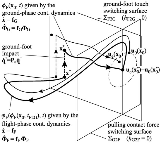
Figure 2. The periodic orbit, the perturbed motion, the switching surfaces, and the discrete mapping at F2G transition.

According to the PhD thesis by [31], piecewise-smooth systems can be classified according to the degree of discontinuity. In the case of the G2F transition, the solution goes through the switching surface ${\Sigma }_{\mathrm{G}2\mathrm{F}}$ without discontinuity (i.e., without mapping or reset of the state variables). Hence, the mapping is an identity:

$$\begin{array}{c}\hfill {\mathbf{g}}_{\mathrm{G}2\mathrm{F}}\left(\mathbf{x}\right)=\mathbf{x},\end{array}$$

(25)

However, the vector field changes abruptly and therefore the solution is non-smooth continuous, such as in the case of Filippov-type systems.

On the contrary, F2G transition involves an inelastic impact, which cause the discontinuity of the solution: the velocity of the contact point(s) becomes zero abruptly when the solution reaches the switching surface ${\Sigma }_{\mathrm{F}2\mathrm{G}}$, i.e., when the limb reaches the ground. The jump function ${\mathbf{g}}_{\mathrm{F}2\mathrm{G}}\left(\mathbf{x}\right)$ maps the state into a specified location in the state space (see [32]). In general, the positions do not change, and the velocities are projected by ${\mathbf{P}}_{\mathrm{a}}$; therefore, the jump function yields

$$\begin{array}{c}\hfill {\mathbf{g}}_{\mathrm{F}2\mathrm{G}}\left(\mathbf{x}\right)=\left[\begin{array}{c}\mathbf{q}\\ {\mathbf{P}}_{\mathrm{a}}\dot{\mathbf{q}}\end{array}\right],\end{array}$$

(26)

where ${\mathbf{P}}_{\mathrm{a}}$ projects into the admissible direction of the set of constraints ${\gamma }_{\mathrm{G}}$ defined in (22). References [25,30,34] give the formula for the calculation of the projection matrix

$$\begin{array}{c}\hfill {\mathbf{P}}_{\mathrm{a}}=\mathbf{I}-{\mathbf{H}}^{-1}{\gamma }_{\mathrm{G},\mathbf{q}}^{\mathrm{T}}{\left({\gamma }_{\mathrm{G},\mathbf{q}}{\mathbf{H}}^{-1}{\gamma }_{\mathrm{G},\mathbf{q}}^{\mathrm{T}}\right)}^{-1}{\gamma }_{\mathrm{G},\mathbf{q}},\end{array}$$

(27)

where ${\gamma }_{\mathrm{G},\mathbf{q}}$ is the Jacobian of ${\gamma }_{\mathrm{G}}$. Piecewise-smooth systems with impacting discontinuities are referred as hybrid systems in [21].

The projection is applied for the calculation of the constrained motion space kinetic energy (CMSKE) too, which vanishes at each ground-foot impact. The admissible motion space kinetic energy $T_{\mathrm{a}}$ and CMSKE denoted by $T_{\mathrm{c}}$ are calculated with the pre-impact general velocity vector $\dot{\mathbf{q}}$ as [43]

$$T_{\mathrm{a}}=\frac{1}{2}{\dot{\mathbf{q}}}^{\mathrm{T}}{\mathbf{P}}_{\mathrm{a}}^{\mathrm{T}}\mathbf{H}{\mathbf{P}}_{\mathrm{a}}\dot{\mathbf{q}},$$

(28)

$$T_{\mathrm{c}}=\frac{1}{2}{\dot{\mathbf{q}}}^{\mathrm{T}}{\mathbf{P}}_{\mathrm{c}}^{\mathrm{T}}\mathbf{H}{\mathbf{P}}_{\mathrm{c}}\dot{\mathbf{q}}$$

(29)

with ${\mathbf{P}}_{\mathrm{c}}=\mathbf{I}-{\mathbf{P}}_{\mathrm{a}}$. Papers [22,43] showed that foot strike intensity can be characterized by the CMSKE, which depends on the pre-impact configuration and velocity and the effective mass matrix ${\mathbf{H}}_{\mathrm{e}}={\mathbf{P}}_{\mathrm{c}}^{\mathrm{T}}\mathbf{H}{\mathbf{P}}_{\mathrm{c}}$. The effective mass concept for foot impact was introduced first by [44] for a one DoF model of legged locomotion. According to references [22,43], CMSKE is directly proportional to the impulse of the contact reaction force and to the peak reaction force; therefore, CMSKE is used as an indicator of the foot impact intensity in our study.

3.4. Numerical Identification of the Periodic Orbits

The periodic orbits, sketched in Figure 2, are found by means of the shooting method: the initial conditions ${\mathbf{x}}_0=\mathbf{x}\left(0\right)$ at the beginning of the period are varied, until the solution at the end of the period coincides with the initial values.

The starting time instant $t=0$ of the period is chosen to be the beginning of the flight phase. The advantage is that a subset of the state variables are known here, since we initiate the motion from switching surface ${\Sigma }_{\mathrm{G}2\mathrm{F}}$; i.e., the motion starts at the time instant when the ground-foot contact releases. The variable subset of initial values ${\mathbf{x}}_0$ are collected in subvector ${\mathbf{u}}_0\left({\mathbf{x}}_0\right)\in {\mathbb{R}}^u$. The periodic orbit is found by the shooting method as the root ${\mathbf{x}}_0^{*}$ of the problem

$$\begin{array}{c}\hfill \mathbf{F}\left({\mathbf{u}}_0\left({\mathbf{x}}_0\right)\right)={\mathbf{u}}_{\mathrm{e}}\left({\mathbf{u}}_0\left({\mathbf{x}}_0\right)\right)-{\mathbf{u}}_0\left({\mathbf{x}}_0\right),\end{array}$$

(30)

where ${\mathbf{u}}_{\mathrm{e}}$ is the corresponding subvector at the end point of the solution trajectory. We note that subvector ${\mathbf{u}}_0$ has lower dimensions than ${\mathbf{x}}_0$; therefore, the number of unknowns is reduced, which causes considerably decrement in the computation time. In the specific case of our hopping model, the subvector of unknown state variables yields:

$$\begin{array}{c}\hfill {\mathbf{u}}_0={[z_1,z_2,z_3,{\dot{z}}_1,{\dot{z}}_2,{\dot{z}}_3]}^{\mathrm{T}}\end{array}$$

(31)

with $u=6$, while $z_4=0$ and ${\dot{z}}_4=0$ are set as initial conditions at $t=0$.

3.5. Stability Analysis

We use two alternative approaches for the determination of the stability of the periodic orbit. A computationally cheap option is to gain information about the stability based on the approximation of the Jacobian $\mathbf{M}\left({\mathbf{u}}_0\right)\in {\mathbb{R}}^{u\times u}$ of the solution with respect to the initial values at the end of the period:

$$\begin{array}{c}\hfill \mathbf{M}\left({\mathbf{u}}_0\right)=\frac{\partial {\mathbf{u}}_{\mathrm{e}}\left({\mathbf{u}}_0\right)}{\partial {\mathbf{u}}_0}.\end{array}$$

(32)

The computational efficiency of this approach is induced by the fact that the numerical approximation of the Jacobian $\mathbf{J}\left({\mathbf{u}}_0\right)=\partial \mathbf{F}\left({\mathbf{u}}_0\right)/\partial {\mathbf{u}}_0$ is necessarily calculated in the shooting method. Based on (30) and (32), the approximation of $\mathbf{M}\left({\mathbf{u}}_0\right)$ is gained as

$$\begin{array}{c}\hfill \mathbf{M}\left({\mathbf{u}}_0\right)=\mathbf{J}\left({\mathbf{u}}_0\right)+\mathbf{I},\end{array}$$

(33)

where $\mathbf{I}$ is the identity. As a stability criterion we can say that the periodic orbit is stable, if a perturbed initial condition ${\mathbf{u}}_0$ is mapped “closer” to the reference (periodic) path. Thus, $\forall |{\mu }_i|<1$ is the criterion of asymptotic stability, where ${\mu }_i$ are the eigenvalues of $\mathbf{M}$.

The accuracy of $\mathbf{M}$ might not be satisfying in the case of more complex systems due to the discontinuities. Instead, a computationally more demanding, but at the same time more accurate computation approach of the Jacobian of the solution is suggested by [21,31,39,45]. The coupled ODEs (34) and (35) of size $2n+{\left(2n\right)}^2$ is solved along continuous phases:

$$\dot{\mathbf{x}}\left(t\right)=\mathbf{f}\left(\mathbf{x}\left(t\right)\right);\mathbf{x}\left(t_{\mathrm{init}}\right)={\mathbf{x}}_0,$$

(34)

$$\dot{\mathsf{\Phi }}\left(t\right)={\mathbf{f}}_{\mathbf{x}}\left(\mathbf{x}\left(t\right)\right)\mathsf{\Phi }\left(t\right);\mathsf{\Phi }\left(t_{\mathrm{init}}\right)=\mathbf{I},$$

(35)

where $\mathbf{I}$ is $2n\times 2n$ identity matrix and ${\mathbf{f}}_{\mathbf{x}}$ is the gradient of the smooth vector field $\mathbf{f}$. Equation (35) is referred as first variational equation in the literature. Equations (34) and (35) are applied with substitutions $\mathbf{f}={\mathbf{f}}_{\mathrm{F}}$ and $\mathbf{f}={\mathbf{f}}_{\mathrm{G}}$ in flight and ground phases, respectively. The Jacobians ${\mathsf{\Phi }}_{\mathrm{F}}\left(t\right)$ and ${\mathsf{\Phi }}_{\mathrm{G}}\left(t\right)$ (referred as fundamental solution matrix in [31,39]) of the trajectories ${\mathbf{\varphi }}_{\mathrm{F}}({\mathbf{x}}_0,t)$ and ${\mathbf{\varphi }}_{\mathrm{G}}({\mathbf{\varphi }}_{\mathrm{F}}({\mathbf{x}}_0,t_{\mathrm{F}2\mathrm{G}}),t)$ are obtained in the flight and ground phase, respectively.

The Jacobian $\tilde{\mathsf{\Phi }}\left(t\right)$ of the composite trajectory $\mathbf{\varphi }({\mathbf{x}}_0,t)$ along the entire period contains the Jacobian $\mathbf{S}$ of the discontinuity mapping too, which is referred as saltation (or jump) matrix in [21,31]. The monodromy matrix, i.e., the composite flow Jacobian at the end of the period yields

$$\begin{array}{c}\hfill \tilde{\mathsf{\Phi }}\left(t_{\mathrm{G}2\mathrm{F}}\right)={\mathbf{S}}_{\mathrm{G}2\mathrm{F}}{\mathsf{\Phi }}_{\mathrm{G}}\left(t_{\mathrm{G}2\mathrm{F}}\right){\mathbf{S}}_{\mathrm{F}2\mathrm{G}}{\mathsf{\Phi }}_{\mathrm{F}}\left(t_{\mathrm{F}2\mathrm{G}}\right).\end{array}$$

(36)

The monodromy matrix $\tilde{\mathsf{\Phi }}\left(t_{\mathrm{G}2\mathrm{F}}\right)$ can be reliably applied for judging asymptotic stability of periodic orbits, by using criterion $\forall |{\nu }_i|<1$, where ${\nu }_i$ are the eigenvalues of $\tilde{\mathsf{\Phi }}\left(t_{\mathrm{G}2\mathrm{F}}\right)$ (referred as Floquet multipliers in the literature). Accordingly to reference [45,46], there is always one eigenvalue, which equals to 1, since $\mathbf{f}\left(\mathbf{x}\left(0\right)\right)=\mathbf{f}\left(\mathbf{x}\left(t_{\mathrm{p}}\right)\right)$ is true for the vector field in (34).

We remark that $\tilde{\mathsf{\Phi }}\left(t\right)$ can be used as a Jacobian of the trajectory

$$\begin{array}{c}\hfill \mathbf{\varphi }({\mathbf{x}}_0,t)-\mathbf{\varphi }({\mathbf{x}}_0^{\mathrm{ref}},t)\approx \tilde{\mathsf{\Phi }}\left(t\right)\left({\mathbf{x}}_0-{\mathbf{x}}_0^{\mathrm{ref}}\right),\end{array}$$

(37)

where $\mathbf{\varphi }({\mathbf{x}}_0,t)$ is the perturbed discontinuous trajectory, $\mathbf{\varphi }({\mathbf{x}}_0^{\mathrm{ref}},t)$ is the reference trajectory and $\tilde{\mathsf{\Phi }}\left(t\right)$ is the state flow Jacobian having discontinuities too.

The saltation matrices in (36) are calculated based on the literature. First let us consider the G2F transition (ground-foot release), where there is no discontinuity mapping of the solution, as it yields from (25). The saltation is given by the formula published in [31]:

$$\begin{array}{ccc}\hfill {\mathbf{S}}_{\mathrm{G}2\mathrm{F}}=\mathbf{I}& +& \frac{\left({\mathbf{f}}_{\mathrm{F}}-{\mathbf{f}}_{\mathrm{G}}\right)h_{\mathrm{G}2\mathrm{F},\mathbf{x}}}{h_{\mathrm{G}2\mathrm{F},\mathbf{x}}{\mathbf{f}}_{\mathrm{G}}},\hfill \end{array}$$

(38)

where ${\mathbf{f}}_{\mathrm{F}}={\mathbf{f}}_{\mathrm{F}}\left(\mathbf{x}\left(t_{\mathrm{G}2\mathrm{F}}\right)\right)$, ${\mathbf{f}}_{\mathrm{G}}={\mathbf{f}}_{\mathrm{G}}\left(\mathbf{x}\left(t_{\mathrm{G}2\mathrm{F}}\right)\right)$ and $h_{\mathrm{G}2\mathrm{F},\mathbf{x}}=\partial h_{\mathrm{G}2\mathrm{F}}/\partial \mathbf{x}$ is the gradient of the indicator function evaluated at $\mathbf{x}\left(t_{\mathrm{G}2\mathrm{F}}\right)$.

The discontinuity mapping ${\mathbf{g}}_{\mathrm{F}2\mathrm{G}}$ from (26) is taken into account in the F2G transition (ground-foot collision). The corresponding formula, which is a generalization of (38), is obtained from [21,32]:

$$\begin{array}{ccc}\hfill {\mathbf{S}}_{\mathrm{F}2\mathrm{G}}={\mathbf{g}}_{\mathrm{F}2\mathrm{G},\mathbf{x}}^{-}& +& \frac{\left({\mathbf{f}}_{\mathrm{G}}^{+}-{\mathbf{g}}_{\mathrm{F}2\mathrm{G},\mathbf{x}}^{-}{\mathbf{f}}_{\mathrm{F}}^{-}\right)h_{\mathrm{F}2\mathrm{G},\mathbf{x}}^{-}}{h_{\mathrm{F}2\mathrm{G},\mathbf{x}}^{-}{\mathbf{f}}_{\mathrm{F}}^{-}},\hfill \end{array}$$

(39)

where ${\mathbf{f}}_{\mathrm{G}}^{+}={\mathbf{f}}_{\mathrm{G}}\left(\mathbf{x}\left(t_{\mathrm{F}2\mathrm{G}}^{+}\right)\right)$, ${\mathbf{f}}_{\mathrm{F}}^{-}={\mathbf{f}}_{\mathrm{F}}\left(\mathbf{x}\left(t_{\mathrm{F}2\mathrm{G}}^{-}\right)\right)$, $h_{\mathrm{F}2\mathrm{G},\mathbf{x}}^{-}=\partial h_{\mathrm{F}2\mathrm{G}}/\partial \mathbf{x}$ and ${\mathbf{g}}_{\mathrm{F}2\mathrm{G},\mathbf{x}}^{-}=\partial {\mathbf{g}}_{\mathrm{F}2\mathrm{G}}/\partial \mathbf{x}$ are the gradients of the indicator and jump functions respectively evaluated at $\mathbf{x}\left(t_{\mathrm{F}2\mathrm{G}}^{-}\right)$. Here, the time instants $t_{\mathrm{F}2\mathrm{G}}^{-}$ and $t_{\mathrm{F}2\mathrm{G}}^{+}$ are right before and right after the foot impact.

4. Results and Validation by Means of Semi-Analytic Calculations

This section presents the results obtained for the models depicted in Figure 1. To obtain a reference, with which the numerical results are compared, a semi-analytic calculation is carried out for the unconstrained model. Then the results for the constrained model are presented: first, the periodic orbit is shown at a certain parameter set; and secondly, the effect of physical parameters are studied.

4.1. Semi-Analytic Calculations

The dynamics of the unconstrained model (see left panel in Figure 1) is analyzed to validate the numerical results. First, the closed form solution for the flight and ground phase is obtained and then the periodic orbits are generated by directly solving the non-linear algebraic equations that express the boundary conditions.

For the sake of simplicity, $L_0=0$ is applied in the analytical calculations. This simplification causes the shifting only of the $z_{\mathrm{U}}\left(t\right)$ trajectory.

4.1.1. Closed form Solution in the Flight Phase

The analytical solution for the linear equations of motion is obtained using the modal transformation of the general coordinates according to [47,48]. The modal transformation requires the following linear equation of motion for position coordinates $\mathbf{z}={[z_{\mathrm{U}},z_{\mathrm{L}}]}^{\mathrm{T}}$:

$$\mathbf{H}\ddot{\mathbf{z}}+\mathbf{D}\dot{\mathbf{z}}+\mathbf{K}\mathbf{z}+\mathbf{g}=\mathbf{0}$$

(40)

with the constant mass matrix $\mathbf{H}$, damping matrix $\mathbf{D}$, stiffness matrix $\mathbf{K}$ and the constant vector $\mathbf{g}$ of external forces. The system matrices are the following:

$$\mathbf{H}=\left[\begin{array}{cc}{m}_{\mathrm{U}}& 0\\ 0& m_{\mathrm{L}}\end{array}\right],\mathbf{D}=\left[\begin{array}{cc}{d}_{\mathrm{F}}& -d_{\mathrm{F}}\\ -d_{\mathrm{F}}& d_{\mathrm{F}}\end{array}\right],\mathbf{K}=\left[\begin{array}{cc}k& -k\\ -k& k\end{array}\right],\mathbf{g}=\left[\begin{array}{c}g{m}_{\mathrm{U}}\\ g{m}_{\mathrm{L}}\end{array}\right].$$

(41)

By solving the characteristic equation $det(-{\omega }_{\mathrm{n}}^2\mathbf{H}+\mathbf{K})=0$ for the eigenfrequencies ${\omega }_{\mathrm{n},i}$ and by solving the linear equation $(-{\omega }_{\mathrm{n},i}^2\mathbf{H}+\mathbf{K}){\mathbf{A}}_i=\mathbf{0}$ for the modal shapes ${\mathbf{A}}_i$, we obtain

$$\begin{array}{c}\hfill \begin{array}{cc}{\omega }_{\mathrm{n},1}=0;\hfill & {\mathbf{A}}_1={[1,1]}^{\mathrm{T}},\hfill \\ {\omega }_{\mathrm{n},2}=\sqrt{\frac{k(m_{\mathrm{U}}+m_{\mathrm{L}})}{m_{\mathrm{U}}{m}_{\mathrm{L}}}};\hfill & {\mathbf{A}}_2={[m_{\mathrm{L}},-m_{\mathrm{U}}]}^{\mathrm{T}}.\hfill \end{array}\end{array}$$

(42)

The modal transformation matrix $\mathbf{T}=[{\mathbf{A}}_1,{\mathbf{A}}_2]$ gives the vector of modal coordinates as $\mathbf{\zeta }={\mathbf{T}}^{-1}\mathbf{z}$. The modal coordinates are

$${\zeta }_1=\frac{(m_{\mathrm{U}}{z}_{\mathrm{U}}+m_{\mathrm{L}}{z}_{\mathrm{L}})}{(m_{\mathrm{U}}+m_{\mathrm{L}})},$$

(43)

$${\zeta }_2=\frac{(z_{\mathrm{U}}-z_{\mathrm{L}})}{(m_{\mathrm{U}}+m_{\mathrm{L}})}.$$

(44)

The modal coordinate ${\zeta }_1$ corresponds to the center of mass position of the entire model and ${\zeta }_1$ corresponds to the position difference of the mass blocks. The solution for these coordinates is a simple parabolic function caused by falling and an exponentially decaying harmonic oscillation respectively, which is shown by the transformed equations of motion for $\mathbf{\zeta }$. The transformed equation of motion $\tilde{\mathbf{H}}\ddot{\mathbf{\zeta }}+\tilde{\mathbf{D}}\dot{\mathbf{\zeta }}+\tilde{\mathbf{K}}\mathbf{\zeta }+\tilde{\mathbf{g}}=\mathbf{0}$ with $\tilde{\mathbf{H}}={\mathbf{T}}^{\mathrm{T}}\mathbf{H}\mathbf{T}$, $\tilde{\mathbf{D}}={\mathbf{T}}^{\mathrm{T}}\mathbf{D}\mathbf{T}$, $\tilde{\mathbf{K}}={\mathbf{T}}^{\mathrm{T}}\mathbf{K}\mathbf{T}$ and $\tilde{\mathbf{g}}={\mathbf{T}}^{\mathrm{T}}\mathbf{g}$ yields

$$\begin{array}{cc}\hfill & \ddot{{\zeta }_1}=-g,\hfill \end{array}$$

(45)

$$m_{\mathrm{U}}{m}_{\mathrm{L}}\ddot{{\zeta }_2}+d_{\mathrm{F}}(m_{\mathrm{U}}+m_{\mathrm{L}})\dot{{\zeta }_2}+k(m_{\mathrm{U}}+m_{\mathrm{L}}){\zeta }_2=0.$$

(46)

The general solutions for the differential Equations (45) and (46) are

$${\zeta }_1\left(t\right)=b_1+b_{2}t-\frac{g}{2}{t}^2,$$

(47)

$${\zeta }_2\left(t\right)={\mathrm{e}}^{-\xi {\omega }_{\mathrm{n}}t}\left(b_{3}sin\left({\omega }_{\mathrm{d}}t\right)+b_{4}cos\left({\omega }_{\mathrm{d}}t\right)\right)$$

(48)

with unknown constants $b_1$ and $b_2$, with undamped natural frequency ${\omega }_{\mathrm{n}}={\omega }_{\mathrm{n},2}$, damping ratio $\xi =d_{\mathrm{F}}(m_{\mathrm{U}}+m_{\mathrm{L}})/\left(2m_{\mathrm{U}}{m}_{\mathrm{L}}{\omega }_{\mathrm{n}}\right)$ and damped natural frequency ${\omega }_{\mathrm{d}}=\sqrt{1-{\xi }^2}{\omega }_{\mathrm{n}}$.

After the inverse modal transformation $\mathbf{z}=\mathbf{T}\zeta$, the closed form solution for the original position coordinates $z_{\mathrm{U}}={\zeta }_1+m_{\mathrm{L}}{\zeta }_2$ and $z_{\mathrm{L}}={\zeta }_1-m_{\mathrm{U}}{\zeta }_2$ are:

$$z_{\mathrm{U}}\left(t\right)=b_1+b_{2}t-\frac{g}{2}{t}^2+m_{\mathrm{L}}{\mathrm{e}}^{-\xi {\omega }_{\mathrm{n}}t}\left(b_{3}sin\left({\omega }_{\mathrm{d}}t\right)+b_{4}cos\left({\omega }_{\mathrm{d}}t\right)\right),$$

(49)

$$z_{\mathrm{L}}\left(t\right)=b_1+b_{2}t-\frac{g}{2}{t}^2-m_{\mathrm{U}}{\mathrm{e}}^{-\xi {\omega }_{\mathrm{n}}t}\left(b_{3}sin\left({\omega }_{\mathrm{d}}t\right)+b_{4}cos\left({\omega }_{\mathrm{d}}t\right)\right).$$

(50)

To obtain simple form of the boundary conditions, the integration constants $b_1$, $b_2$, $b_3$ and $b_4$ in (49) and (50) are expressed in terms of the initial conditions $z_{\mathrm{U},0}=z_{\mathrm{U}}\left(0\right)$, $z_{\mathrm{L},0}=z_{\mathrm{L}}\left(0\right)$, ${\dot{z}}_{\mathrm{U},0}={\dot{z}}_{\mathrm{U}}\left(0\right)$ and ${\dot{z}}_{\mathrm{L},0}={\dot{z}}_{\mathrm{L}}\left(0\right)$.

4.1.2. Closed form Solution in the Ground Phase

The mass block $m_{\mathrm{L}}$ is fixed to the ground during the entire grounded phase; therefore $z_{\mathrm{L}}\left(t\right)=0$ stands. The governing equation of the 1 DoF ground phase dynamics and its closed form solution reads

$$\begin{array}{cc}\hfill & m_{\mathrm{U}}{\ddot{z}}_{\mathrm{U}}+d_{\mathrm{G}}{\dot{z}}_{\mathrm{U}}+k{z}_{\mathrm{U}}+m_{\mathrm{U}}g=0,\hfill \end{array}$$

(51)

$$\begin{array}{cc}\hfill & {\widehat{z}}_{\mathrm{U}}\left(\tau \right)={\mathrm{e}}^{-\widehat{\xi }{\widehat{\omega }}_{\mathrm{n}}t}\left({\widehat{b}}_{1}sin\left({\widehat{\omega }}_{\mathrm{d}}t\right)+{\widehat{b}}_{2}cos\left({\widehat{\omega }}_{\mathrm{d}}t\right)\right)-\frac{m_{\mathrm{U}}g}{k}\hfill \end{array}$$

(52)

with undamped natural frequency ${\widehat{\omega }}_{\mathrm{n}}=\sqrt{k/m_{\mathrm{U}}}$, damping ratio $\widehat{\xi }=d_{\mathrm{G}}/\left(2m_{\mathrm{U}}{\widehat{\omega }}_{\mathrm{n}}\right)$, damped natural frequency ${\widehat{\omega }}_{\mathrm{d}}=\sqrt{1-{\widehat{\xi }}^2}{\widehat{\omega }}_{\mathrm{n}}$ and unknown integration constants ${\widehat{b}}_1$ and ${\widehat{b}}_2$.

For the sake of simple expression of the boundary conditions, the shifted time axis $\tau$ is introduced as

$$\begin{array}{c}\hfill \tau =t-t_{\mathrm{F}},\end{array}$$

(53)

where $t_{\mathrm{F}}$ is the time duration of the flight phase. The ground phase time duration and the entire time period are ${\tau }_{\mathrm{G}}$ and $t_{\mathrm{p}}=t_{\mathrm{F}}+{\tau }_{\mathrm{G}}$ respectively.

To obtain simple form of the boundary conditions, the integration constants ${\widehat{b}}_1$ and ${\widehat{b}}_2$ in (52) are expressed in terms of the initial conditions ${\widehat{z}}_{\mathrm{U},0}={\widehat{z}}_{\mathrm{U}}\left(0\right)$ and ${\dot{\widehat{z}}}_{\mathrm{U},0}={\dot{\widehat{z}}}_{\mathrm{U}}\left(0\right)$.

4.1.3. Periodic Solutions

The closed form solutions for the continuous phase dynamics obtained in Section 4.1.1 and Section 4.1.2 makes possible to get rid of the computational costs and inaccuracies of the numerical time integration. The initial conditions that correspond to the periodic paths are obtained as the solution of the following algebraic equation system:

$$z_{\mathrm{L}}\left(0\right)=0,$$

(54)

$${\dot{z}}_{\mathrm{L}}\left(0\right)=0,$$

(55)

$$z_{\mathrm{U}}\left(t_{\mathrm{F}}\right)-{\widehat{z}}_{\mathrm{U}}\left(0\right)=0,$$

(56)

$${\dot{z}}_{\mathrm{U}}\left(t_{\mathrm{F}}\right)-{\dot{\widehat{z}}}_{\mathrm{U}}\left(0\right)=0,$$

(57)

$$z_{\mathrm{L}}\left(t_{\mathrm{F}}\right)=0,$$

(58)

$${\widehat{z}}_{\mathrm{U}}\left({\tau }_{\mathrm{G}}\right)-z_{\mathrm{U}}\left(0\right)=0,$$

(59)

$${\dot{\widehat{z}}}_{\mathrm{U}}\left({\tau }_{\mathrm{G}}\right)-{\dot{z}}_{\mathrm{U}}\left(0\right)=0,$$

(60)

$$\lambda \left({\tau }_{\mathrm{G}}\right)=0,$$

(61)

where (54) and (55) assures that the motion of the mass block $m_{\mathrm{L}}$ in the beginning of the flight phase is initiated from the ground with zero velocity at $t=0$. Equations (54) and (55) gives the trivial solutions $z_{\mathrm{L},0}=0$ and ${\dot{z}}_{\mathrm{L},0}=0$; therefore, the number of equations is reduced from 8 to 6. Conditions (56) and (57) guarantees the continuity of the position and velocity of mass block $m_{\mathrm{U}}$ in the F2G transition (ground collision). The indicator function $h_{\mathrm{F}2\mathrm{G}}\left(\mathbf{x}\right)$, which is satisfied at the F2G transition, is expressed in (58). The continuity of the position and velocity of the mass block $m_{\mathrm{U}}$ is assured by (59) and (60). The indicator function $h_{\mathrm{G}2\mathrm{F}}\left(\mathbf{x}\right)$ is expressed by (61). The contact force $\lambda \left(\tau \right)$ is a simple expression of $z_{\mathrm{U}}$ and ${\dot{z}}_{\mathrm{U}}$, since $z_{\mathrm{L}}={\dot{z}}_{\mathrm{L}}=0$ in ground phase [24]:

$$\lambda =-g{m}_{\mathrm{L}}-k(L_0-{\widehat{z}}_{\mathrm{U}})+d_{\mathrm{G}}{\dot{\widehat{z}}}_{\mathrm{U}}.$$

(62)

The non-linear algebraic Equations (56)–(61) are solved for the unknown variables

$$\mathbf{U}={\left[{\tau }_{\mathrm{G}},d_{\mathrm{G}},z_{\mathrm{U},0},{\dot{z}}_{\mathrm{U},0},{\widehat{z}}_{\mathrm{U},0},{\dot{\widehat{z}}}_{\mathrm{U},0}\right]}^{\mathrm{T}}.$$

(63)

by means of an iterative solver (such as the Newton-Raphson method) at the different values of the bifurcation parameter $t_{\mathrm{F}}$. The reason for choosing $t_{\mathrm{F}}$ as bifurcation parameter is that every other parameter and indicator are strictly monotonic function of $t_{\mathrm{F}}$; therefore, the numerical issues in fold points are avoided. Since the non-linear Equations (56)–(61) solved numerically, the results are semi-analytic.

4.1.4. Stability Analysis

In the present analytical approach, the stability is judged based on the Jacobian $\mathbf{M}$ of the solution with respect to the proper initial conditions. The Jacobian is calculated directly. The initial conditions

$${\mathbf{z}}_0=[z_{\mathrm{U},0},z_{\mathrm{L},0},{\dot{z}}_{\mathrm{U},0},{\dot{z}}_{\mathrm{L},0}],$$

(64)

of the reference trajectory $\mathbf{\varphi }({\mathbf{z}}_0,t)$, which corresponds to the periodic orbit, were perturbed by a small number $\Delta ={10}^{-4}$. Then two trajectories $\mathbf{\varphi }({\mathbf{z}}_{0,\Delta 1},t)$ and $\mathbf{\varphi }({\mathbf{z}}_{0,\Delta 2},t)$ were obtained in the form of (49), (50) and (52) with the perturbed initial conditions

$${\mathbf{z}}_{0,\Delta 1}=[z_{\mathrm{U},0}+\Delta ,z_{\mathrm{L},0},{\dot{z}}_{\mathrm{U},0},{\dot{z}}_{\mathrm{L},0}],$$

(65)

$${\mathbf{z}}_{0,\Delta 2}=[z_{\mathrm{U},0},z_{\mathrm{L},0},{\dot{z}}_{\mathrm{U},0}+\Delta ,{\dot{z}}_{\mathrm{L},0}]$$

(66)

respectively. Note, that these initial conditions are off the G2F switching surface, from which the reference trajectory starts.

As Figure 3 shows, the flight phase trajectories propagate separately from the reference trajectory. The F2G transition occurs in different points of the ${\Sigma }_{\mathrm{F}2\mathrm{G}}$ switching surface and in different time instants compared to the reference trajectory. Similarly, the G2F transition, which is the end of the entire period, occurs in separate points of ${\Sigma }_{\mathrm{G}2\mathrm{F}}$ in separate time instants. The Jacobian $\mathbf{M}\in {\mathbb{R}}^{2\times 2}$ is obtained as

$$\begin{array}{c}\hfill \mathbf{M}\approx \left[\begin{array}{cc}{\varphi }_{\mathrm{U}}({\mathbf{z}}_{0,\Delta 1},t_{\mathrm{p}})-z_{\mathrm{U},0},& {\varphi }_{\mathrm{U}}({\mathbf{z}}_{0,\Delta 2},t_{\mathrm{p}})-z_{\mathrm{U},0}\\ {\dot{\varphi }}_{\mathrm{U}}({\mathbf{z}}_{0,\Delta 1},t_{\mathrm{p}})-{\dot{z}}_{\mathrm{U},0},& {\dot{\varphi }}_{\mathrm{U}}({\mathbf{z}}_{0,\Delta 2},t_{\mathrm{p}})-{\dot{z}}_{\mathrm{U},0}\end{array}\right],\end{array}$$

(67)

where ${\varphi }_{\mathrm{U}}$ is the trajectory of the $z_{\mathrm{U}}\left(t\right)$ state variable.

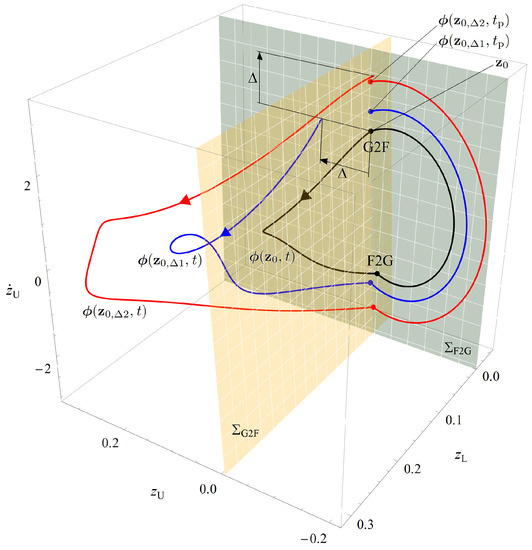
Figure 3. The switching surfaces, the periodic orbit and the perturbed trajectories. The dots indicate the intersection with switching surfaces ${\Sigma }_{\mathrm{G}2\mathrm{F}}$ and ${\Sigma }_{\mathrm{F}2\mathrm{G}}$. Note: state variable ${\dot{z}}_2$ has a jump after reaching ${\Sigma }_{\mathrm{F}2\mathrm{G}}$, which cannot be seen explicitly here.

4.2. Illustration of Periodic Solutions

This section shows the periodic solution for a case example with a certain parameter set, which is the following: $g=9.81[\mathrm{m}/\mathrm{s}]$, $m=75\left[\mathrm{kg}\right]$, $\mu =0.8\left[1\right]$, $k=\mathrm{15,000}[\mathrm{N}/\mathrm{m}]$, $d_{\mathrm{F}}=150[\mathrm{Ns}/\mathrm{m}]$, $d_{\mathrm{G}}=-80[\mathrm{Ns}/\mathrm{m}]$ and $L_0=1\left[\mathrm{m}\right]$ which is the distance of the particles with unstretched spring. The following parameters are obtained from the values above: $\alpha =\sqrt{k/m}=14.14[1/\mathrm{s}]$, $D_{\mathrm{G}}=d_{\mathrm{G}}/\left(2\alpha m\right)=-0.0377\left[1\right]$, $m_{\mathrm{U}}=60\left[\mathrm{kg}\right]$ and $m_{\mathrm{L}}=15\left[\mathrm{kg}\right]$.

Figure 3 shows a typical periodic orbit $\mathbf{\varphi }({\mathbf{z}}_0,t)$ in the $z_1$, $z_2$ and ${\dot{z}}_1$ subspace. Also, the perturbed trajectories $\mathbf{\varphi }({\mathbf{z}}_{0,\Delta 1},t)$ and $\mathbf{\varphi }({\mathbf{z}}_{0,\Delta 2},t)$ are illustrated. For the sake of better illustration of the idea of the stability analysis, the initial conditions are perturbed by a large number instead of the small number $\Delta$ (see Section 4.1.4). The perturbations of initial conditions (65) and (66) are therefore visible. The quantities $\mathbf{\varphi }({\mathbf{z}}_{0,\Delta 1},t_{\mathrm{p}})-{\mathbf{z}}_0$ and $\mathbf{\varphi }({\mathbf{z}}_{0,\Delta 2},t_{\mathrm{p}})-{\mathbf{z}}_0$, from which the Jacobian matrix (67) is constructed, are also visible here.

The stability is determined in two alternative ways, as we explained in Section 3.5. The monodromy matrix $\tilde{\mathsf{\Phi }}$ (see 36) was calculated by means of the variational Equations (34) and (35). Additionally, the approximation of the Floquet multipliers was calculated with the help of the Jacobian $\mathbf{M}$ (see (32) and (67)). $\mathbf{M}$ and the fundamental solution matrix $\tilde{\mathsf{\Phi }}$ at the end of the period and their eigenvalues are

$$\mathbf{M}=\left[\begin{array}{cc}0.0175& 0.0024\\ 3.28& 0.453\end{array}\right],$$

(68)

$$\tilde{\mathsf{\Phi }}\left(t_{\mathrm{G}2\mathrm{F}}\right)=\left[\begin{array}{cccc}-0.729& -0.134& -0.248& -0.0634\\ 0& 0& 0& 0\\ 11.41& 4.19& 3.18& 0.803\\ -11.45& -2.27& -3.84& -0.980\end{array}\right],$$

(69)

$$\mathit{\mu }=\left[\begin{array}{cc}0.4714,& 0\end{array}\right],$$

(70)

$$\mathit{\nu }=\left[\begin{array}{cccc}1,& 0.4714,& 0,& 0\end{array}\right]$$

(71)

in the specified parameter set. The system is stable with the current parameter set, since the largest relevant eigenvalue is ${\mu }_1={\nu }_2=0.4714<1$.

To illustrate the discontinuities in the system, the sections of the phase-space are shown in Figure 4 separately for the coordinates $z_{\mathrm{U}}$ and $z_{\mathrm{L}}$. The jump defined by the function, which appears in (12) and (26), is illustrated in the right panel. The switching surfaces ${\Sigma }_{\mathrm{F}2\mathrm{G}}$ defined by (11) and ${\Sigma }_{\mathrm{G}2\mathrm{F}}$ defined by (13) are visible in the right and left panel of Figure 4 respectively.

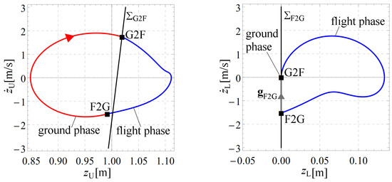
Figure 4. Phase portraits for particle $m_{\mathrm{U}}$ (left panel) and $m_{\mathrm{L}}$ (right panel). The switching surfaces are indicated by black lines. Here, the jump of state variable ${\dot{z}}_{\mathrm{L}}$ can be seen. The trajectory of particle $m_{\mathrm{L}}$ in the ground phase is represented by point G2F.

Figure 5 shows the time history of the mechanical energy. The constrained motion space kinetic energy $T_{\mathrm{c}}$ and the admissible motion space kinetic energy $T_{\mathrm{a}}$ (CMSKE and AMSKE) can clearly be seen here. The kinetic energy of the lower mass block is constant zero during the entire ground phase because of the inelastic ground-foot collision. Although CMSKE is absorbed in each F2G transition, the energy level at the end of the period reaches the value that corresponds to the beginning of the period. The extra energy is pumped to the system by the negative damper during the ground phase.

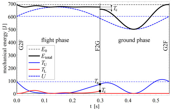
Figure 5. Time history of kinetic and potential energy. The absorbed amount of kinetic energy (CMSKE) and the remaining part are indicated by $T_{\mathrm{c}}$ and $T_{\mathrm{a}}$ respectively. The total mechanical energy $E_{\mathrm{total}}$ converges to the nominal level $E_0$ in each jump.

The time histories for all state variables were in correspondence in the semi-analytical and in the numerical calculation.

4.3. Overview of Effect of Parameters

To gain an overview of the effect of physical and control parameters, the portion $\mu$ of the masses and the negative damping value $D_{\mathrm{G}}$ were varied by means of a numerical continuation. Parameter $\mu$ was set to the discrete values 0.8 and 0.95. For each $\mu$ values, $D_{\mathrm{G}}$ was continuously decreased from zero until the periodic orbits disappear. Compared to [24], it is a new result about the hopping model that the unstable periodic orbits were found, not only the stable ones.

Plotting the flight phase time period $t_{\mathrm{F}}$, the ground phase time period $t_{\mathrm{G}}$ and the entire time period $t_{\mathrm{p}}$ in Figure 6 provides a general look of the dynamic behavior of the system. Above $D_{\mathrm{G}}=0$ values there is no periodic solution, since both dampers continuously absorb energy, which leads to static equilibrium. In the $D_{\mathrm{G}}=0$ case, the time period $t_{\mathrm{G}}$ of the ground phase is exactly equal to the time period $t_{\mathrm{p}0}=2\pi \sqrt{m_{\mathrm{u}}/k}$ of the 1 DoF oscillatory system composed by spring k, damper $d_{\mathrm{G}}=0$ and mass $m_{\mathrm{u}}$. For $D_{\mathrm{G}}>0$ cases, the ground phase time period $t_{\mathrm{G}}$ becomes infinity, since the lower mass block never takes off from the ground. When increasing $D_{\mathrm{G}}$ in the negative direction, one or more stable periodic orbits can be found with different time periods. Finally, the flight phase time period goes to infinity. This is the point, when the Floquet multipliers shown in Figure 7 would cross the 1 value.

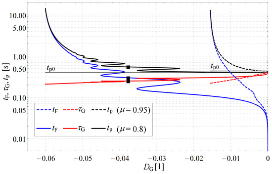
Figure 6. The flight phase time period, the ground phase time period and the entire time period.

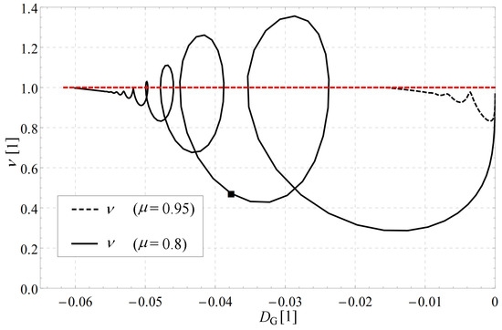
Figure 7. Relevant eigenvalue with different parameters.

Figure 8 shows the apex height of the $z_{\mathrm{U}}$ and $z_{\mathrm{L}}$ trajectories. The hopping height is in close relation with the flight phase time duration $t_{\mathrm{F}}$, which can be seen by comparing the graphs in Figure 6 and Figure 8. In the extreme values of the ground phase damping parameter $D_{\mathrm{G}}$, the hopping height is such small or such large that are practically irrelevant. In the middle range, the hopping height is realistic for humans, according to [6,7].

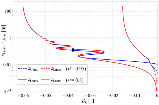
Figure 8. Apex height of the trajectory with different parameters.

The ratio of the CMSKE and the AMSKE (absorbed and preserved amount of kinetic energy) to the total kinetic energy T are plotted in Figure 9. One can notice that the AMSKE value denoted by $T_{\mathrm{a}}$ converges to the $\mu$ value as $D_{\mathrm{G}}$ decreases. We can conclude that it is possible to find optimal parameter set when the ratio of CMSKE is the smallest. Since CMSKE in in relation to the impact intensity and is indirectly in relation to the risk of injuries, this may be a cost function in running and walking systems.

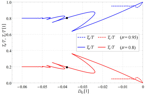
Figure 9. Ratio of constrained and admissible motion space kinetic energy with different parameters.

The Floquet multiplier, which determines the stability of the periodic orbits, is plotted in Figure 7. The results show that the stability highly depends on both physical ($\mu$) and control ($D_{\mathrm{G}}$) parameters. At $D_{\mathrm{G}}=0$ the Floquet multiplier is exactly 1, since in that case a 1 DoF undamped oscillation occurs with constant amplitude. By decreasing the numerical value of $D_{\mathrm{G}}$, the Floquet multiplier reaches 1 and the time period of the orbit becomes infinitely long (see Figure 6). Comparing Figure 7 and Figure 8, one can notice that stable periodic orbits are separated from each other by unstable periodic orbits. The combination of apex height, stability and impact intensity may be applied as a combined cost function in certain applications in the field of legged robotic systems.

Our dynamic analysis methodology presented in Section 3 makes possible to obtain similar continuation result for complex multibody models with high DoF and geometric constraints.

5. Conclusions and Future Work

We further developed a minimally complex model of hopping resulting in a constrained model, on which our dynamic analysis methodology was demonstrated. In general, the constrained models are described by a non-minimum set of coordinates and the equations of motion are augmented with geometric constraint equations. This modeling approach, which is typical in multibody dynamics, allows us to build high DoF models effectively. The dynamic analysis methodology of piecewise-smooth systems was generalized for such constrained multibody systems in this study.

The presented dynamic analysis methodology focuses on the stability investigation of periodic orbits of hopping and running models that consider control issues, geometric non-linearities, inelastic ground-foot collision and energetic costs in relation to the collisions. The controller in our models generates the motion pattern without any prescribed kinematics. Instead, such sets of the physical and the control parameters are identified that assure stable periodic motion.

The limitation of the model and the presented dynamic analysis is that the motion is strictly divided into two phases: flight and ground. Furthermore, we consider only single support in the ground phase. The dynamic analysis methodology will be further developed to handle multiple ground support.

We demonstrated our dynamic analysis method on a vertically hopping constrained model. The results were compared with semi-analytically obtained reference results of the corresponding unconstrained model: the periodic orbits, the parameter set that guarantees stable operation, the Floquet multipliers and energy loss induced by the ground collision were in total correspondence.

In future work, we will apply the present dynamic analysis for higher DoF models of hopping and running. We will particularly focus on ground-foot collision, since foot collision is the main source of injuries when walking and running. Furthermore, a considerable amount of energy- demand of locomotion is related to ground-foot collision.

References

- Alciatore, D.; Abraham, L.; Barr, R. Matrix Solution of Digitized Planar Human Body Dynamics for Biomechanics Laboratory Instruction. Available online: http://www.engr.colostate.edu/~dga/dga/papers/bio_matrix.pdf (accessed on 13 November 2018).
- Jungers, W.L. Barefoot running strikes back. Nat. Biomech. 2010, 463, 433–434. [Google Scholar] [CrossRef] [PubMed]
- Mombaur, K.; Olivier, A.H.; Crétual, A. Forward and Inverse Optimal Control of Bipedal Running. In Modeling, Simulation and Optimization of Bipedal Walking; Mombaur, K., Berns, K., Eds.; Springer: Berlin/Heidelberg, Germany, 2013; pp. 165–179. [Google Scholar]
- Souza, R.B. An Evidence-Based Videotaped Running Biomechanics Analysis. Phys. Med. Rehabil. Clin. N. Am. 2016, 27, 217–236. [Google Scholar] [CrossRef] [PubMed]
- Ćesić, J.; Joukov, V.; Petrovic, I.; Kulić, D. Full Body Human Motion Estimation on Lie Groups Using 3D Marker Position Measurements. In Proceedings of the IEEE-RAS International Conference on Humanoid Robotics, Cancun, Mexico, 15–17 November 2016; p. 8. [Google Scholar]
- Vanezis, A.; Lees, A. A biomechanical analysis of good and poor performers of the vertical jump. Ergonomics 2005, 48, 1594–1603. [Google Scholar] [CrossRef] [PubMed]
- Kamandulis, S.; Venckunas, T.; Snieckus, A.; Nickus, E.; Stanislovaitiene, J.; Skurvydas, A. Changes of vertical jump height in response to acute and repetitive fatiguing conditions. Sci. Sports 2016, 31, 163–171. [Google Scholar] [CrossRef]
- Lieberman, D.E.; Venkadesan, M.; Werbel, W.A.; Daoud, A.I.; D’Andrea, S.; Davis, I.S.; Mang’Eni, R.O.; Pitsiladis, Y. Foot strike patterns and collision forces in habitually barefoot versus shod runners. Nat. Biomech. 2010, 463, 531–535. [Google Scholar] [CrossRef] [PubMed]
- Zelei, A.; Bencsik, L.; Kovács, L.L.; Stépán, G. Energy efficient walking and running-impact dynamics based on varying geometric constraints. In Proceedings of the 12th Conference on Dynamical Systems Theory and Applications, Lodz, Poland, 2–5 December 2013; pp. 259–270. [Google Scholar]
- Seyfarth, A.; Günther, M.; Blickhan, R. Stable operation of an elastic three-segment leg. Biol. Cybern. 2001, 84, 365–382. [Google Scholar] [CrossRef] [PubMed]
- Holmes, P.; Full, R.J.; Koditschek, D.E.; Guckenheimer, J. The Dynamics of Legged Locomotion: Models, Analyses, and Challenges. SIAM Rev. 2006, 48, 207–304. [Google Scholar] [CrossRef]
- Rummel, J.; Seyfarth, A. Stable Running with Segmented Legs. Int. J. Robot. Res. 2008, 27, 919–934. [Google Scholar] [CrossRef]
- Clever, D.; Hu, Y.; Mombaur, K. Humanoid gait generation in complex environments based on template models and optimality principles learned from human beings. Int. J. Robot. Res. 2018. [Google Scholar] [CrossRef]
- DeHart, B.J.; Gorbet, R.; Kulić, D. Spherical Foot Placement Estimator for Humanoid Balance Control and Recovery. In Proceedings of the International Conference on Robotics and Automation, Brisbane, Australia, 21–25 May 2018; p. 8. [Google Scholar]
- Stépán, G. Delay effects in the human sensory system during balancing. Trans. R. Soc. A 2009, 367, 1195–1212. [Google Scholar] [CrossRef] [PubMed]
- Insperger, T.; Milton, J.; Stépán, G. Acceleration feedback improves balancing against reflex delay. J. R. Soc. Interface 2013, 10, 20120763. [Google Scholar] [CrossRef] [PubMed]
- Milton, J.; Insperger, T.; Cook, W.; Harris, D.M.; Stepan, G. Microchaos in human postural balance: Sensory dead zones and sampled time-delayed feedback. Phys. Rev. E 2018, 98. [Google Scholar] [CrossRef] [PubMed]
- Beer, R.D. Beyond control: The dynamics of brain-body-environment interaction in motor systems. Adv. Exp. Med. Biol. 2009, 629, 7–24. [Google Scholar] [CrossRef] [PubMed]
- Fekete, L.; Krauskopf, B.; Zelei, A. Three-segmented hopping leg for the analysis of human running locomotion. In Proceedings of the 9th European Nonlinear Dynamics Conference (ENOC 2017), Budapest, Hungary, 25–30 June 2017; pp. 1–2. [Google Scholar]
- Zelei, A.; Insperger, T. Reduction of ground-foot impact intensity of a hopping leg model on slopes. In Proceedings of the 5th Joint International Conference on Multibody System Dynamics–IMSD 2018, Lisboa, Portuga, 24–28 June 2018. [Google Scholar]
- Piiroinen, P.T.; Dankowicz, H.J. Low-Cost Control of Repetitive Gait in Passive Bipedal Walkers. Int. J. Bifurca. Chaos 2005, 15, 1959–1973. [Google Scholar] [CrossRef]
- Kövecses, J.; Kovács, L.L. Foot impact in different modes of running: Mechanisms and energy transfer. Procedia IUTAM 2011, 2, 101–108. [Google Scholar] [CrossRef]
- Novacheck, T.F. The biomechanics of running. Gait Posture 1998, 7, 77–95. [Google Scholar] [CrossRef]
- Zelei, A.; Insperger, T. Simplest mechanical model of stable hopping with inelastic ground-foot impact. In Proceedings of the 12th IFAC Symposium on Robot Control—SYROCO 2018, Budapest, Hungary, 27–30 August 2018; p. 6. [Google Scholar]
- De Jalón, J.; Bayo, E. Kinematic and Dynamic Simulation of Multibody Systems: The Real-Time Challenge; Springer: Berlin, Germany, 1994. [Google Scholar]
- Featherstone, R.; Orin, D. Robot dynamics: Equations and algorithms. In Proceedings of the ICRA 2000, IEEE International Conference on Robotics and Automation, San Francisco, CA, USA, 24–28 April 2000; pp. 826–834. [Google Scholar] [CrossRef]
- De Jalón, J.G. Twenty-five years of natural coordinates. Multibody Syst. Dyn. 2007, 18, 15–33. [Google Scholar] [CrossRef]
- Johnson, A.M.; Koditschek, D.E. Legged Self-Manipulation. IEEE Access 2013, 1, 310–334. [Google Scholar] [CrossRef]
- Peters, S.; Hsu, J. Comparison of Rigid Body Dynamic Simulators for Robotic Simulation in Gazebo. 2014. Available online: https://www.osrfoundation.org/wordpress2/wp-content/uploads/2015/04/roscon2014_scpeters.pdf (accessed on 13 November 2018).
- Johnson, A.M.; Burden, S.A.; Koditschek, D.E. A hybrid systems model for simple manipulation and self-manipulation systems. Int. J. Robot. Res. 2016, 35, 1354–1392. [Google Scholar] [CrossRef]
- Leine, R.I. Bifurcations in Discontinuous Mechanical Systems of Fillipov Type. Ph.D. Thesis, Technische Universiteit Eindhoven, Eindhoven, The Netherlands, 2000. [Google Scholar]
- Dankowicz, H.J.; Piiroinen, P.T. Exploiting discontinuities for stabilization of recurrent motions. Dyn. Syst. 2002, 17, 317–342. [Google Scholar] [CrossRef]
- Burden, S.A.; Sastry, S.S.; Koditschek, D.E.; Revzen, S. Event-Selected Vector Field Discontinuities Yield Piecewise-Differentiable Flows. SIAM J. Appl. Dyn. Syst. 2016, 15, 1227–1267. [Google Scholar] [CrossRef]
- Kövecses, J.; Piedoboeuf, J.C.; Lange, C. Dynamic Modeling and Simulation of Constrained Robotic Systems. IEEE/ASME Trans. Mechatron. 2003, 2, 165–177. [Google Scholar] [CrossRef]
- Westervelt, E.R.; Grizzle, J.W.; Chevallereau, C.; Choi, J.H.; Morris, B. Feedback Control of Dynamic Bipedal Robot Locomotion; CRC Press: Boca Raton, FL, USA, 2007. [Google Scholar]
- Hiskens, I.A.; Pai, M.A. Trajectory sensitivity analysis of hybrid systems. IEEE Trans. Circuits Syst. I Fundam. Theory Appl. 2000, 47, 204–220. [Google Scholar] [CrossRef]
- Zelei, A.; Krauskopf, B.; Insperger, T. Control optimization for a three-segmented hopping leg model of human locomotion. In Proceedings of the DSTA 2017—Vibration, Control and Stability of Dynamical Systems, Lodz, Poland, 11–14 December 2017; pp. 599–610. [Google Scholar]
- Koditschek, D.E.; Buehler, M. Analysis of a Simplified Hopping Robot. Int. J. Robot. Res. 1991, 10, 587–605. [Google Scholar] [CrossRef]
- Leine, R.I.; van Campen, D.H. Discontinuous bifurcations of periodic solutions. Math. Comput. Model. 2002, 36, 259–273. [Google Scholar] [CrossRef]
- Blajer, W.; Dziewiecki, K.; Mazur, Z. An improved inverse dynamics formulation for estimation of external and internal loads during human sagittal plane movements. Comput. Methods Biomech. Biomed. Eng. 2015, 18, 362–375. [Google Scholar] [CrossRef] [PubMed]
- Font-Llagunes, J.M.; Pamies-Vila, R.; Kövecses, J. Configuration-Dependent Performance Indicators for the Analysis of Foot Impact in Running Gait. Available online: http://www.cim.mcgill.ca/~font/downloads/ECCOMAS13.pdf (accessed on 13 November 2018).
- Yamakita, M.; Asano, F. Extended passive velocity field control with variable velocity fields for a kneed biped. Adv. Robot. 2001, 15, 139–168. [Google Scholar] [CrossRef]
- Kövecses, J.; Font-Llagunes, J.M. An Eigenvalue Problem for the Analysis of Variable Topology Mechanical Systems. ASME J. Comput. Nonlinear Dyn. 2009, 4, 9. [Google Scholar] [CrossRef]
- Chi, K.J.; Schmitt, D. Mechanical energy and effective foot mass during impact loading of walking and running. J. Biomech. 2005, 38, 1387–1395. [Google Scholar] [CrossRef] [PubMed]
- Dankowicz, H.; Schilder, F. Recipes for Continuation, Computational Science and Engineering; Society for Industrial and Applied Mathematics: Philadelphia, PA, USA, 2013. [Google Scholar]
- Guckenheimer, J.; Holmes, P. Nonlinear Oscillations, Dynamical Systems, and Bifurcations of Vector Fields; Springer: Berlin, Germany, 1983. [Google Scholar]
- Ewins, D. Modal Testing: Theory and Practice; John Wiley and Sons: Hoboken, NJ, USA, 1984. [Google Scholar]
- He, J.; Fu, Z.F. Modal Analysis; Elsevier: Amsterdam, The Netherlands, 2001. [Google Scholar]
© 2018 by the authors. Licensee MDPI, Basel, Switzerland. This article is an open access article distributed under the terms and conditions of the Creative Commons Attribution (CC BY) license (http://creativecommons.org/licenses/by/4.0/).