Trustworthiness in Modeling Unreinforced and Reinforced T-Joints with Finite Elements

Abstract

As required by regulations, Finite Element Analyses (FEA) can be used to investigate the behavior of joints which might be complex to design due to the presence of geometrical and material discontinuities. The static behavior of such problems is mesh dependent, thus these results must be calibrated by using laboratory tests or reference data. Once the Finite Element (FE) model is correctly setup, the same settings can be used to study joints for which no reference is available. The present work analyzes the static strength of reinforced T-joints and sheds light on the following aspects: shell elements are a valid alternative to solid modeling; the best combination of element type and mesh density for several configurations is shown; the ultimate static strength of joints can be predicted, as well as when mechanical properties are roughly introduced for some FE topologies. The increase in strength of 12 unreinforced and reinforced (with collar or doubler plate) T-joints subjected to axial brace loading is studied. The present studies are compared with the literature and practical remarks are given in the conclusion section.

1. Introduction

Joints in offshore engineering are crucial because they are key components in the design of jacket structures. The study of joints is generally performed after a pre-dimensioning of the complete jacket has been carried out. Jacket structures are investigated using simple lattice models made of beams which simulate the tubular elements of the whole structures. Such simple model is extremely convenient for global structural analysis but does not give enough detail regarding local structural failure such as fatigue cracking at joints. For this reason, several authors in the past and recent years investigated the problem of static and dynamic strength of offshore extensively [1,2,3,4,5,6,7,8,9,10,11,12,13,14,15,16,17]. Among these, Moffat et al. [1] investigated the effect of the chord length and the applied boundary conditions on the static strength of tubular T-joints. Ring stiffened DT-joints (cross shaped) have been studied by Marcus et al. [3]; the dynamic performance of collar plate reinforced joints was studied by Qu et al. [10]. Numerical and experimental studies on the ultimate strength of KT-joints (K shaped) were presented by Li et al. [15].

On the other hand, in the recent studies some researchers have investigated in detail the concertation of the stress and its distribution in critical areas [18,19,20,21,22,23], where Lostsberg [18], Osawa et al. [19] and Lotfollahi-Yagin et al. [20] have focused on the stress hot spots in tubular joints, whereas, Cheng et al. [21] investigated how the concertation of the stress affect the fatigue.

In addition to the aforementioned researches, other studies that involved joints should be mentioned [24,25,26,27,28,29,30,31,32,33,34,35,36,37,38,39,40,41,42,43,44,45,46], such as the work by Xia et al. [24] regarding the hysteretic behavior of stiffened T-joints. Furthermore, Dong et al. [28] presented long-term fatigue analysis of multi-planar tubular joints. Finally, experimental tests were performed on joints using white light speckle method by Liu [32]. Numerical implementation and coupling of finite elements of different topology in the study of joints were proposed by Pey et al. [33], and a good review on finite and boundary element methods was given by Mackerle [34,35]. Regarding the topic of composite structures, the work by Chowdhury et al. [41] and Shen et al. [42] should be cited for their application to practical engineering practices for the static and fatigue strength of joints. Finally, the parametric study on composite joints by Liu et al. [46] is mentioned for their thorough description of this particular problem.

The present work investigates tubular joints made of steel Circular Hollow Sections (CHSs) that are the main structural components of steel off-shore structures such as jackets, compliant towers, jack-ups, etc. In these kinds of structures, the CHSs members are joined in a point, forming a tubular simple joint by welding the profiled ends of the secondary members, the braces, onto the circumference of the main member, the chord.

Due to their crucial rule, some guidelines and methods have been introduced, to guarantee the needed serviceability and to understand the strength behavior of these type of element, the most used are: American Petroleum Institute (API) [47], International Organization for Standardization (ISO) [48], American Bureau of Shipping (ABS) [49], and Eurocode3 (EC3) [50].

Several types of reinforcement are available nowadays in order to enhance the strength of tubular joints. One typology that can be found often in off-shore is schematically shown in the sections depicted in Figure 1, where the collar plate (a) consists in flat surface around the brace-chord intersection, whereas the doubler plate (b) is a surface in between the two elements. These two methods are widely used since they can be an important improvement either for rehabilitation purposes in old structures or for new structures.

Thus, for a better understanding of the static strength of joints with the introduction of the two types of reinforcement, 12 T-Joint specimens subjected to axial brace load (6 in compression and 6 in tension) have been studied, with different geometric and material parameters. T-joints have been selected in this investigation even though several types of joints can be formed in lattice structures such as Y, K, and X joints or their combinations. Based on this study, conclusions can be obtained in assessing the reinforcing efficiency.

The aforementioned guidelines [47,48,49,50] suggest using FE models whenever new configuration of joint are treated, but the sharp geometric discontinuities (wherein stress concentrations occur) in the tubular joints lead to a mesh dependence for the results and so such FE models need to be calibrated by considering reference data such as laboratory tests. In the present paper, the works [4,5] have been considered as a reference.

The reference paper [5] considers a 3-D solid FE model, on the contrary the present research simplifies the problem by modeling the joints with less degrees of freedom and a much simpler geometric description. Shell elements are used in this research because of their simplicity and the lower cost in terms of computational time with respect to solid elements. Moreover, the geometry of FE models made of solid elements is more difficult to generate and assemble with respect to 2-D shell elements. In the reference 3-D simulations [5] the authors decided to deploy solid elements instead of 2-D elements, mainly because: the contact algorithm will only identify contact between two members if the shell elements (which represent the mid-surfaces of each member) touch each other, thereby incorrectly allowing penetration of one member into the other, in addition to preventing the uncertainty in modeling the welded area of the brace-chord intersection. Therefore, succeeding in solving the aforementioned limits, as will be showed in the following sections, shell elements can be used instead of solid elements as in the present research.

The present work considers the commercial finite element ABAQUS package, since it offers an attractive alternative to generate reliable data, provided that the accuracy of the FE model is firstly verified against test evidence. In particular, ABAQUS 6.14 will be used for all the simulations.

2. Previous Researches

The aim of the work, as has been already aforementioned, is to improve the understanding of the static behavior of plate reinforced joints, by building an FE model with shell elements. This is generally required from the regulations when new joint configurations are studied, but since stress concentrations computed by FE are mesh dependent, they need to be calibrated with the help of laboratory tests [4].

The reference papers present an experimental investigation and a numerical simulation. The numerical simulation has been considered here to have the possibility of discussing the improvement that have been obtained by the use of a different element topology. In this section, relevant information will be summarized. However, for an exhaustive description of the tests, the reader is invited to the articles [4,5].

2.1. Experimental Investigations

Laboratory tests are one useful way to calibrate numerical simulations. The basic configuration and the T-joint geometries are illustrated in Figure 1. The experimental program consists of 12 tests, of unreinforced and reinforced with collar or doubler plates, as depicted in Figure 1. Joints have been tested under both compression and tension loading. The geometric data indicated in Figure 1 are listed in

Table 1. Geometrical details of the twelve T-joint specimens.

	Type	${\mathit{d}}_0$	${\mathit{d}}_1$	${\mathit{t}}_0$	${\mathit{t}}_1$	${\mathit{t}}_{\mathit{d}}$	Brace Loading
$EX-01$	Unreinforced	409.5	221.9	8.1	6.8	-	Compression
$EX-02$	Unreinforced	409.5	221.9	8.1	6.8	-	Tension
$EX-03$	Collar	409.5	221.9	8.1	6.8	6.4	Compression
$EX-04$	Collar	409.5	221.9	8.5	6.8	6.4	Tension
$EX-05$	Collar	409.5	221.9	12.8	8.4	8.3	Compression
$EX-06$	Collar	409.5	221.9	12.8	8.4	8.3	Tension
$EX-07$	Doubler	409.5	221.9	8.5	6.8	6.6	Compression
$EX-08$	Doubler	409.5	221.9	8.2	6.5	6.4	Tension
$EX-09$	Unreinforced	409.5	114.7	8.5	5.9	-	Compression
$EX-10$	Unreinforced	409.5	114.7	8.5	5.9	-	Tension
$EX-11$	Doubler	409.5	114.7	8.5	5.9	6.6	Compression
$EX-12$	Doubler	409.5	114.7	8.5	5.9	6.6	Tension

, except for the joint lengths that are constant for all twelve specimens, respectively: $l_0=2840$ mm, $l_1=1100$ mm, and $l_d=l_c=305$ mm.

The materials used in each test are fabricated from carbon steel pipe, using the guidelines given from the API 5L Gr. B/ASTM A106-94A; while the welding procedure follows AWS D1.1.

Table 2. Material properties and yield stresses of the twelve T-joint specimens.

	$\begin{array}{c}{\mathit{f}}_{\mathit{y},0}\\ [\mathit{N}/\mathit{m}{\mathit{m}}^2]\end{array}$	$\begin{array}{c}{\mathit{f}}_{\mathit{y},1}\\ [\mathit{N}/\mathit{m}{\mathit{m}}^2]\end{array}$	$\begin{array}{c}{\mathit{f}}_{\mathit{y},\mathbf{d}}\\ [\mathit{N}/\mathit{m}{\mathit{m}}^2]\end{array}$
$EX-01$	285	300	-
$EX-02$	285	300	-
$EX-03$	285	300	461
$EX-04$	276	300	461
$EX-05$	276	275	464
$EX-06$	276	275	464
$EX-07$	276	300	461
$EX-08$	312	284	461
$EX-09$	276	312	-
$EX-10$	276	312	-
$EX-11$	276	312	461
$EX-12$	276	312	461

indicates the measured yield stress for each steel component of the chord $f_{y,0}$, brace $f_{y,1}$, and reinforcement $f_{y,d}$.

Each specimen is pin-supported at the chord ends to minimize the possibility of axial load, and the brace is bolted at the top. The load is applied through a displacement-controlled actuator that has a rated compression capacity of 2000 kN, a tension capacity of 1200 kN, and range of displacement of ±200 mm. In all tests, the load is applied at initial stage at rate of 0.3 mm/min for the linear part and increased up to 1.2 mm/min through the Instron 8800 controller [4].

2.2. Numerical Simulations

The present section illustrates the details of the numerical simulations performed with 3-D solid elements in the reference [5]. Strength and weaknesses of all the modeling details provided are listed below.

The analysis considers the dimensions of the tubular members reported in Table 1, whereas for the materials proprieties Table 2 has been considered. Major aspects of the reference FE strategy adopted for the T-joints test, such as element type, mesh density, and contact interaction, are described below.

The T-joint specimen is simply supported with symmetric brace axial load [5], therefore the model has been simplified by considering a quarter of the whole model; and solid elements were selected to model the tubular joints, obviously these elements account for the joint dimensions in all three directions. Alternatively, mesh size is composed in such a way to be relatively smaller where the stress gradient is more critical, therefore the density of the mesh decreases from the vicinity of the intersection to the end of the brace or chord.

In the reference [5], the authors stated that: “Weld geometry was modeled using a ring of shell elements along the brace-chord” and that: “the penetration weld between the brace and the doubler plate is modeled in accordance with the measured dimensions obtained from the T-joint specimens”. However, the graphical representation, presented in the papers [4,5], shows solid elements also for the welded area, instead of the mentioned shell elements. Therefore, a detailed size of the weld is not given in [4] or [5].

Since in this case the plate reinforced joints are loaded by an axial force/displacement, contact shall occur between bottom surface of the reinforcement and the external surface of the chord. Thus, contact plays a main rule as transferring mechanism from the secondary element (brace) to the primary one (chord), and this is a source of nonlinearity in the FE analysis. Due to the fact that both reinforcement and chord walls are deformable bodies, a deformable-deformable contact interaction is defined using a “master-slave” algorithm in the numerical analysis, with no friction between the members is assumed.

According to the experimental investigations, the axial load is applied using the displacement control method by prescribing the vertical displacement of the nodes at the brace tip.

The true stress-strain relationship enforced in these simulations is related to the yielding point of each material, as given in Table 2 , and can be represented by a bilinear relationship. No further hardening in the true stress-true strain behavior is assumed after the peak load in the engineering stress-strain curve, i.e., the true stress-true strain curve is assumed to remain horizontal beyond this point as for elastic-perfectly plastic model, as shown in Figure 2a. Contrastingly, the welds are assumed to have the same material properties as the base metal.

The use of this simplification in the true stress-strain relationship is commonly used in the design of structures because allows the designer to stay in the safety size due to the fact that no hardening is considered. This approximation, though, can lead to a result slightly different from the real behavior. For this, in Section 6, in addition to the elastic-perfectly plastic model, a model where the hardening is taken into account, as in Figure 2b, will also be considered.

2.3. Comparison Setup

More detailed information about the results of the two investigations will be given in the next section while showing the results of the work made during this research. However, in this section the main point of data collecting and how the results have been shown by the authors of [4,5] will be given. In general, the results of the two papers can be summarized in just one, since they are two parts of the same study. The results given by the references are given in terms of load-ovalization curves and deformed shapes.

The load-ovalization curves are presented, where the ovalization indicates the deformation of the chord cross section at the center of the T-joint, which is calculated by subtracting the height of point fixed simultaneously at the bottom of the chord and at the center of the joint, ${\delta }_B$, from the average value of four fixed points (in the one quarter FE model of course will be only two) on the brace near the intersection with the chord, ${\delta }_A$. These points are obtained by the transducer reading in case of experimental investigation, whereas for the FE model by using RP (Reference Point) as shown in Figure 1. The ultimate load for each test is identified simply by selecting the peak of each curve, and these values are listed in

Table 3. Ultimate load obtained in the numerical simulation [5].

	$\begin{array}{c}{\mathit{F}}_{\mathbf{u},\mathbf{t}\mathbf{e}\mathbf{s}\mathbf{t}}\\ [\mathbf{k}\mathit{N}]\end{array}$	$\begin{array}{c}{\mathit{F}}_{\mathbf{u},\mathbf{n}\mathbf{u}\mathbf{m}}\\ [\mathbf{k}\mathit{N}]\end{array}$	${\mathit{F}}_{\mathbf{u},\mathbf{n}\mathbf{u}\mathbf{m}}/{\mathit{F}}_{\mathbf{u},\mathbf{t}\mathbf{e}\mathbf{s}\mathbf{t}}$
$EX-01$	305.1	310.9	1.02
$EX-02$	543.2	557.8	1.03
$EX-03$	425.6	431.4	1.01
$EX-04$	609.2	648.9	1.07
$EX-05$	780.0	798.5	1.02
$EX-06$	1065.3	1069.3	1.00
$EX-07$	415.8	446.4	1.07
$EX-08$	708.0	712.2	1.01
$EX-09$	200.1	193.0	0.96
$EX-10$	407.8	393.7	0.97
$EX-11$	305.0	309.3	1.01
$EX-12$	520.0	506.2	0.97

, where $F_{u,test}$ is for the experimental investigations [4] while $F_{u,num}$ for the numerical simulations [5]. At the same time, the two phases of the joint behavior, such as the linear phase and the plastic one, can be deducted.

The experimental [4] and numerical [5] results are not only evaluated in terms of load-ovalization curves but also by comparison of deformed sliced “rings”, taken at the center of the T-joints after the tests and numerical analyses were completed. Then at the end of the tests, for some of the specimens, sections or “rings” were obtained for the joint elements, chord and brace.

In conclusion, all the results obtained from these two papers will be used in the fundamental step of calibration of the FE model of the present work. In the following section the results of the present FE simulations will be compared to the ones of the previous studies and comments and highlights will be provided.

3. Present Modeling

Commercial finite element packages offer an attractive and cheaper alternative to the laboratory experiments, but at the same time they require the use of sophisticated hardware, and also need the help of other software to post-processing the results. Hence, different software have been used, such as Abaqus/CAE 6.14-1 [51], Matlab R2017a, and AutoCAD 2017. The hardware used is the Intel(R) Core(TM) i7-4700MQ CPU @ 2.40GHz 2.40 GHz with 12GB of RAM.

This section addresses various aspects of all the steps that have been performed to study and simulate the state of T-joints subjected to the axial force. The cheaper shell elements have been used in this work, whereas the numerical simulation made in [5] considered solid elements.

The dimensions of the tubular members and reinforcement plates assumed in this research are in accordance with the measured dimensions of the test specimen of the papers as sketched in Figure 1, for which the values are reported in Table 1. In contrast, Table 2 summarizes the measured yield stress for each chord $f_{y,0}$, brace $f_{y,1}$, and reinforcement $f_{y,d}$.

Although the type of element material is specified in the reference papers [4,5] as carbon steel, the characteristics of this typology of material are not unique, especially concerning Young’s Modulus ($E$) and Poisson ratio ($\nu$), where $E$ ranges from 203 to 210 GPa whereas $\nu$ ranges from 0.25 to 0.3. With the help of preliminary simulations, the more fitting values of these have been demonstrated to be $E=210\mathrm{GPa}$ and $\nu =0.3$. These values were obtained by comparing the normalized load $R$, defined as $R=F_{u,test}/f_{y,0}\cdot t_0^2$ of the EX-01, where $t_0^{}$ is the chord thickness, with the one given by the experimental investigations, as reported in

Table 4. Values of E and ν of preliminary simulations [17].

Specimen	Experimental Investigation	Preliminary Simulation 1 $\mathit{E}=$203 ν = 0.25	Preliminary Simulation 2 $\mathit{E}=$210 ν = 0.25	Preliminary Simulation 3 $\mathit{E}=$210 ν = 0.30
$f_{y,0}{[\mathrm{N}/\mathrm{mm}}^2]$	285	285	285	285
$t_0\left[\mathrm{mm}\right]$	8.1	8.1	8.1	8.1
$R=F_{u,test}/f_{y,0}\cdot t_0^2$	16.32	13.95	14.09	14.11

.

AutoCAD 3D was selected to draw the T-joint tubular elements. Although ABAQUS gives the possibility to directly represents different geometries, AutoCAD is a more suitable software for this kind of parametric research since it gives the possibility to easily modify and change elements on it. Afterwards, only a quarter of the joint has been imported in the FE packages, this idealization does not make any differences in the results and reduces the total computational effort.

Starting from the first adjustments of the simulations, the three cases are discussed below: unreinforced, collar plate reinforcement, and doubler plate reinforcement.

Three native parts have been created for the reinforced cases (chord, brace, and reinforcement plate), and only two for the unreinforced case because no reinforcement is present. Some internal parts have been introduced in the part module, with their respective edges. In other words, due to the fact that the joint is made of several parts and contact must be implemented in order to connect the different parts together, construction edges (from CAD) are kept in the FE model also in order to simplify the following step.

Once all the parts are created (in their own coordinate system), they should be assembled in the Abaqus Assembly module [51] that is used to create instances of the parts and to position the instances relative to each other in a global coordinate system. The instances made for all the three cases are one for each part. Then for the unreinforced case, two instances have been generated, one for the chord and the other for the brace; whereas for the reinforced cases a third instance that represents the reinforcement is present.

The displacement induced by the controlled actuator in the experimental investigation [4] is at an initial stroke rate of 0.3 mm/min, and then progressively increased up to 1.2 mm/min through the Instron 8800 controller. During the simulations in the present study, two types of step sequences are analyzed: the first automatic step sequence, and the second fixed step sequence, i.e., varying the load range during the simulations.

The automatic step sequence has the same step range for the whole simulation. While the fixed ones in order to reproduce the experimental investigation have two different ranges, in particular the second step starts at the starting point of the material plasticization which has been identified during the automatic step sequence.

The restraints that have been adopted for the FE model are in accordance with the experimental investigation; where the specimen is pin-supported at the chord ends and the brace end is bolted to the Instron actuator mounted on top of the brace, where the load is obtained as reaction force from the boundary condition at the brace tip. Since one-quarter of the whole specimen has been modeled, along with symmetry planes, peculiar boundary conditions have been considered as XSYMM (along the x-axis) and ZSYMM (along the z-axis) [51].

Material properties of the elements are modeled in accordance to the experimental investigation as listed in Table 2, whereas the Young’s modulus and Poisson ratio are taken from the preliminary simulations already described Table 4. The true stress-strain curve that has been assumed by var der Vegte et al. [5] in his numerical simulations is represented by a multilinear relationship and subsequently converted into a true stress-true strain relationship, and no further hardening in the true stress-true strain behavior is assumed after the peak load, i.e., the curve is assumed horizontal beyond this point.

Since no more detailed information is given about the true strain-stress curve, in this study, the elastic-perfectly plastic model is assumed to fit these characteristics as shown in Figure 2a. Due to the lack in the reference paper [5] for what concerns the latter relationship, in this research some hardening will be considered during the simulations, by introducing a hardening of 10% for all the materials, as depicted in Figure 2b, to verify the reliability of the elastic-perfectly plastic model.

Currently, the following types of constraints have been used in the simulations, the multi-point constraints (MPC) [51], which allows the restriction imposed by the boundary conditions (BCs) along the whole circumference, and the TIE [51], which instead has been used to connect the edges of the elements to simulate the welded connections. However, since the brace is directly welded to the chord in the unreinforced cases, no separation will occur between the two elements and the two parts have been merged (i.e., combine two elements in one instance [51]) into a single one.

During the development of the contact between the chord and the reinforcement made for the reinforced T-joints, contact mechanical properties are imposed by fixing the relevant points, such as tangential and normal behavior in the contact interaction propriety. The tangential behavior was imposed as “Frictionless”, while the normal behavior as “Hard” contact. The contact properties are also imposed to “Allow separation after contact” since, in the case of the reinforced plate, separation between the plate and the chord that are linked, by the “tie” constraints, might occur. After the contact property is defined, surface-to-surface contact interaction is set up. Here the sliding is finite, and no adjustments are required since the two surfaces lie in the same plane. A further important feature is “Contact controls” option, which helps the convergence of the simulation without considering the penetration of one member into the other, as after solved using the Top/Bottom surface function [51].

The final results will be given in terms of load-ovalization curves; the ovalization was detected by the use of the transducers, so four reference points around the brace near the brace-chord intersection precisely at 20 mm distance, and one placed under the chord at the center of the T-joint have been introduced. The load detection is done by inserting an additional point at the tip of the brace, the reaction force at that point is indeed the opposite of the load applied. For the sake of further comparison, the deformed shape at the center of the joint will be considered

The FE mesh is a key point in modeling, since it has a huge influence on the results of the simulations in these kinds of elements, as will be seen when analyzing the results. The mesh module [51] allows generating meshes of parts and assemblies. For each FE model, four mesh densities are generated, and for each of them four types of elements are considered.

The four mesh densities analyzed are:

• Coarse mesh (average size 50 mm)
• Medium mesh (average size 20 mm)
• Fine mesh (almost the same number of elements as the medium ones but the size decreases from the ends to the intersection)
• Article mesh (same number of nodes on the edges shown in [5])

The four element types are:

• S4R (4 nodes with reduced integration)
• S4 (4 nodes without reduced integration)
• S8R (8 nodes with reduced integration and six degrees of freedom (DOF))
• S8R5 (8 nodes with reduced integration and five DOF)

In the “Mesh controls”, the “Structured” technique with element shape as “Quad-dominated” [51] was used for all the simulations. These two selections are able to carry out a regular mesh made (mostly) by quadrilaterals.

The four aforementioned meshes are used in this work to better understand the fitting of the results depending on the element size. In three of the four densities cases, the medium, fine, and article one, shown in Figure 3b–d, the doubling of the lines in the reinforcement area can be noticed. This is because the contact interaction algorithm needs two different meshes in order to have a reliable result of the contact [51]. In particular, the “slave surface” should have a finer mesh with respect to the “master surface”.

The coarse and medium mesh densities are obtained by imposing a unique size on the instance of the T-joint. The larger mesh has a size of 50, whereas the medium has a global size of 20, as depicted respectively in Figure 3a,b. The total number of elements is equal to 466 in coarse mesh, while 2745 elements are generated for the medium mesh. In the remaining cases, i.e., the fine and the article meshes depicted respectively in Figure 3c,d, the element sizes are varied in such a way that relatively smaller elements are used where the stress gradient is more critical. Therefore, the mesh density decreases from the vicinity of the intersection to the end of the brace or chord, and therefore smaller sizes in the vicinity of the brace-chord intersection. This strategy, to decrease the size while getting close to the critical area, is frequently used in FE analysis, because it allows to have an accurate study of the area most influential thanks to the small sizes, and at the same time to reduce the computational effort, due to increase of the sizes far from the critical point. Fine mesh has almost the same number of elements of the medium mesh, but their sizes, as aforementioned, are decreasing while going close to the intersection. For the article mesh, as in the fine one, the sizes are smaller near the intersection, this mesh is obtained from the mesh used by var der Vegte et al. [5]. Precisely, an equal number of nodes at each edge with almost the same factor of variation (decrease in size) is considered, so a total of 341 elements is obtained. In particular, by using the proportion between the geometries of the specimens in Table 1 and the graphic dimensions displayed by var der Vegte et al. [5], it was possible to discretize the FE model as depicted in Figure 4, in order to have the same nodes of the paper [5] at edges as previously stated.

From Figure 4a–c, it can be seen that the reinforcement and its respective area in the chord have different repartition, in particular three of the edges of the chord are increased by two units, i.e., from six to eight spaces. This is done to help the contact interaction as aforementioned. As a result, a total of 341 elements is obtained. For the final view of the specimen in the case of the article mesh please consider Figure 3d.

4. Results

The results of the research will be shown in this section, comparing them with the results of the two researches [4,5] discussed in Section 2. Therefore, in order to overlap the outcomes, the numerical results of this research are shown in terms of load-ovalization curves and deformed shapes. The numerical values of both solutions are considered at the end of the loading process (e.g., end of the curves provided by the references).

Due to mesh size and the element type, sixteen different simulations have been performed. The load-ovalization curves obtained from the simulations are presented for all the element types and density sizes of the meshes. These will be compared to the literature research by overlapping the graphs, afterwards the results will be discussed and evaluated. The graphs from the literature are made of black lines and they follow these criteria:

Experimental Investigations, Compression Load, EX-odd number

Numerical Simulations, Compression Load, EX-odd number

Experimental Investigations, Tension Load, EX-even number

Numerical Simulations, Tension Load, EX-even number

When the results of this work will be presented no specification will be made in between the compression and tension specimens, since each specimen has the same trend to the respective reference case, i.e., the compression case of this research will overlap the reference cases, and so for the tension cases.

The graphs have as X-axis the ovalization that refers to the deformation of the chord cross-section at the center of the T-joint, which is calculated by subtracting a reference point at the chord bottom from average of the points in the brace; whereas the Y-axis, instead, represents the load applied at the brace tip, obtained by the opposite of the reaction force at the same point. Each of the following graphs will be shown with the curves of all the four types of density mesh that have been analyzed.

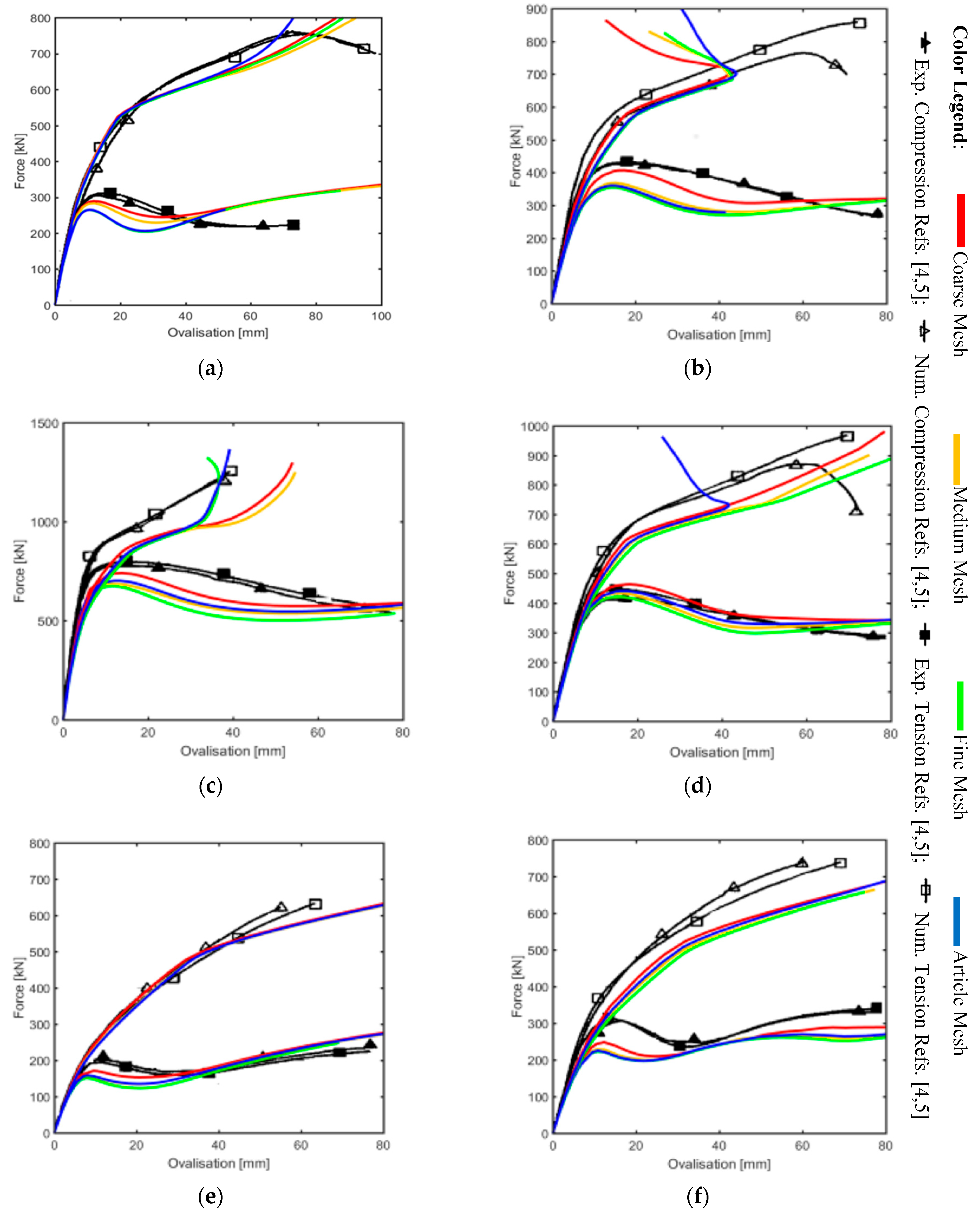
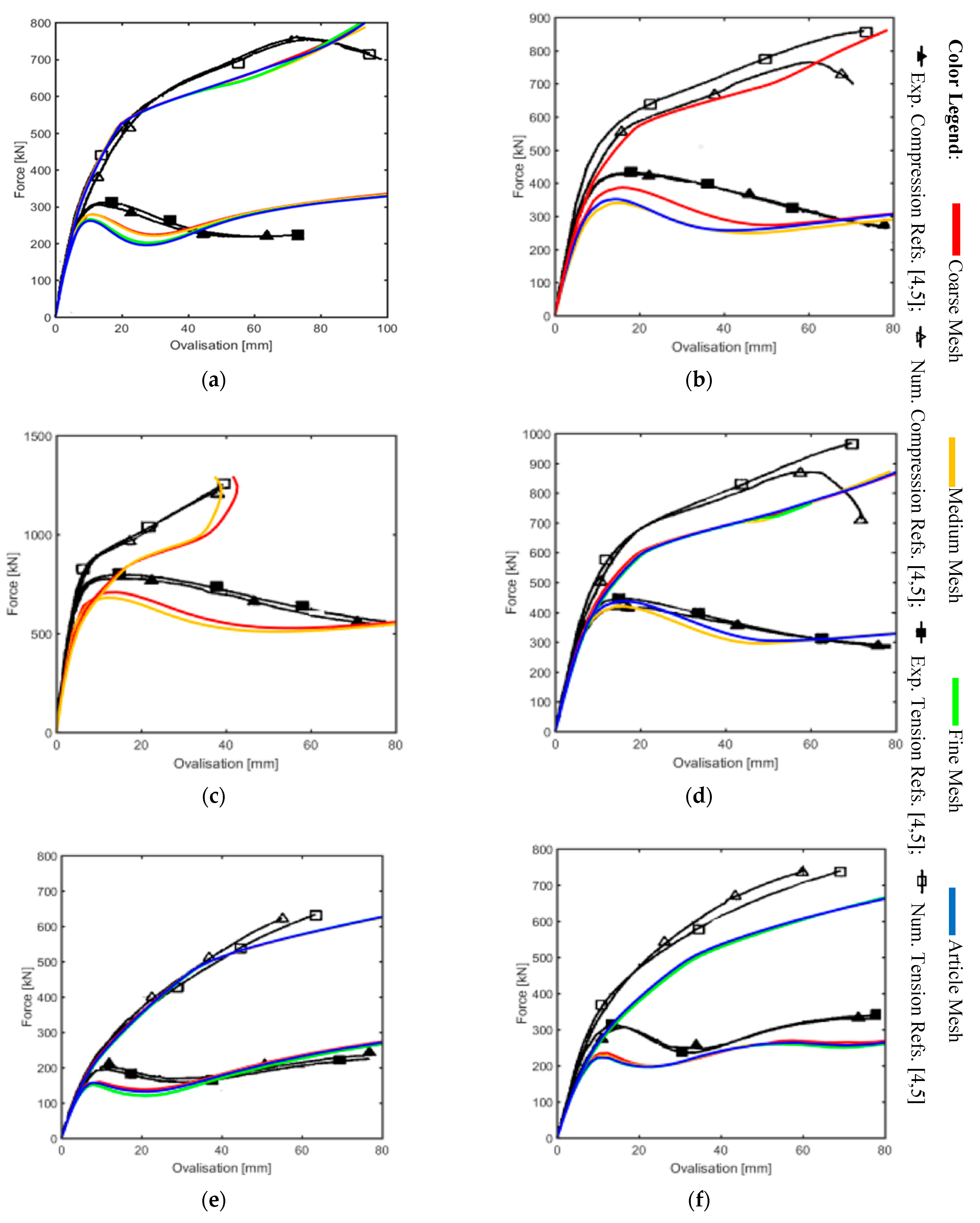
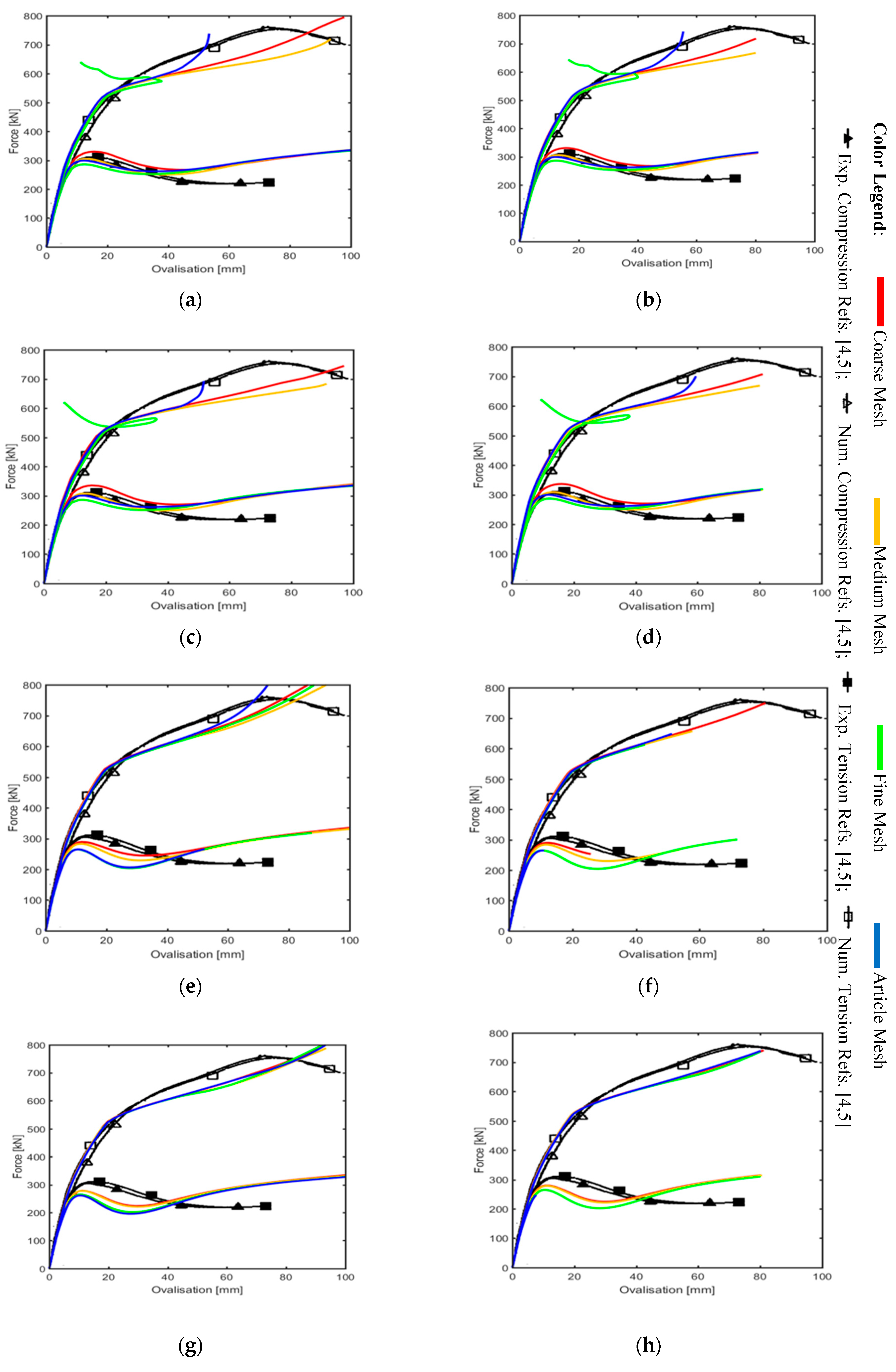
4.1. Curves With Automatic Step Sequence

In this section, the curves are represented in terms of the automatic step sequence. So far, a single step size is applied to the model through the constant step range, and all the four types of elements will be considered (S4R, S4, S8R, and S8R5). For what concerns the figures that will be described, these will represent respectively the Mises stress and PEEQ (Equivalent Plastic Strains) [51] of the specimens.

4.1.1. S4R Element Type

The graphs reported in Figure 5 represent the simulations done for meshes using the S4R element type (that are those given by default from the program), with an automatic step range. It is remarked that the lower curve for each graph refers to the compression specimens (i.e., EX-01 to EX-11 with odd numbers), whereas the higher one represents the tension specimens (i.e., EX-02 to EX-12 with even numbers).

Generally, for all the graphs it is easy to see a good fitting between the reference curves and the present work, especially for the unreinforced cases and for the coarse mesh of collar plate EX-03 and EX-04. The coarse mesh of EX-01, EX-02, EX-03, and EX-04 are depicted in Figure 6a–d.

Unreinforced cases show an inferior maximum stress but are distributed in almost all the chord, whereas the case of collar reinforced plate is characterized by higher maximum value but concentrated in the reinforcement. It is obvious that unreinforced cases have higher values in terms of plastic deformations with respect to the reinforced ones.

The above good fitting is not relatively the case of EX-06, where the present curves are slightly below the reference curves, the marked difference is also influenced by the fact that this is the thicker case, which causes higher values. However, this difference is repeated for all the element types with improvements in S8R, so further discussions are left when the results for these elements will be discussed.

From the curves can be seen two irregular trends, one is the temporary variation in the force values such as for the EX-10, EX-12 with the coarse mesh and slightly in EX-07 and EX-08 with the article mesh; and the second trend is the change in direction of the ovalization (where can be seen a turning back of the curves) such as for fine mesh of EX-01, EX-02, EX-04, EX-06, and EX-08. The first trend is not a model problem but is a consequence of the plasticity of the elements, so it is more related to the FE implementation than the actual modeling, in any case this happens after the maximum ovalization of the reference papers is reached. In addition, this behavior does not affect the specimens in compression. Contrastingly, the second trend is due to the fact that a small part of a corner of a quarter’s brace rises in an unexpected way, as shown in Figure 7b for the fine mesh of the specimen EX-08. It is remarked that this behavior occurs just in the fine mesh, and this might be caused by the fragility of the mesh type (in fact, that does not occur in the S8R, which is the stronger).

4.1.2. S4 Element Type

The major difference between the S4 element type and the previous, the S4R, is that in S4 elements no reduced integration is excepted. This similarity between the S4 and S4R is directly reflected by the results of the load-ovalization curves depicted in Figure 8, from which can be seen there are no big changes from the load-ovalization curves in Figure 5.

Relevant differences can be observed for fine meshes. In the tension cases EX-04 and EX-08 shown in Figure 8b,d, the “hook” is no longer present at the tail of each curve. Moreover, another improvement can be seen in EX-06 in Figure 8c where the reverse curve trend in terms of ovalization is avoided for the medium mesh. While this remains in the fine mesh, such behavior as aforementioned is due to the rise of a part of the chord and this effect is depicted in Figure 7c.

4.1.3. S8R Element Type

In Figure 9 the S8R element is considered. With this type of element, the problem of the drop-in force (due to model exceeding plasticization at the end of the process) of the two previous cases is avoided. But several simulations end before the maximum ovalization (around 80 mm in the references) is reached, especially in the unreinforced case such as the article and coarse mesh of the specimen EX-01, the article mesh of specimen EX-03, and medium and fine mesh of the specimen EX-10.

In the case of the EX-06, that is the one that defers more from the references, but with the S8R element type the differences are reduced. The article mesh solution in Figure 9c has still a different shape with respect to the references but the curves coincide at their ends.

As results in the EX-06 and EX-07 the smaller stress and plasticization can be seen, this is due to the increase in thickness of all the elements, which almost doubled with respect to the other cases. In addition, to this first improvement, for the specimen EX-08 using the S8R element, in the fine mesh the change in direction of the ovalization is also avoided. See Figure 7d where at the end of the simulation no rise of the corner part is present.

4.1.4. S8R5 Element Type

The last element type considered in this research is the S8R5 element type. The S8R5 has just five DOF, this means that there is a simplification respect to the S8R, and this simplification results in the inability to submit all the simulations. The load-ovalization curves of S8R element type depicted in Figure 9 are very close in shape to those of S8R5 reported in Figure 10, but an important issue is solved definitely and no reverse in ovalization is present for all the cases. To notice that was not possible to complete all the simulations because of the complexity of the S8R5 elements type, which does not always allow finding the convergence.

4.2. Curves With Fixed Step Sequence

The plasticization of the T-joint is a key point for the fixed step sequence, since the starting point of the plasticization defines the application of the second step range. From the results of the simulations of EX-01 and EX-02 of the automatic step sequence, the starting period of the plastic behavior of the material of the T-joint is identified. The set of all these values for the two specimens EX-01 and EX-02 are reported in

Table 5. Starting point of the plasticization for Ex-01 and Ex-02 [17].

Element Type Mesh EX-01 and Ex-02	Density Mesh	Starting Point of Plastic Behavior
S4R	Coarse Medium Fine Article	0.009 0.009 0.009 0.009
S4	Coarse Medium Fine Article	0.009 0.009 0.009 0.009
S8R	Coarse Medium Fine Article	0.009 0.006 0.006 0.006
S8R5	Coarse Medium Fine Article	0.009 0.006 0.006 0.006

, which shows that the plasticization starts at the very early stage of the simulations.

So fixed step sequence introduces one more step respect to the automatic one, as in the experimental investigation. For this reason, the simulations have been done for the first two specimens EX-01 and EX-02 as reported for all the four-element type in Figure 11, and once it emerged that no relevant changes in the results are present, it was understood that for this type of model the range application of the load/displacement makes no differences.

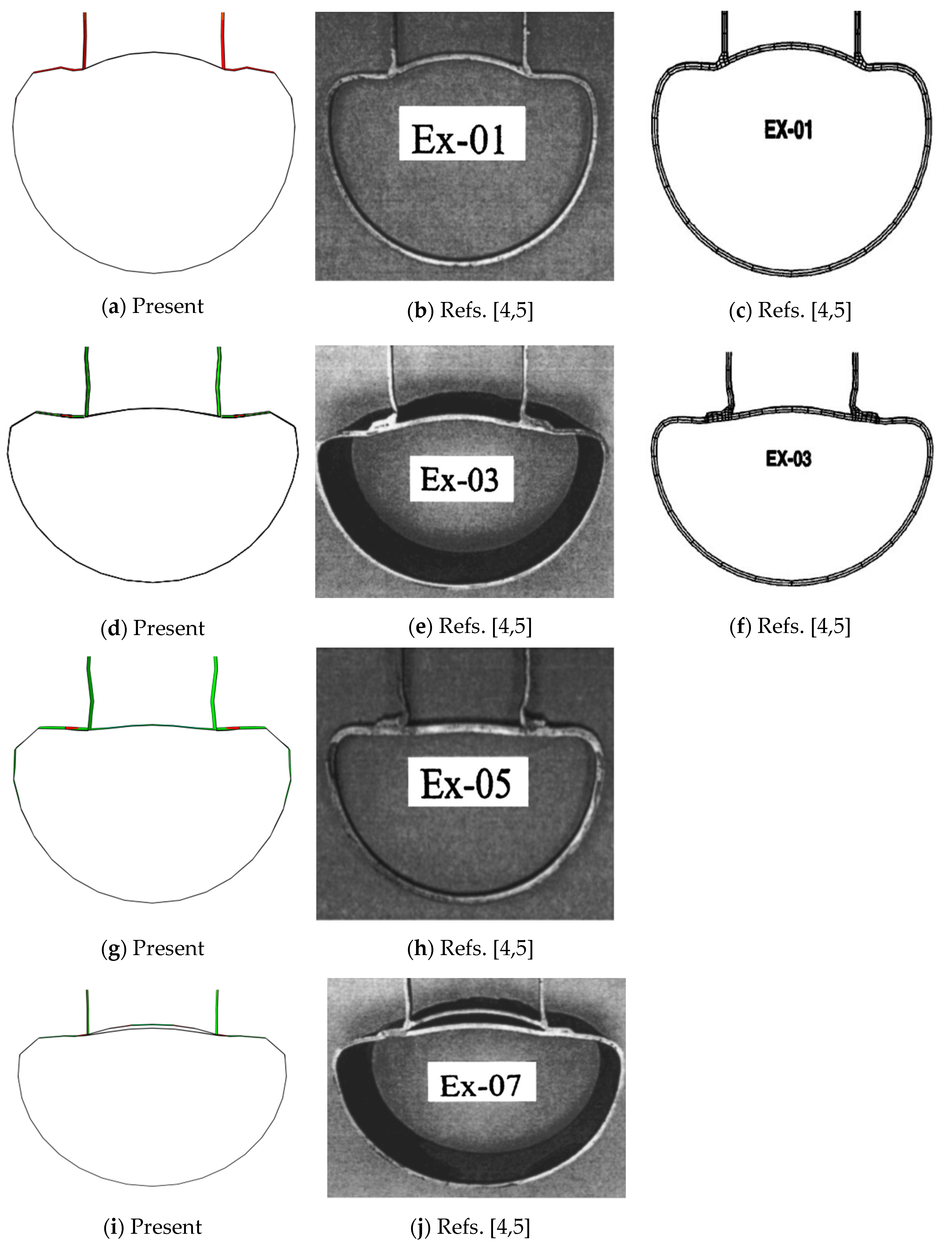
4.3. Deformed Shapes

Other comparisons between the present research and the references [4,5] are discussed in this section. Through considering sections or rings of the tubular elements, from which it is possible to observe the ovalization and associated yield hinges, as well as the separation between the chord and doubler/collar plate.

In the experimental investigation and the numerical simulation [4,5], after the tests were completed, for some of the specimens, sections or “rings” were obtained from the chord and brace. The results have been presented firstly for the specimens with diameter ratio (where $\beta =d_1/d_0$), i.e., from the EX-01 to EX-08, and then for the specimens with $\beta =0.28$, i.e., from the EX-09 to EX-12. Alternatively, in the numerical simulation of var der Vegte et al. [5] the deformed rings, which have been showed, are just some that have the diameter ratio $\beta =0.54$. Therefore, some gaps can be seen in the representation of the rings for what concern to the reference [4,5].

In the following the ovalization shapes will be shown, compared with the papers’ results, where these are present. The same experimental subdivision will be considered. The research simulations exceed the length of this paper’s simulation in most cases, whereby in the section will be taken from the same ovalization as literature cases. In addition, in this paper for further investigations of the shapes will be selected the ones that have the best fit in the load-ovalization curves.

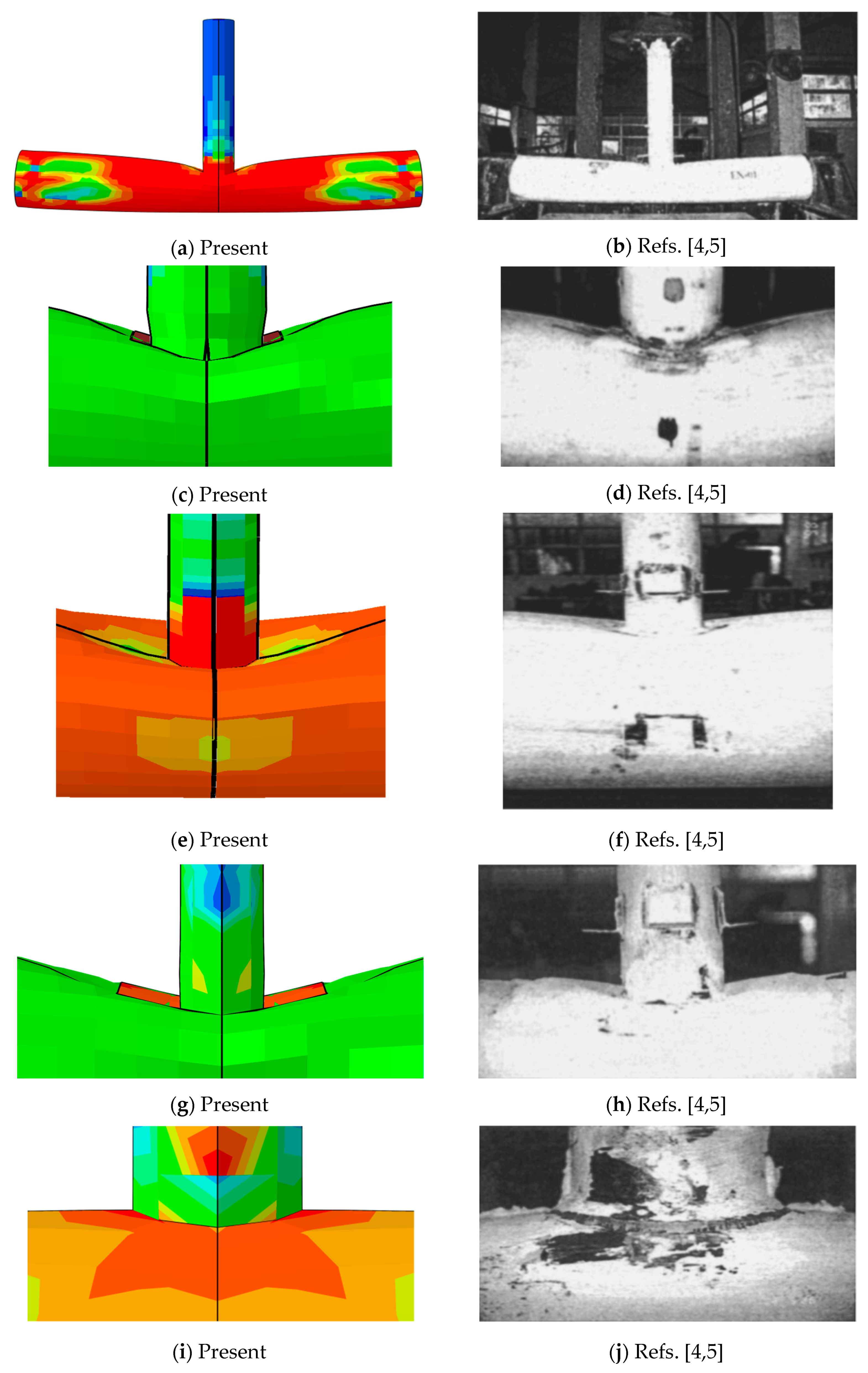
4.3.1. Failure of the Specimens with $\beta =0.54$ under Compression

Specimens under compression in the brace element with diameter ratio equal to 0.54 are EX-01, EX-03, EX-05, and EX-07. These are all represented in the experimental investigation, whereas in the numerical simulation reference to EX-05 is missing.

Specimen EX-01 

Figure 12a,b shows the overall view of the unreinforced specimens of the Experimental Case (EC) (reference figures from [4,5]) and the Research Case (RC) (the present simulations). The present contour plots represent the MISES stresses.

Figure 13a–c shows the sliced ring (chord and short portion of brace) from specimen EX-01, and here, different from the overall view, the case of Numerical Case (NC) (FE simulation from the references [4,5]) is also present. From the paper’s results can be seen the two yield hinges adjacent to brace-chord intersection become clear, while in the research case, however, this cannot be seen and the shape does not follow the same trend. As aforementioned the step taken is at ovalization 100 mm, which corresponds to the period 0.672 of 1 Abaqus simulation time period.

Specimen EX-03 

For the specimen EX-03 the papers presented only the sliced result. Figure 13d–f shows the sliced ring of specimen EX-03. Between this specimen and the previous one it can be immediately noticed the significant strength enhancement offered by the collar reinforcement to the chord section for EX-03. The step taken here is at ovalization 80 mm, which corresponds to the period 0.476 of 1 Abaqus simulation time period.

Specimen EX-05 

Figure 12c,d shows the detail of the chord indentation side view of the reinforced specimen EX-05; also, here the work case is showed in form of MISES stress, where plastic deformation is near the intersection chord-brace, whereas the chord bottom part remained relatively straight with no deformation and no stress concentration. Figure 13g,h shows the sliced ring from specimen EX-05, here the NC was not available in the results. The bending in this case is more severe than that of specimen EX-03, some results of the relatively higher strength of the chord, as can be seen in load-ovalization curves. Ovalization 80 mm corresponds to the period 0.614 of 1 Abaqus simulation time period.

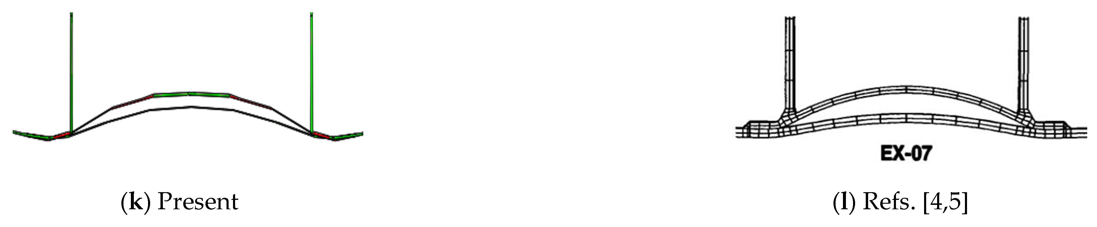
Specimen EX-07 

As far as EX-07 is concerned, the papers presented only the sliced result, as depicted in Figure 13i,j. The separation from the chord outer surface of the doubler plate (which at the original shape fits the chord perfectly) can be observed. As can be seen in Figure 13k,l, RC also has this effect but with no such emphasis as in the papers’ cases. This behavior is due to the fact while the brace compresses the chord, the wall of the latter has a different rotation with respect to the reinforcement; in the FE model the modeling of the contact and ties have played a fundamental role. In this the ovalization 80 mm corresponds to the period 0.531 of 1 Abaqus simulation time period.

4.3.2. Failure of the Specimens with $\beta =0.54$ under Tension

In the following, the specimens under tension in the brace element with diameter ratio equal to 0.54 will be considered. These specimens are EX-02, EX-04, EX-06, and EX-08. Here the experimental investigation results are given for EX-04, EX-06, and EX-08, while in the numerical simulation just the EX-08 is given.

During the experimental test, some specimens buckle such as EX-02 and EX-04; while for the numerical simulations the buckling was not taken into account. Also, in the present research, the buckling is not covered, but is left as future development.

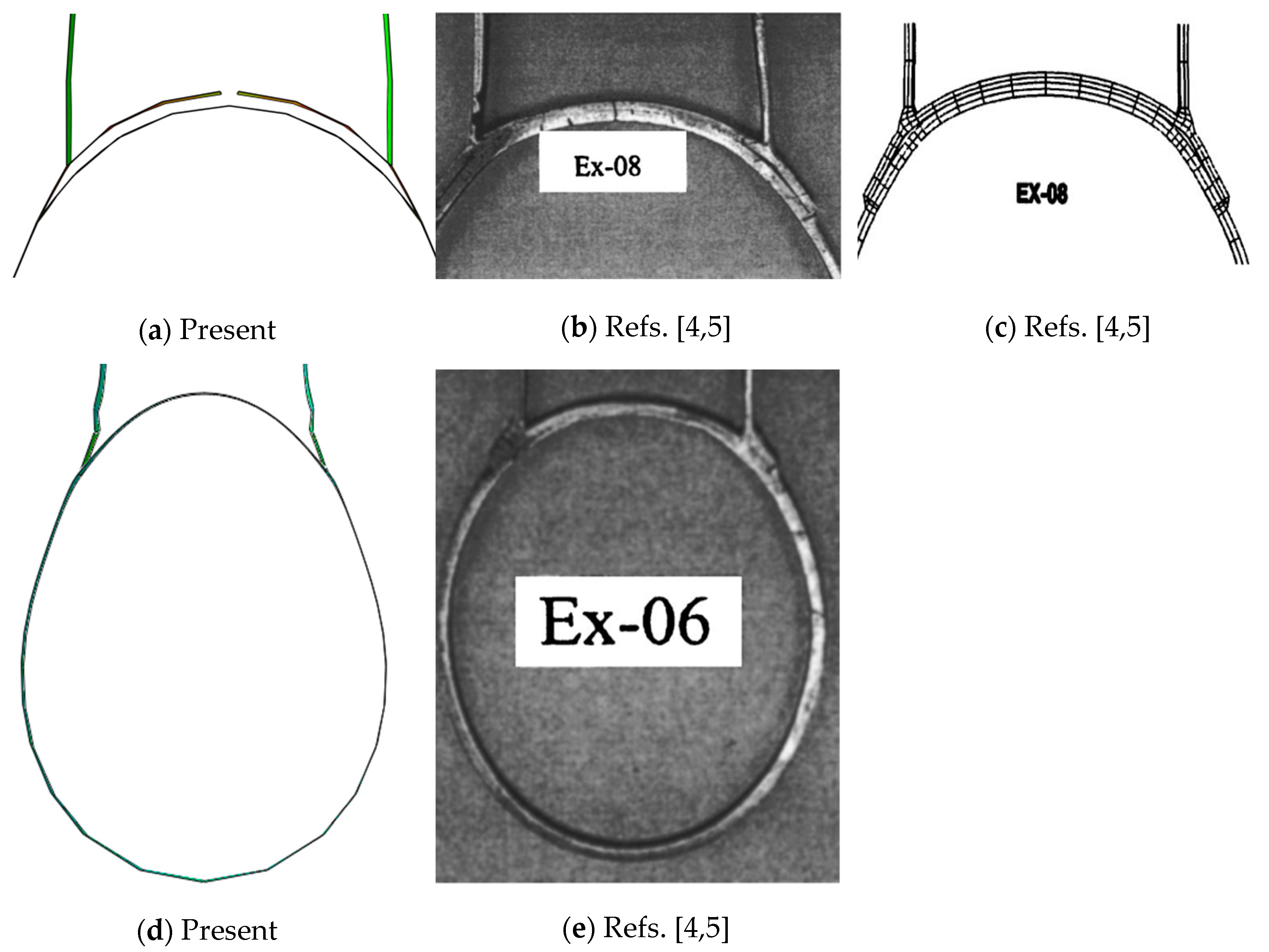
Specimens with Buckling EX-02, EX-04, and EX-08 

Even if in this research the buckling is not taken into account, due to the initial purpose which is that of building a reliable model made of shell elements, a good match has been found in the load-ovalization curves as can be seen also here in the deformed shapes of the specimen where the buckling occurred in the physical experiment [4]. However, the buckling was also not considered in the previous numerical simulation [5], and the results in terms of deformed shape from the numerical simulation were not provided.

EX-02, EX-04, and 08 are the three cases where the specimens buckle. The doubler plate specimen EX-08 subjected to brace tension has a similar pattern to the EX-04, with pronounced chord plasticization. In Figure 14a–c the separation of the doubler plate from the chord at the brace-doubler intersection is illustrated. This separation can be seen both in the reinforced and unreinforced case, also without considering the buckling effect.

Specimen EX-06 

EX-06 is the thicker specimen with collar reinforcement subjected to brace tension. Its deformed shape is shown in Figure 14d,e. For this specimen the experimental test was terminated after the tensile capacity of the actuator was reached at 1200 kN, in RC the simulation also stops earlier, and at the end of time period 1 the ovalization is equal to 38 mm instead of 80 mm in the references [4,5].

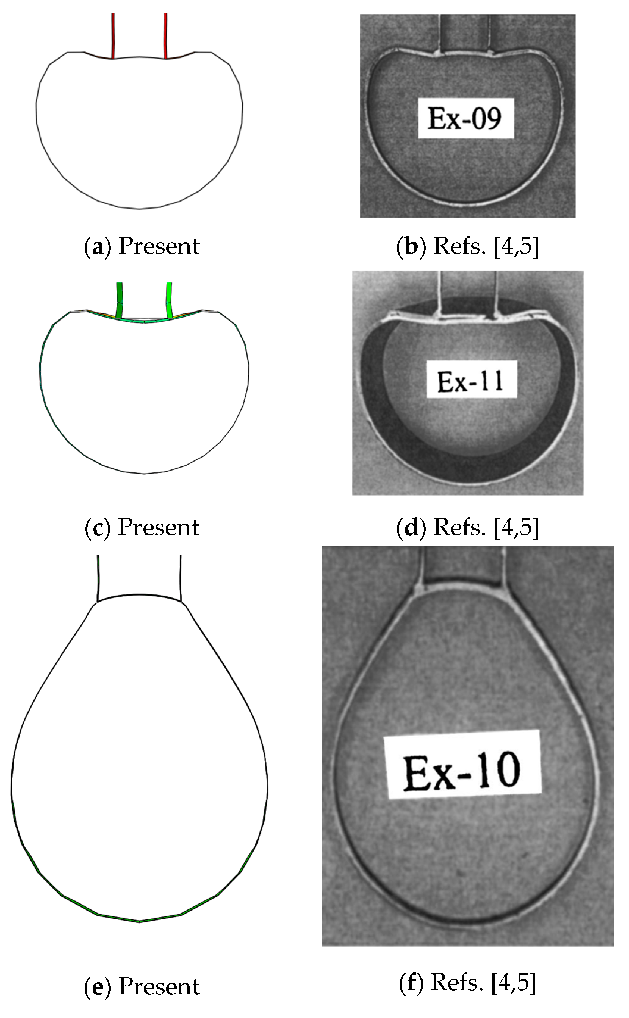
4.3.3. Failure of the Specimens with $\beta =0.28$ under Compression

In the following specimens under compression with $\beta =0.28$ are shown, and this is the case of EX-09 and EX-11. For both cases the NC does not show any result, so they will be compared only for the EC with the present research.

Specimen EX-09 

Figure 12e,f shows the localized indentation of the chord of unreinforced specimen EX-09 subjected to compression, which has a similar behavior of the respective specimen with higher diameter ratio EX-01. For the sake of comparison, Figure 15a,b presents its sliced ring. The step taken here is at ovalization 80 mm, which corresponds to the period 0.450 of 1 Abaqus simulation time period.

Specimen EX-11 

Figure 12g,h shows the localized indentation of the chord of the reinforced specimen EX-11 subjected to compression; besides the appreciable indentation at the intersection area, the doubler plate is observed to bulge out of its plane. Contrastingly, Figure 15c,d presents its sliced ring. The step taken here is at ovalization 80 mm, which corresponds to the period 0.537 of 1 Abaqus simulation time period.

4.3.4. Failure of the Specimens with $\beta =0.28$ under Tension

In the following the last two specimens examined are EX-10 and EX-12, with small ratio but subjected to tension. Only EX-10 will be showed here, since EX-12 in the experimental investigation was stopped due to brittle failure that occurred through punching shear fracture of the brace out of the doubler plate.

Specimen EX-10 

Figure 12i,j shows a detailed view of the brace-chord intersection of the unreinforced specimen EX-10 subjected to brace tension; also, after severe plasticization, the joint exhibited brittle shear failure of the chord wall at one side of the intersection. In the EC the focus is at the weld zone that is not present in the RC. Alternatively, Figure 15e,f presents its sliced rings, which shows very similar shapes. The time step taken here is at ovalization 80 mm, for a period 0.443 of 1 Abaqus simulation time period.

5. Summary and Conclusions

The FE analyses with the use of shell elements in this research have been directed to simulate the static behavior of a set of 12 unreinforced and reinforced test cases, on uniplanar T-joints under axial brace load carried out by Choo et al. [4]. In addition to the investigation conducted by Choo et al. [4], the numerical simulation of var der Vegte et al. [5] has been taken into account. Even though a FE study is already present, there the authors have decided to use the more computationally expensive 3-D model made by solid elements. The present research tries to solve the issues faced in [5] and sheds light on the importance of the mechanical data in FE modeling. Some peculiar data that are missing in the reference papers were discussed.

The results are presented in terms of restraining force versus ovalization of the chord under the applied force and also in terms of deformed shapes, by considering sections or rings of the tubular elements. Based on the results presented in the previous sections, where several parametric settings have been considered, the following conclusions and considerations can be made.

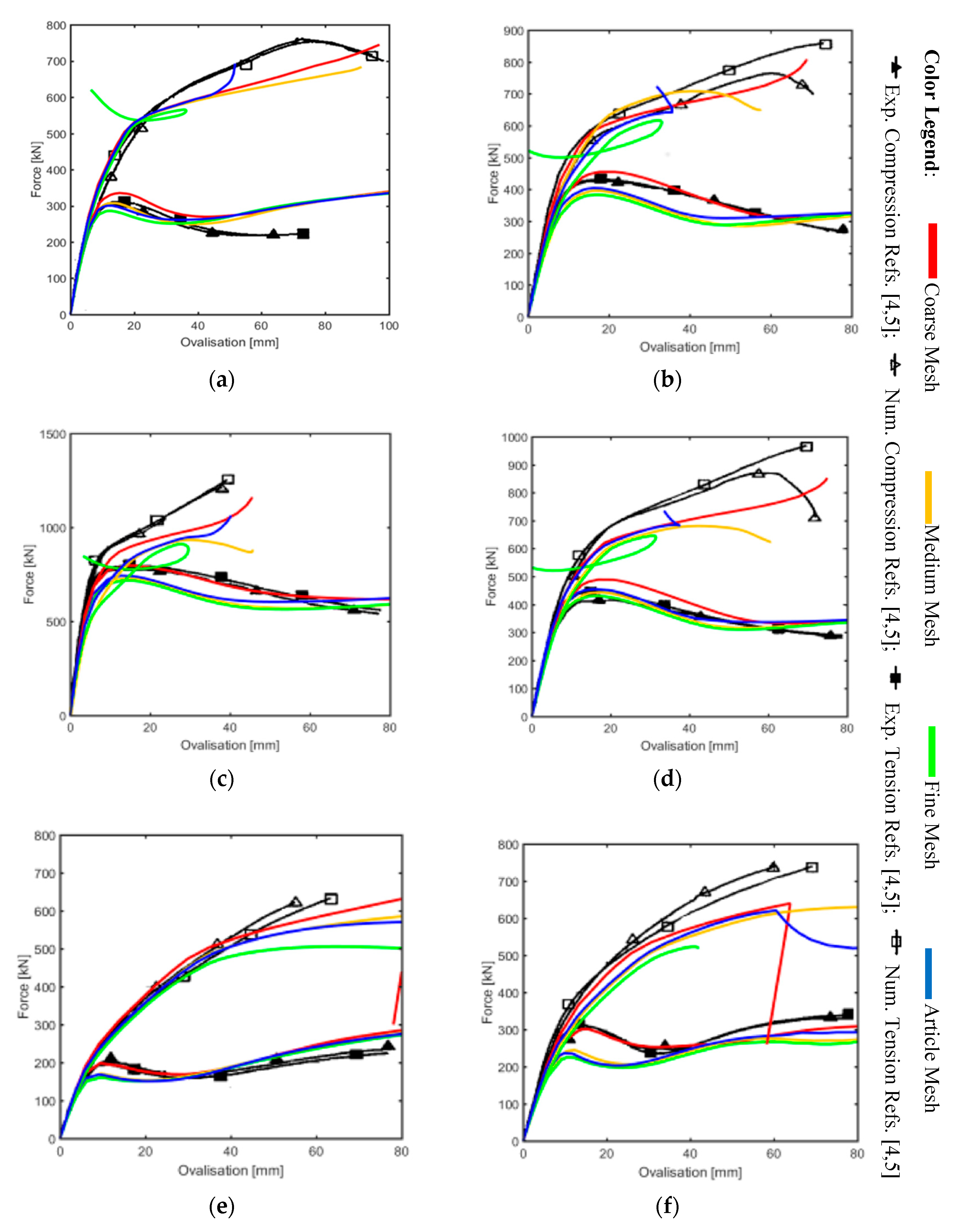
• The difference in terms of load application does not affect the results in relevant way, since the results obtained by the automatic step sequence (i.e., unique stroke range) and those obtained by the fixed step sequence (i.e., two stroke ranges as in the experimental investigation) for the first two specimens are almost the same, except in some cases of the fixed step where it was not possible to find the convergence for all, due to the complexity caused by the double step. Therefore, the automatic step sequence was considered for the remaining samples that besides being simpler also allows an easier convergence.
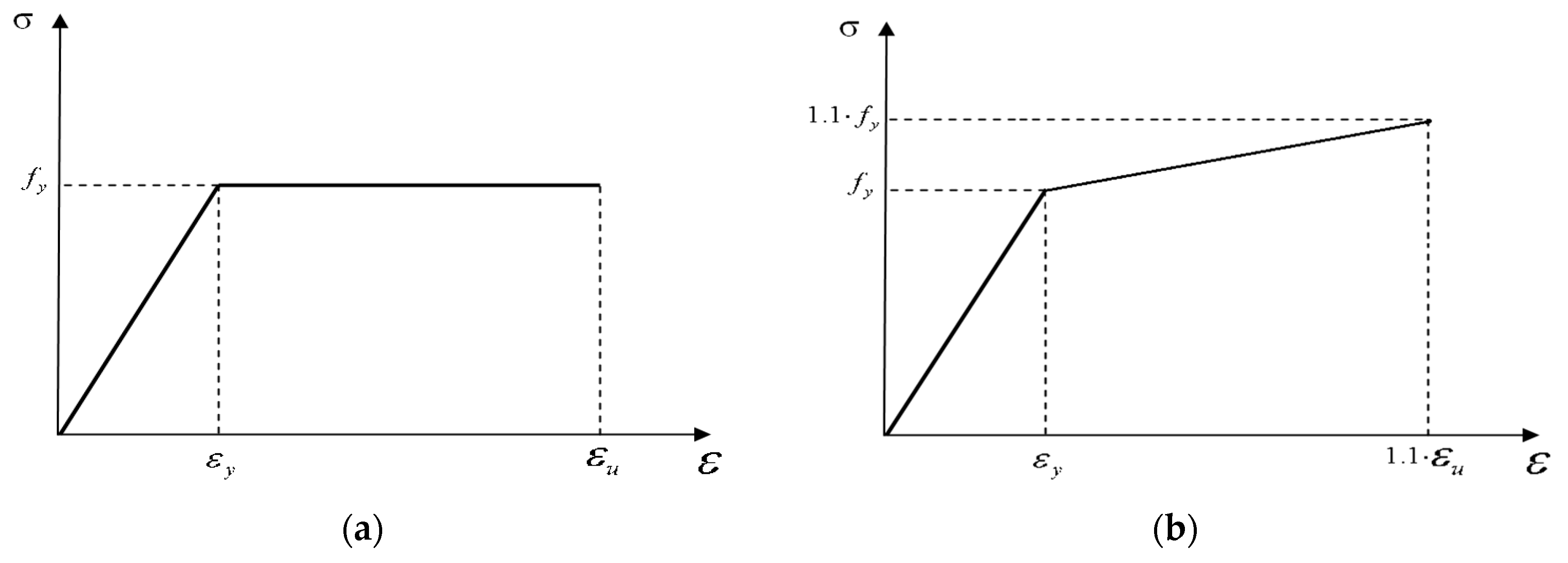
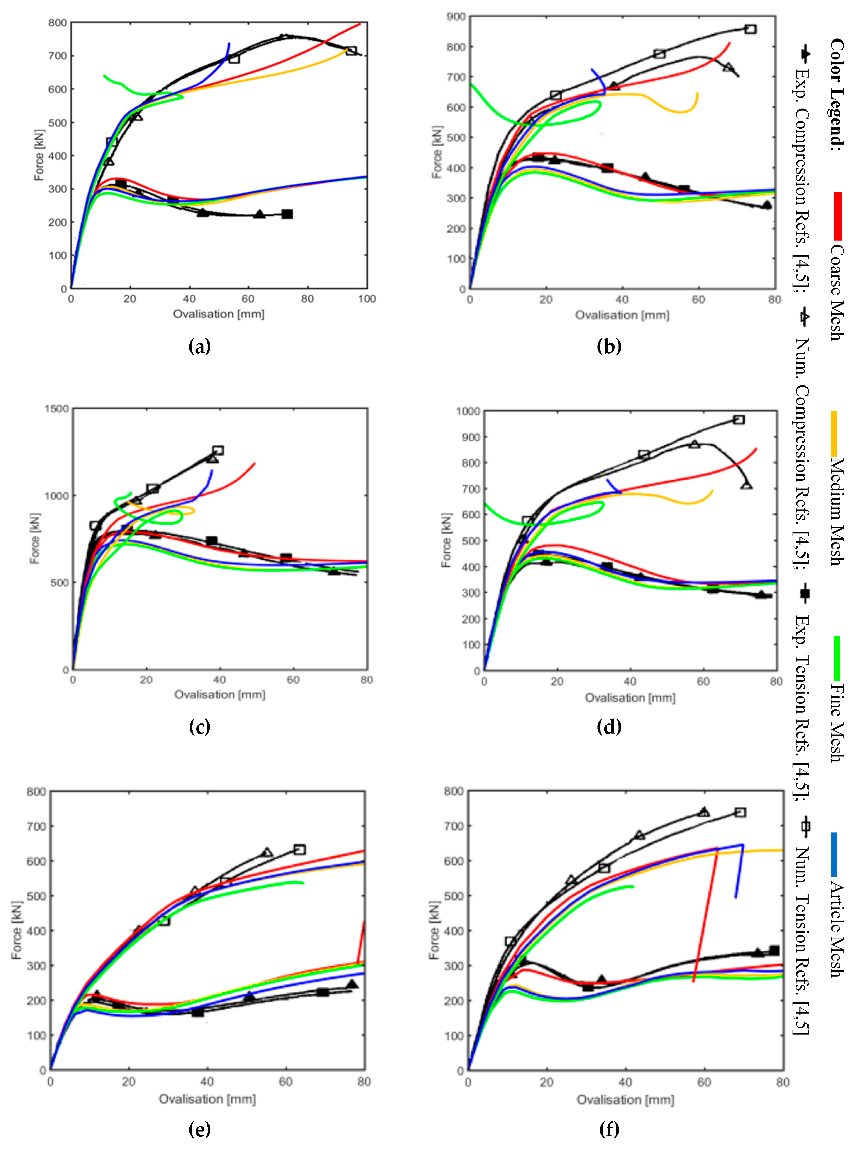
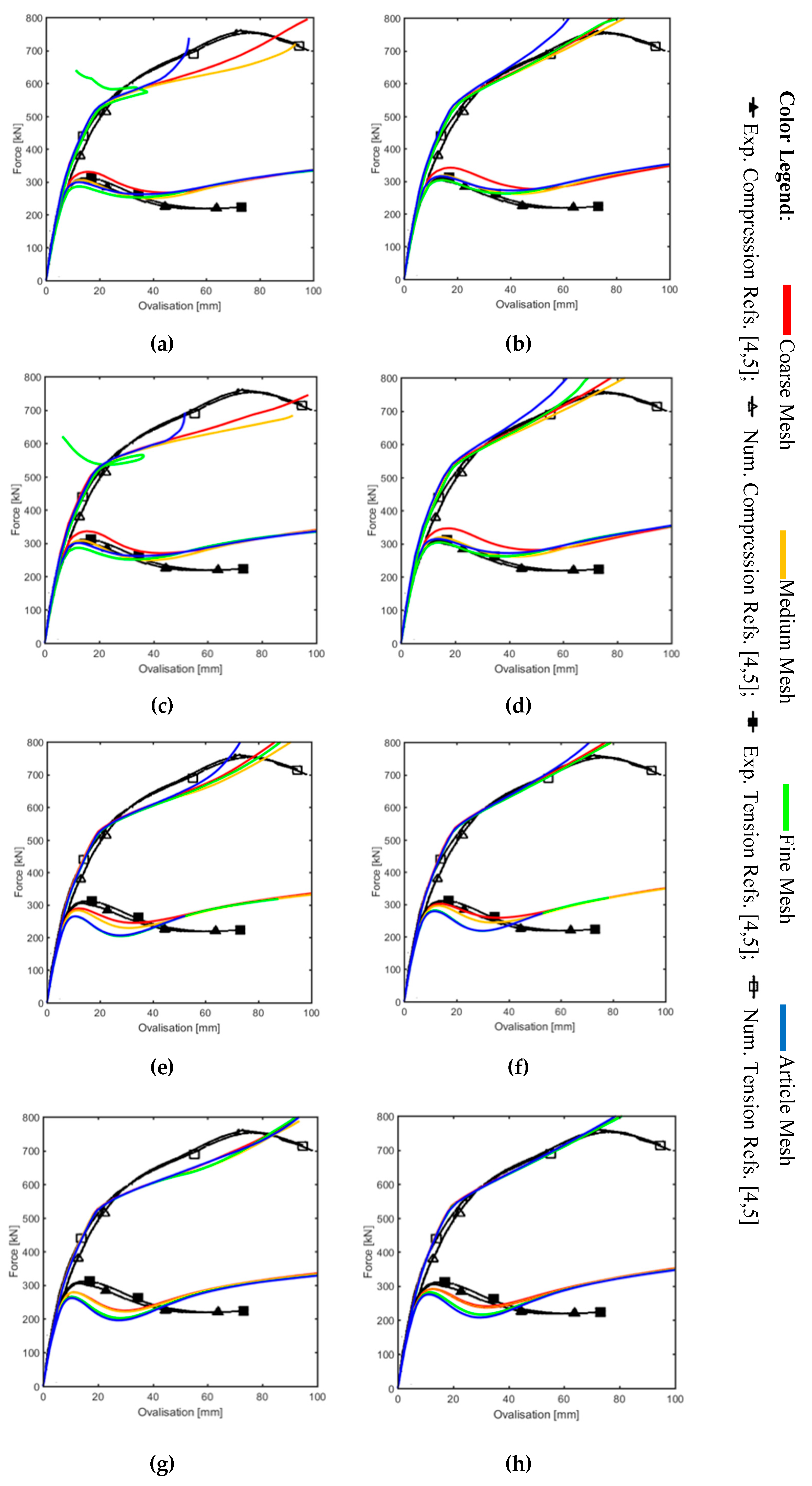
• Automatic step sequence and the true stress-strain relationship without hardening after the peak load were considered. For these settings, four different mesh densities (coarse, medium, fine, and article) each one analyzed with four-element types (S4R, S4, S8R, and S8R5) were analyzed, respectively. Generally, it was possible to see that all load-ovalization curves fit quite well in the initial (linear) part with the reference investigation, and then go slightly below in the post-peak, and finally to converge almost in final value. In the first group of element types, i.e., S4R and S4, it can be seen that there is an abnormal shape of the curves, with the reverse of the ovalization, when the elements size of the mesh used are relatively small such as in the medium and fine mesh. This is valid when $\beta =0.54$, i.e., the diameter of the brace is more than half of the chord one. While if this ratio is decreased to $\beta =0.28$ this does not occur. In contrast, the second group of element types with a higher number of nodes solves the issue of the change in direction of the ovalization for all the cases, even though a higher number of nodes leads to no convergence for some specimens.
• Due to the fact that the automatic step sequences, with no hardening simulations, have the relevant and complete data, these were compared to the references by cutting rings from the center of the chord of each specimen. The ring of the research shows a perfect matching to the experimental case under compression. In the research study, as in the numerical reference, the buckling that occurs in some of the tension cases of the experimental research was not considered. However, the shapes obtained by this research kept good accordance, even in the specimens where buckling occurred.
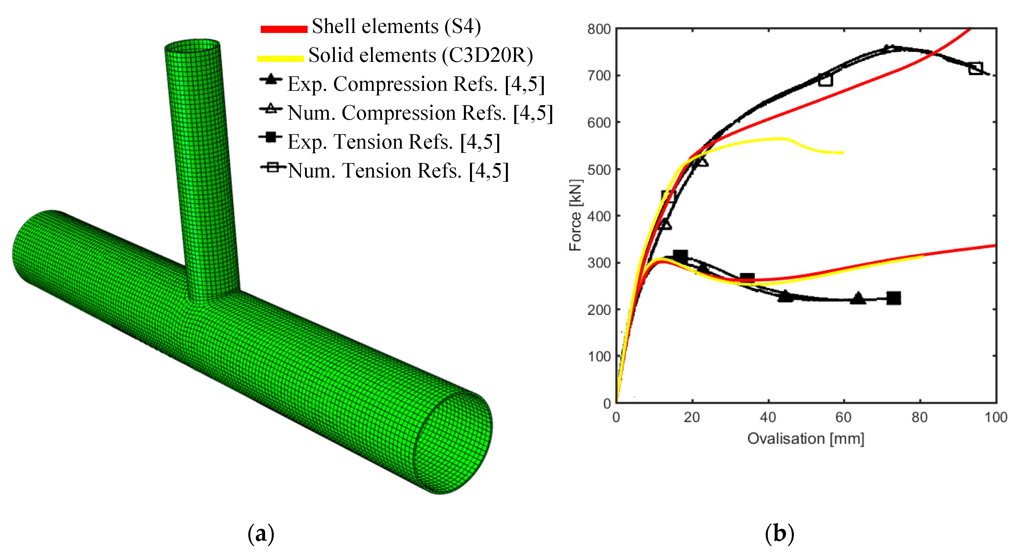
• Although the reliability of shell elements is the object of this research, a 3-D model with the same setting used by var der Vegte et al. [5] was built to verify the reliability of the preliminary parameters considered in the model with those of the numerical simulation [5], since assumptions were done in the first stage due to lack in the data in the reference papers. From the results of the 3-D model of this study, as depicted in Figure 16a, the load-ovalization curves in Figure 16b have been obtained where almost similar shapes and characteristics of the main model made by shells with S4 element type can be seen. Thus, it is possible to deduce that some relevant data are missing in the paper.
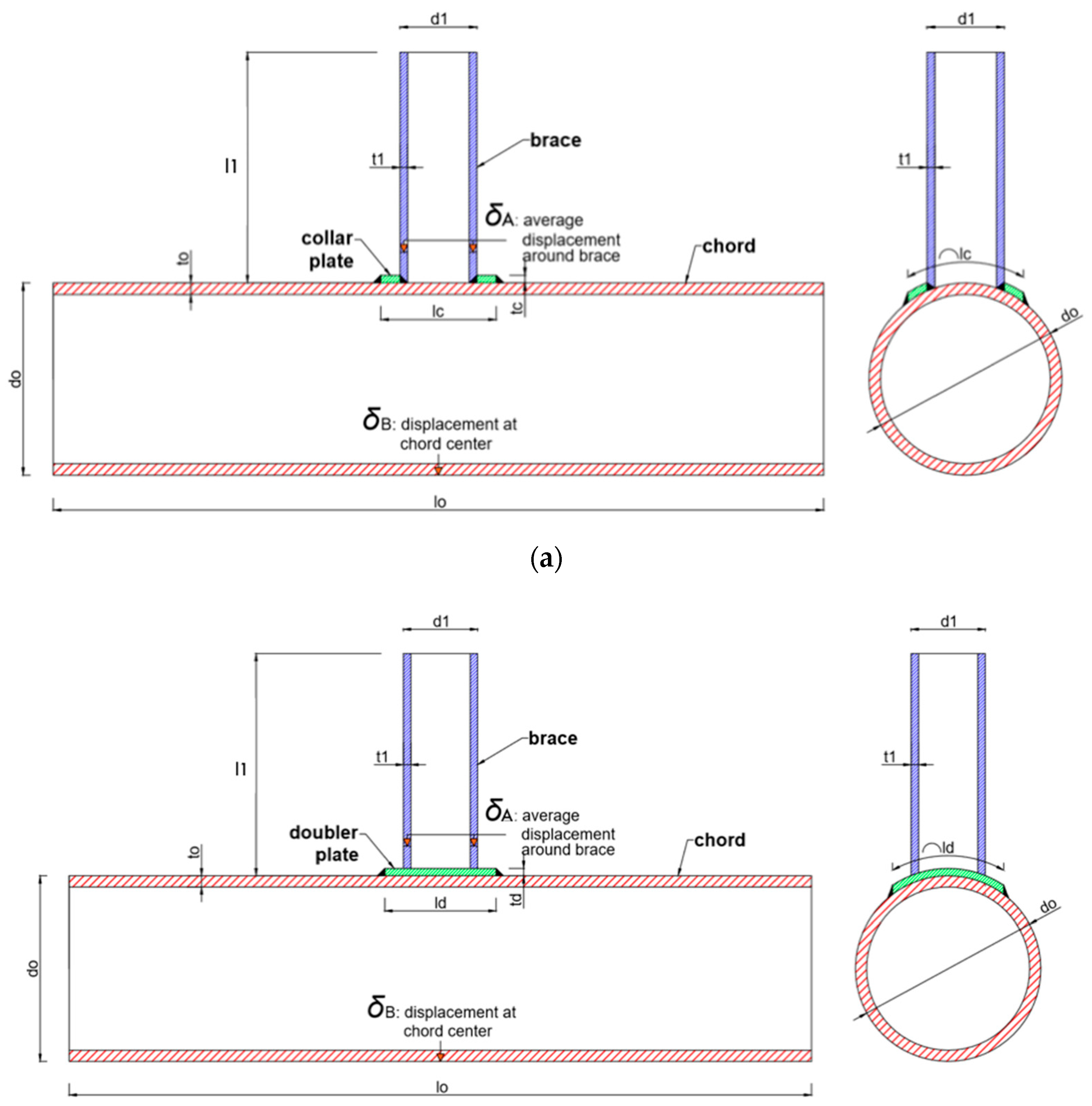
• The model considered in this research is able to show comparable strength characteristics as in [4,5]. In fact, the T-joints considered in this study show a great improvement in terms of strength of the specimen reinforced by doubler plate or a collar plate as compared to the strength of the unreinforced joints. An enhancement of almost 40% was reached for $\beta =0.54$ as in the experimental case, but a smaller value was found for $\beta =0.28$ where the research value is five per cent smaller than the experimental one of sixteen percent. Therefore, it can be said that the two types of reinforcement have the capacity to distribute the brace axial load to a larger region of the chord, with consequent improvement in terms of strength enhancement.
• Through the use of shell elements instead of the more expensive (in terms of computational cost) solid elements, the contact problem and the introduction of the element thickness have been solved. It turned out that shell elements with 8 nodes and reduced integration are suitable for this type of structures; this type of elements gives a reliable solution already starting from coarse meshes. Whereas the S4R elements type given by default from the software gives less precise results.
• The missing data in the reference papers have inevitably lead to some differences in the results, partially solved by the use of a different true stress-strain relationship. However, due to the good agreement between the research and the experimental results, the former can be developed through parametric studies to extend the above considerations to different types of joints. Moreover, the present research can be considered for studies involving composite materials as reinforcing phase for damaged or weak joints.

6. Future Developments

The authors analyzed, in the first instance, T-joints with shell elements. Since small deviations have been noticed, solid elements models have been generated to test the same joints as in [5]. However, the following conclusions are drawn to a future development of the present paper, which will consider a deep analysis of the mechanical properties used in the experimental testing. As a matter of fact, as a preliminary study the solid models are comparable to the shell ones by considering the same input data.

The differences between the reference studies [4,5] and the present ones are in the “large deformation” part of the curves. The linear elastic branch is so small that it cannot be seen in the plots, but it is very clear that the curves have two segments, and both are nonlinear.

Due to this change, which seemed to be a consequence of the previous assumption done for the material properties, where the true stress-true strain relationship was taken as elastic-perfectly plastic model reported in Figure 2a. Hence, it has been decided to introduce a hardening of 10% in the true stress-strain relationship for the first two specimens as reported in Figure 2b, differently to what was written in the reference paper [5].

The outcome of this setting, as depicted in Figure 17, gives for the tension cases a very close match of the curves for almost 90% of each simulation, while in compression some differences can still be noted. True strain-stress relationship closer to the real behavior of the steel material (left to future studies) can solve this last deference.

References

- Moffat, D.G.; Kruzelecki, J.; Blachut, J. The effects of chord length and boundary conditions on the static strength of a tubular T-joint under brace compression loading. Mar. Struct. 1996, 9, 935–947. [Google Scholar] [CrossRef]
- Choo, Y.S.; Qian, X.D.; Foo, K.S. Static strength variation of thick-walled CHS X-joints with different included angles and chord stress levels. Mar. Struct. 2004, 17, 311–324. [Google Scholar] [CrossRef]
- Lee, M.M.K.; Llewelyn-Parry, A. Strength prediction for ring-stiffened DT-joints in offshore jacket structures. Eng. Struct. 2005, 27, 421–430. [Google Scholar] [CrossRef]
- Choo, Y.S.; van der Vegte, G.J.; Zettlemoyer, N.; Li, B.H.; Liew, J.Y.R. Static strength of T-joints reinforced with doubler or collar plates. I: Experimental investigations. J. Struct. Eng. 2005, 131, 119–128. [Google Scholar] [CrossRef]
- van der Vegte, G.J.; Choo, Y.S.; Liang, J.X.; Zettlemoyer, N.; Liew, J.Y.R. Static Strength of T-joints reinforced with doubler or collar plates. II: Numerical investigations. J. Struct. Eng. 2005, 131, 129–138. [Google Scholar] [CrossRef]
- Yang, J.; Shao, Y.; Chen, C. Static strength of chord reinforced tubular Y-joints under axial loading. Mar. Struct. 2012, 29, 226–245. [Google Scholar] [CrossRef]
- Ozyurt, E.; Wang, Y.C.; Tan, K.H. Elevated temperature resistance of welded tubular joints under axial load in the brace member. Eng. Struct. 2014, 59, 574–586. [Google Scholar] [CrossRef]
- Chen, Y.; Feng, R.; Wang, C. Tests of steel and composite CHS X-joints with curved chord under axial compression. Eng. Struct. 2015, 99, 423–438. [Google Scholar] [CrossRef]
- Lie, S.T.; Li, T.; Shao, Y.B.; Vipin, S.P. Plastic collapse load prediction of cracked circular hollow section gap K-joints under in-plane bending. Mar. Struct. 2016, 50, 20–34. [Google Scholar] [CrossRef]
- Qu, H.; Li, A.; Huo, J.; Liu, Y. Dynamic performance of collar plate reinforced tubular T-joint with precompression chord. Eng. Struct. 2017, 141, 555–570. [Google Scholar] [CrossRef]
- Zhu, L.; Yang, K.; Bai, Y.; Sun, H.; Wang, M. Capacity of steel CHS X-joints strengthened with external stiffening rings in compression. Thin-Walled Struct. 2017, 115, 110–118. [Google Scholar] [CrossRef]
- Đuričić, Đ.; Aleksić, S.; Šćepanović, B.; Lučić, D. Experimental, theoretical and numerical analysis of K-joint made of CHS aluminium profiles. Thin-Walled Struct. 2017, 119, 58–71. [Google Scholar] [CrossRef]
- Lan, X.; Huang, Y.; Chan, T.-M.; Young, B. Static strength of stainless steel K- and N-joints at elevated temperatures. Thin-Walled Struct. 2018, 122, 501–509. [Google Scholar] [CrossRef]
- Qu, S.; Wu, X.; Sun, Q. Experimental study and theoretical analysis on the ultimate strength of high-strength-steel tubular K-Joints. Thin-Walled Struct. 2018, 123, 244–254. [Google Scholar] [CrossRef]
- Li, X.; Zhang, L.; Xue, X.; Wang, X.; Wang, H. Prediction on ultimate strength of tube-gusset KT-joints stiffened by 1/4 ring plates through experimental and numerical study. Thin-Walled Struct. 2018, 123, 409–419. [Google Scholar] [CrossRef]
- Feng, R.; Chen, Y.; Wei, J.; He, K.; Fu, L. Behaviour of grouted stainless-steel tubular X-joints with CHS chord under axial compression. Thin-Walled Struct. 2018, 124, 323–342. [Google Scholar] [CrossRef]
- Ouakka, S. On the Static Strength of Reinforce Joints. Master’s Thesis, University of Bologna, Bologna, Italy, 2017. [Google Scholar]
- Lotsberg, I. On stress concentration factors for tubular Y- and T-Joints in frame structures. Mar. Struct. 2011, 24, 60–69. [Google Scholar] [CrossRef]
- Osawa, N.; Yamamoto, N.; Fukuoka, T.; Sawamura, J.; Nagai, H.; Maeda, S. Study on the preciseness of hot spot stress of web-stiffened cruciform welded joints derived from shell finite element analyses. Mar. Struct. 2011, 24, 207–238. [Google Scholar] [CrossRef]
- Lotfollahi-Yaghin, M.A.; Ahmadi, H. Geometric stress distribution along the weld toe of the outer brace in two-planar tubular DKT-joints: Parametric study and deriving the SCF design equations. Mar. Struct. 2011, 24, 239–260. [Google Scholar] [CrossRef]
- Cheng, B.; Qian, Q.; Zhao, X.-L. Stress concentration factors and fatigue behavior of square bird-beak SHS T-joints under out-of-plane bending. Eng. Struct. 2015, 99, 677–684. [Google Scholar] [CrossRef]
- Pradana, M.R.; Qian, X.; Swaddiwudhipong, S. Simplified Effective Notch Stress calculation for non-overlapping circular hollow section K-Joints. Mar. Struct. 2017, 55, 1–16. [Google Scholar] [CrossRef]
- Cheng, B.; Li, C.; Lou, Y.; Zhao, X.-L. SCF of bird-beak SHS X-joints under asymmetrical brace axial forces. Thin-Walled Struct. 2018, 123, 57–69. [Google Scholar] [CrossRef]
- Xia, J.; Chang, H.; Goldsworthy, H.; Bu, Y.; Lu, Y. Axial hysteretic behavior of doubler-plate reinforced square hollow section tubular T-joints. Mar. Struct. 2017, 55, 162–181. [Google Scholar] [CrossRef]
- Gao, F.; Guo, X.-Z.; Long, X.-H.; Guan, X.-Q.; Zhu, H.-P. Hysteretic behaviour of SHS brace-H-shaped chord T-joints with transverse stiffeners. Thin-Walled Struct. 2018, 122, 387–402. [Google Scholar] [CrossRef]
- Ahmadi, H.; Nejad, A.Z. Geometrical effects on the local joint flexibility of two-planar tubular DK-joints in jacket substructure of offshore wind turbines under OPB loading. Thin-Walled Struct. 2017, 114, 122–133. [Google Scholar] [CrossRef]
- Tong, L.W.; Xu, G.W.; Yang, D.L.; Mashiri, F.R.; Zhao, X.L. Fatigue behavior and design of welded tubular T-joints with CHS brace and concrete-filled chord. Thin-Walled Struct. 2017, 120, 180–190. [Google Scholar] [CrossRef]
- Dong, W.; Moan, T.; Gao, Z. Long-term fatigue analysis of multi-planar tubular joints for jacket-type offshore wind turbine in time domain. Eng. Struct. 2011, 33, 2002–2014. [Google Scholar] [CrossRef]
- Jiang, W.Q.; Wang, Z.Q.; McClure, G.; Wang, G.L.; Geng, J.D. Accurate modeling of joint effects in lattice transmission towers. Eng. Struct. 2011, 33, 1817–1827. [Google Scholar] [CrossRef]
- Cheng, S.; Becque, J. A design methodology for side wall failure of RHS truss X-joints accounting for compressive chord pre-load. Eng. Struct. 2016, 126, 689–702. [Google Scholar] [CrossRef]
- Ahmed, A.; Qian, X. A toughness-based deformation limit for fatigue-cracked X-joints under in-plane bending. Mar. Struct. 2015, 42, 33–52. [Google Scholar] [CrossRef]
- Liu, B.C. Experimental analysis of tubular joints using white light speckle method. Mar. Struct. 1995, 8, 81–91. [Google Scholar] [CrossRef]
- Pey, L.P.; Soh, A.K.; Soh, C.K. Partial implementation of compatibility conditions in modeling tubular joints using brick and shell elements. Finite Elem. Anal. Des. 1995, 20, 127–138. [Google Scholar] [CrossRef]
- Mackerle, J. Fastening and joining: Finite element and boundary element analyses—A bibliography (1992–1994). Finite Elem. Anal. Des. 1995, 20, 205–215. [Google Scholar] [CrossRef]
- Mackerle, J. Fatigue analysis with finite and boundary element methods a bibliography (1993–1995). Finite Elem. Anal. Des. 1997, 24, 187–196. [Google Scholar] [CrossRef]
- Wang, T.; Hopperstad, O.S.; Lademo, O.-G.; Larsen, P.K. Finite element analysis of welded beam-to-column joints in aluminium alloy EN AW 6082 T6. Finite Elem. Anal. Des. 2007, 44, 1–16. [Google Scholar] [CrossRef]
- Lee, C.K.; Chiew, S.P.; Lie, S.T.; Nguyen, T.B.N. Adaptive mesh generation procedures for thin-walled tubular structures. Finite Elem. Anal. Des. 2010, 46, 114–131. [Google Scholar] [CrossRef]
- Nicol, D.A.C. Creep behaviour of butt-welded joints. Int. J. Eng. Sci. 1985, 23, 541–553. [Google Scholar] [CrossRef]
- Kolpakov, A.G. Influence of non-degenerated joint on the global and local behavior of joined plates. Int. J. Eng. Sci. 2011, 49, 1216–1231. [Google Scholar] [CrossRef]
- Wu, X.-F.; Jenson, R.A. Stress-function variational method for stress analysis of bonded joints under mechanical and thermal loads. Int. J. Eng. Sci. 2011, 49, 279–294. [Google Scholar] [CrossRef]
- Chowdhury, N.M.; Wang, J.; Chiu, W.K.; Chang, P. Static and fatigue testing bolted, bonded and hybrid step lap joints of thick carbon fibre/epoxy laminates used on aircraft structures. Compos. Struct. 2016, 142, 96–106. [Google Scholar] [CrossRef]
- Shen, W.; Yan, R.; Luo, B.; Zhu, Y.; Zeng, H. Ultimate strength analysis of composite typical joints for ship structures. Compos. Struct. 2017, 171, 32–42. [Google Scholar] [CrossRef]
- Pearce, G.M.; Tao, C.; Quek, Y.H.E.; Chowdhury, N.T. A modified Arcan test for mixed-mode loading of bolted joints in composite structures. Compos. Struct. 2018, 187, 203–211. [Google Scholar] [CrossRef]
- Bigaud, J.; Aboura, Z.; Martins, A.T.; Verger, S. Analysis of the mechanical behavior of composite T-joints reinforced by one side stitching. Compos. Struct. 2018, 184, 249–255. [Google Scholar] [CrossRef]
- Liu, F.; Lu, X.; Zhao, L.; Zhang, J.; Xu, J.; Hu, N. Investigation of bolt load redistribution and its effect on failure prediction in double-lap, multi-bolt composite joints. Compos. Struct. 2018, 202, 397–405. [Google Scholar] [CrossRef]
- Liu, Y.; Lemanski, S.; Zhang, X. Parametric study of size, curvature and free edge effects on the predicted strength of bonded composite joints. Compos. Struct. 2018, 202, 364–373. [Google Scholar] [CrossRef]
- API—American Petroleum Institute. Available online: http://www.api.org/ (accessed on 17 February 2019).
- ISO—International Organization for Standardization. Available online: https://www.iso.org/ (accessed on 17 February 2019).
- ABS—American Bureau of Shipping ABS. Available online: https://ww2.eagle.org/en.html (accessed on 17 February 2019).
- Gardner, L.; Nethercot, D.A. Guida all’Eurocodice 3. Progettazione di Edifici in Acciaio: EN 1993-1-1, -1-3 e -1-8; EPC Editore: Roma, Italy, 2012. (In Italian) [Google Scholar]
- Abaqus 6.14 Documentation: Abaqus/CAE User’s Guide. Available online: http://ivt-abaqusdoc.ivt.ntnu.no:2080/v6.14/books/usi/default.htm (accessed on 17 February 2019).