An Elastodiffusive Orthotropic Euler–Bernoulli Beam Considering Diffusion Flux Relaxation

Abstract

This article considers an unsteady elastic diffusion model of Euler–Bernoulli beam oscillations in the presence of diffusion flux relaxation. We used the model of coupled elastic diffusion for a homogeneous orthotropic multicomponent continuum to formulate the problem. A model of unsteady bending for the elastic diffusive Euler–Bernoulli beam was obtained using Hamilton’s variational principle. The Laplace transform on time and the Fourier series expansion by the spatial coordinate were used to solve the obtained problem.

1. Introduction

In order to solve various types of fundamental, applied, and technical problems, scientists and engineers often have to consider the unsteady interaction between various physical fields. An example of this is the interaction between mechanical and diffusion fields. Among the recent publications, it can be noted that [1,2,3,4,5,6,7,8,9,10,11,12,13,14,15,16,17,18,19] were devoted to this problem. In particular, [1,2,3,4,5,6,7,8,9,10,11] considered the thermal effects, while the electromagnetic effects were studied in [12,13,14,15]. In addition, the analysis of fast unsteady processes in relatively short time periods requires the relaxation of thermal and diffusion perturbations to be taken into account [1,2,4,5,6,8,9,11,12,13].

Based on the reviewed publications, it can be concluded that numerical–analytical methods constructed on the Laplace and Fourier integral transformations are used to solve unsteady mechanodiffusion problems. In this case, the Durbin method is mainly used for the Laplace transform inversion. This method allows the Mellin integral to be expressed through the Fourier transform. Special numerical algorithms are used to do the inverse Fourier transform. Descriptions of these algorithms can be found in [20,21,22].

However, there is no universal algorithm for the inversion of Laplace transform, as noted in [23]. Each specific algorithm fits a certain class of functions. At the same time, the specificity of Laplace images influences the choice of suitable systems of functions with which one can approximate the unknown original values. In addition, Laplace images are very cumbersome to obtain by solving the coupled problems. It is not always possible in practice to verify the capability of using one or the other algorithm to find Laplace transform originals. Thus, it can be concluded that the Laplace transform inversion is the main mathematical complexity that arises when solving unsteady problems (mechanodiffusion problems in particular).

This article considers an unsteady elastic diffusion problem of Euler–Bernoulli beam oscillations in the presence of diffusion flux relaxation. It also proposes a method to construct a solution based on the use of the integral Laplace transform and expansion into series by eigenfunctions. The expansion coefficients are represented as rational functions, which simplifies the issue of inverse Laplace transform. Thus, the problem considered in the article is solved analytically.

It should be noted that analogues of the considered problem are absent in well-known scientific publications.

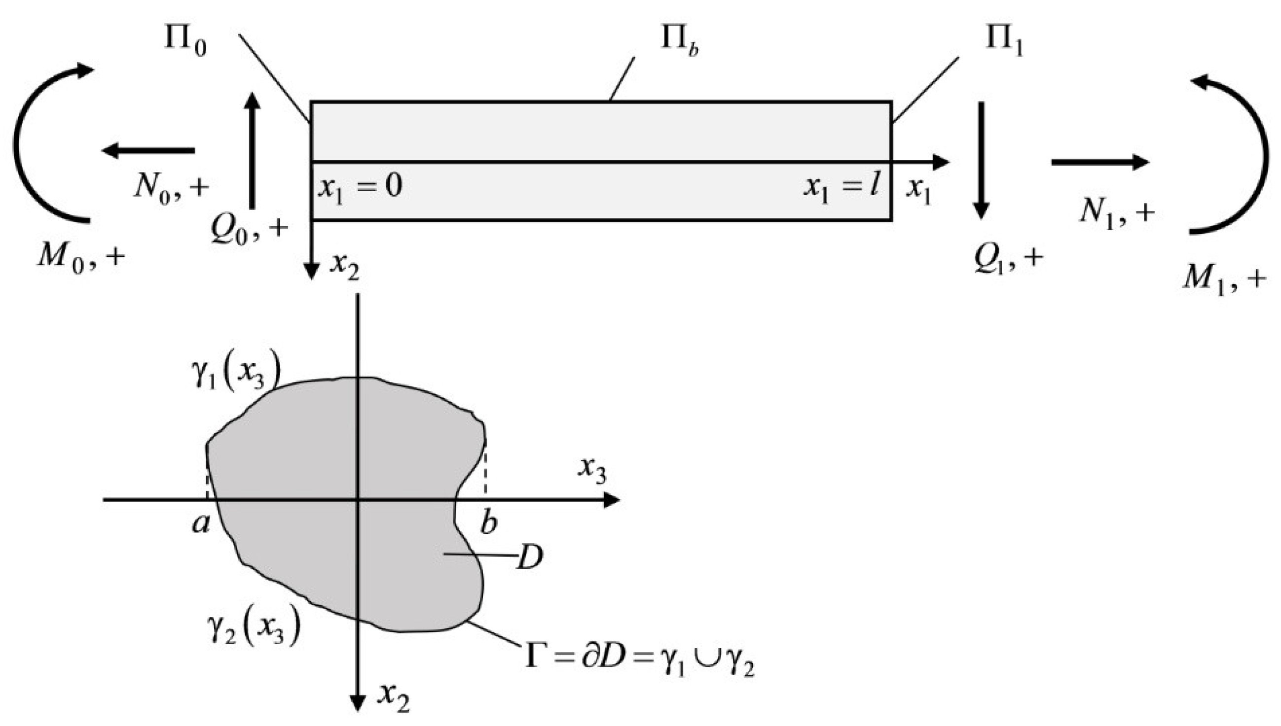
2. Problem Formulation

We consider the unsteady oscillation problem of elastic diffusion Euler–Bernoulli beam in the presence of diffusion flux relaxation. The beam in general formulation is under the action of longitudinal and transverse forces. Also, bending moments are at its ends. The load scheme is presented in Figure 1.

For the mathematical problem formulation, we use the coupled elastic diffusion continuum model in a rectangular Cartesian coordinate system, which has the following form [1,2,3,4,5,6,7,8,9,10,11,12,13,14,15,16,17,18]:

$${\ddot{u}}_i=\frac{\partial {\mathsf{\sigma }}_{ij}}{\partial x_j}+F_i,{\dot{\mathsf{\eta }}}^{\left(q\right)}=-\frac{\partial J_i^{\left(q\right)}}{\partial x_i}+Y^{\left(q\right)}\left(q=\overline{1,N}\right).$$

(1)

where the point denotes a time derivative; ${\mathsf{\sigma }}_{ij}$ and $J_i^{\left(q\right)}$ are the stress tensor components and the diffusion flux vector, respectively. They are defined as follows (the beam material is perfect solid solution):

$${\mathsf{\sigma }}_{ij}=C_{ijkl}\frac{\partial u_k}{\partial x_l}-{\displaystyle \sum _{q=1}^N{\mathsf{\alpha }}_{ij}^{\left(q\right)}{\mathsf{\eta }}^{\left(q\right)}},J_i^{\left(q\right)}+{\mathsf{\tau }}^{\left(q\right)}{\dot{J}}_i^{\left(q\right)}=-D_{ij}^{\left(q\right)}\frac{\partial {\mathsf{\eta }}^{\left(q\right)}}{\partial x_j}+{\mathsf{\Lambda }}_{ijkl}^{\left(q\right)}\frac{{\partial }^2{u}_k}{\partial x_j\partial x_l}\left(q=\overline{1,N}\right).$$

(2)

Here, the dots denote the time derivative. All quantities in (1) and (2) are dimensionless. For them, the following notations are used:

$$\begin{array}{l}{x}_i=\frac{x_i^{\ast }}{l},u_i=\frac{u_i^{\ast }}{l},\mathsf{\tau }=\frac{Ct}{l},C_{ijkl}=\frac{C_{ijkl}^{\ast }}{C_{1111}},C^2=\frac{C_{1111}^{\ast }}{\rho },{\mathsf{\alpha }}_{ij}^{\left(q\right)}=\frac{{\mathsf{\alpha }}_{ij}^{\ast \left(q\right)}}{C_{1111}},\\ {\mathsf{\tau }}_q=\frac{C{\mathsf{\tau }}^{\left(q\right)}}{L},D_{ij}^{\left(q\right)}=\frac{D_{ij}^{\ast \left(q\right)}}{Cl},{\mathsf{\Lambda }}_{ijkl}^{\left(q\right)}=\frac{m^{\left(q\right)}{D}_{ij}^{\ast \left(q\right)}{\mathsf{\alpha }}_{kl}^{\ast \left(q\right)}{n}_0^{\left(q\right)}}{\rho R{T}_{0}Cl},F_i=\frac{\rho l{F}_i^{\ast }}{{С}_{1111}},Y^{\left(q\right)}=\frac{l{Y}^{\ast \left(q\right)}}{C},\end{array}$$

(3)

where $t$ is time; $x_i^{*}$ are rectangular Cartesian coordinates; $\rho$ is the medium density; $u_i^{*}$ are displacement vector components; $C_{ijkl}^{\ast }$ are elastic constant tensor components; $T_0$ is the initial temperature; $D_{ij}^{*\left(q\right)}$ are the self-diffusion coefficients; $R$ is the universal gas constant; $m^{\left(q\right)}$ is the molar mass; ${\mathsf{\eta }}^{\left(q\right)}=n^{\left(q\right)}-n_0^{\left(q\right)}$ is the concentration increment of $q$-th component in the $N$-component medium; $n_0^{\left(q\right)}$ and $n^{(q)}$ are the initial and actual concentrations (mass fractions); ${\mathsf{\alpha }}_{ij}^{*\left(q\right)}$ are coefficients characterizing the medium volumetric changes due to diffusion; $l$ is beam length; $F_i$ and $Y^{\left(q\right)}$ are mechanical and diffusive bulk perturbations; and ${\mathsf{\tau }}^{\left(q\right)}$ is the relaxation time of diffusion perturbations.

The formulation of the problem is completed by the initial and boundary conditions.

Initial conditions:

$${u_i|}_{\mathsf{\tau }=t_0}=u_{i0},{{\dot{u}}_i|}_{\mathsf{\tau }=t_0}=v_{i0},{{\mathsf{\eta }}^{\left(q\right)}|}_{\mathsf{\tau }=t_0}={\mathsf{\eta }}_0^{\left(q\right)}\left(q=\overline{1,N}\right).$$

(4)

Here, $u_{i0}$, $v_{i0}$, ${\mathsf{\eta }}_0^{\left(q\right)}$ are the given functions of spatial coordinates. Further in the paper, we assume that $t_0=0$, $u_{i0}=0$, $v_{i0}=0$, ${\mathsf{\eta }}_0^{\left(q\right)}=0$.

Boundary conditions (domain $G$ is bounded; $n_i$ are components of the outer normal unit vector to $\partial G$, $\partial G={\mathsf{\Pi }}_u\cup {\mathsf{\Pi }}_{\mathsf{\sigma }}={\mathsf{\Pi }}_{\mathsf{\eta }}\cup {\mathsf{\Pi }}_J$):

$${u_i|}_{{\mathsf{\Pi }}_u}=U_i,{{\mathsf{\sigma }}_{ij}{n}_j|}_{{\mathsf{\Pi }}_{\mathsf{\sigma }}}=P_i,{{\mathsf{\eta }}^{\left(q\right)}|}_{{\mathsf{\Pi }}_{\mathsf{\eta }}}=N^{\left(q\right)},{\left(J_i^{\left(q\right)}+{\mathsf{\tau }}_q{\dot{J}}_i^{\left(q\right)}\right)|}_{{\mathsf{\Pi }}_J}=I_i^{\left(q\right)}\left(\mathsf{\tau }>0,q=\overline{1,N}\right).$$

(5)

The quantities on the boundary conditions on right sides are surface kinematic $U_i$, $N^{\left(q\right)}$ and dynamic $P_i$, $I_i^{\left(q\right)}$ perturbations.

To construct the beam bending equations, a transition to the variational formulation of the problem (1)–(5) is used. According to Hamilton’s variational principle, the relations (1)–(5) can be regarded as a condition for the stationarity of a certain functional $H\left(u_i,{\mathsf{\eta }}^{\left(q\right)}\right)$, whose variation is written thus:

$$\begin{array}{l}\delta H={\displaystyle \underset{t_1}{\overset{t_2}{\int }}d\mathsf{\tau }{\displaystyle \underset{G}{\int }\left({\ddot{u}}_i-\frac{\partial {\mathsf{\sigma }}_{ij}}{\partial x_j}-F_i\right)\delta u_{i}dG}}+{\displaystyle \sum _{q=1}^N{\displaystyle \underset{t_1}{\overset{t_2}{\int }}d\mathsf{\tau }{\displaystyle \underset{G}{\int }\left(1+{\mathsf{\tau }}_q\frac{\partial }{\partial \mathsf{\tau }}\right)\left({\dot{\mathsf{\eta }}}^{\left(q\right)}+\frac{\partial J_i^{\left(q\right)}}{\partial x_i}-Y^{\left(q\right)}\right)\delta {\mathsf{\eta }}^{\left(q\right)}dG}}}+\hfill \\ +{\displaystyle \underset{t_1}{\overset{t_2}{\int }}{\displaystyle \underset{{\mathsf{\Pi }}_{\mathsf{\sigma }}}{\iint }\left({\mathsf{\sigma }}_{ij}{n}_j-P_i\right)}}\delta u_{i}dSd\mathsf{\tau }+{\displaystyle \sum _{q=1}^N{\displaystyle \underset{t_1}{\overset{t_2}{\int }}{\displaystyle \underset{{\mathsf{\Pi }}_J}{\iint }\left(J_i^{\left(q\right)}+{\mathsf{\tau }}_q{\dot{J}}_i^{\left(q\right)}-I_i^{\left(q\right)}\right)}}{n}_i\delta {\mathsf{\eta }}^{\left(q\right)}dSd\mathsf{\tau }}.\hfill \end{array}$$

(6)

Further, we will assume that

• The axis $O{x}_3$ is the central axis of the cross section. In this case,

  $${\displaystyle \underset{D}{\iint }{x}_{2}d{x}_{2}d{x}_3}=0.$$

  (7)
• The side surface ${\mathsf{\Pi }}_b$ is free from mechanical loads, i.e.,

  $${{\mathsf{\sigma }}_{ij}{n}_j|}_{{\mathsf{\Pi }}_b}=0.$$

  (8)
• We also assume that there is no mass transfer through the side surface,

  $${\left(J_i^{\left(q\right)}+{\mathsf{\tau }}_q{\dot{J}}_i^{\left(q\right)}\right)|}_{{\mathsf{\Pi }}_b}=0.$$

  (9)
• The beam material is a homogeneous ortotropic continuum.
  The bending of beam is considered in plane $x_{1}O{x}_2$. Then $u_k=u_k\left(x_1,x_2,\mathsf{\tau }\right),$ $k=1,2$; $u_3=0$; ${\epsilon }_{i3}=0$. Mass transfer occurs also in the plane $x_{1}O{x}_2$, i.e., η^(q) = η^(q)(x₁,x₂,τ).
• Transverse deflections are considered small. Then, the linearization of the unknown quantities with respect to the variable $x_2$ will have the following form:

  $$\begin{array}{l}{u}_1\left(x_1,x_2,\mathsf{\tau }\right)=u\left(x_1,\mathsf{\tau }\right)-x_2\chi \left(x_1,\mathsf{\tau }\right),u_2\left(x_1,x_2,\mathsf{\tau }\right)=v\left(x_1,\mathsf{\tau }\right)+x_2\mathsf{\psi }\left(x_1,\mathsf{\tau }\right),\\ {\mathsf{\eta }}^{\left(q\right)}\left(x_1,x_2,\mathsf{\tau }\right)=N_q\left(x_1,\mathsf{\tau }\right)+x_2{H}_q\left(x_1,\mathsf{\tau }\right).\end{array}$$

  (10)
• The cross sections after deformation remain normal to the neutral line of the beam (Euler–Bernoulli ’s beam theory). Also, we assume that there are no deformations along the $O{x}_2$ axis [24,25].

  $${\epsilon }_{22}=\frac{\partial u_2}{\partial x_2}=\mathsf{\psi }=0\Rightarrow \mathsf{\psi }=0,\chi \left(x_1,\mathsf{\tau }\right)=v^{\prime }\left(x_1,\mathsf{\tau }\right).$$

Then, Equation (10) will take the following form:

$$u_1=u-x_2{v}^{\prime },u_2=v,u_3=0,u=u\left(x_1,\mathsf{\tau }\right),v=v\left(x_1,\mathsf{\tau }\right).$$

(11)

Here, the prime denotes the derivative with respect to the variable $x_1$.

From (8) and (9), it follows that,

$${{\mathsf{\sigma }}_{22}{n}_2|}_{{\mathsf{\Pi }}_b}={{\mathsf{\sigma }}_{22}{n}_2|}_{\mathsf{\Gamma }}={{\mathsf{\sigma }}_{22}|}_{{\gamma }_2\left(x_3\right)}^{{\gamma }_1\left(x_3\right)}=0;$$

(12)

$${\displaystyle \underset{G}{\int }\frac{\partial {\mathsf{\sigma }}_{22}}{\partial x_2}dG}={\displaystyle \underset{0}{\overset{1}{\int }}d{x}_1}{\displaystyle \underset{D}{\iint }\frac{\partial {\mathsf{\sigma }}_{22}}{\partial x_2}d{x}_{2}d{x}_3}={\displaystyle \underset{0}{\overset{1}{\int }}d{x}_1}{\displaystyle \underset{a}{\overset{b}{\int }}{\displaystyle \underset{{\gamma }_2\left(x_3\right)}{\overset{{\gamma }_1\left(x_3\right)}{\int }}\frac{\partial {\mathsf{\sigma }}_{22}}{\partial x_2}d{x}_{2}d{x}_3}}={\displaystyle \underset{0}{\overset{1}{\int }}d{x}_1}{\displaystyle \underset{a}{\overset{b}{\int }}{{\mathsf{\sigma }}_{22}|}_{{\gamma }_2\left(x_3\right)}^{{\gamma }_1\left(x_3\right)}d{x}_3}=0.$$

(13)

The components of the stress tensor and the diffusion flow vector will have the following form:

$$\begin{array}{l}{\mathsf{\sigma }}_{11}=C_{11}\frac{\partial u_1}{\partial x_1}+C_{12}\frac{\partial u_2}{\partial x_2}-{\displaystyle \sum _{q=1}^N{\mathsf{\alpha }}_1^{\left(q\right)}{\mathsf{\eta }}^{\left(q\right)}}=\left(u^{\prime }-x_2{v}^{″}\right)-{\displaystyle \sum _{q=1}^N{\mathsf{\alpha }}_1^{\left(q\right)}\left(N_q+x_2{H}_q\right)},{\mathsf{\sigma }}_{12}=C_{66}\left(\frac{\partial u_1}{\partial x_2}+\frac{\partial u_2}{\partial x_1}\right)=0,\hfill \\ {\mathsf{\sigma }}_{22}=C_{12}\frac{\partial u_1}{\partial x_1}+C_{22}\frac{\partial u_2}{\partial x_2}-{\displaystyle \sum _{q=1}^N{\mathsf{\alpha }}_2^{\left(q\right)}{\mathsf{\eta }}^{\left(q\right)}}=C_{12}\left(u^{\prime }-x_2{v}^{″}\right)-{\displaystyle \sum _{q=1}^N{\mathsf{\alpha }}_2^{\left(q\right)}\left(N_q+x_2{H}_q\right)},\hfill \\ J_1^{\left(q\right)}+{\mathsf{\tau }}_q{\dot{J}}_1^{\left(q\right)}=-D_1^{\left(q\right)}\frac{\partial {\mathsf{\eta }}^{\left(q\right)}}{\partial x_1}+{\mathsf{\Lambda }}_{11}^{\left(q\right)}\frac{{\partial }^2{u}_1}{\partial x_1^2}+{\mathsf{\Lambda }}_{12}^{\left(q\right)}\frac{{\partial }^2{u}_2}{\partial x_1\partial x_2}=-D_1^{\left(q\right)}\left({N^{\prime }}_q+x_2{H^{\prime }}_q\right)+{\mathsf{\Lambda }}_{11}^{\left(q\right)}\left(u^{″}-x_2{v}^{‴}\right),\hfill \\ J_2^{\left(q\right)}+{\mathsf{\tau }}_q{\dot{J}}_2^{\left(q\right)}=-D_2^{\left(q\right)}\frac{\partial {\mathsf{\eta }}^{\left(q\right)}}{\partial x_2}+{\mathsf{\Lambda }}_{22}^{\left(q\right)}\frac{{\partial }^2{u}_2}{\partial x_2^2}+{\mathsf{\Lambda }}_{21}^{\left(q\right)}\frac{{\partial }^2{u}_1}{\partial x_1\partial x_2}=-D_2^{\left(q\right)}{H}_q-{\mathsf{\Lambda }}_{21}^{\left(q\right)}{v}^{″}\left(q=\overline{1,N}\right),\hfill \end{array}$$

(14)

where

$$\begin{array}{l}{C}_{11}=C_{1111},C_{12}=C_{1122},C_{22}=C_{2222},C_{66}=C_{1212},{\mathsf{\alpha }}_1^{\left(q\right)}={\mathsf{\alpha }}_{11}^{\left(q\right)},{\mathsf{\alpha }}_2^{\left(q\right)}={\mathsf{\alpha }}_{22}^{\left(q\right)},\\ D_1^{\left(q\right)}=D_{11}^{\left(q\right)},D_2^{\left(q\right)}=D_{22}^{\left(q\right)},{\mathsf{\Lambda }}_{11}^{\left(q\right)}={\mathsf{\Lambda }}_{1111}^{\left(q\right)},{\mathsf{\Lambda }}_{12}^{\left(q\right)}={\mathsf{\Lambda }}_{1122}^{\left(q\right)},{\mathsf{\Lambda }}_{21}^{\left(q\right)}={\mathsf{\Lambda }}_{2211}^{\left(q\right)},{\mathsf{\Lambda }}_{22}^{\left(q\right)}={\mathsf{\Lambda }}_{2222}^{\left(q\right)}.\end{array}$$

Substituting the relations (7), (10)–(14) into (6), we obtain the following:

$$\begin{array}{l}\delta H={\displaystyle \underset{t_1}{\overset{t_2}{\int }}d\mathsf{\tau }{\displaystyle \underset{0}{\overset{1}{\int }}\left[F\left(\ddot{u}-u^{″}+{\displaystyle \sum _{q=1}^N{\mathsf{\alpha }}_1^{\left(q\right)}{N}^{\prime }}\right)-n\right]\delta ud{x}_1}}-{\displaystyle \underset{t_1}{\overset{t_2}{\int }}d\mathsf{\tau }{\displaystyle \underset{0}{\overset{1}{\int }}\left[J_3\left({\ddot{v}}^{″}-v^{IV}-{\displaystyle \sum _{q=1}^N{\mathsf{\alpha }}_1^{\left(q\right)}{H^{″}}_q}\right)+m^{\prime }\right]\delta vd{x}_1}}+\\ +{\displaystyle \underset{t_1}{\overset{t_2}{\int }}d\mathsf{\tau }{\displaystyle \underset{0}{\overset{1}{\int }}\left(F\ddot{v}-q\right)\delta vd{x}_1}}+{\displaystyle \sum _{q=1}^N{\displaystyle \underset{t_1}{\overset{t_2}{\int }}d\mathsf{\tau }}{\displaystyle \underset{0}{\overset{1}{\int }}\left[F\left({\dot{N}}_q+{\mathsf{\tau }}^{\left(q\right)}{\ddot{N}}_q-D_1^{\left(q\right)}{N^{″}}_q+{\mathsf{\Lambda }}_{11}^{\left(q\right)}{u}^{‴}\right)-y^{\left(q\right)}\right]\delta N_{q}d{x}_1}}+\\ +{\displaystyle \sum _{q=1}^N{\displaystyle \underset{t_1}{\overset{t_2}{\int }}d\mathsf{\tau }}{\displaystyle \underset{0}{\overset{1}{\int }}\left[J_3\left({\dot{H}}_q+{\mathsf{\tau }}^{\left(q\right)}{\ddot{H}}_q-D_1^{\left(q\right)}{H^{″}}_q-{\mathsf{\Lambda }}_{11}^{\left(q\right)}{v}^{IV}\right)-z^{\left(q\right)}\right]\delta H_{q}d{x}_1}}+\\ +{\displaystyle \underset{t_1}{\overset{t_2}{\int }}{\left[J_3\left({\ddot{v}}^{\prime }-v^{‴}-{\displaystyle \sum _{q=1}^N{\mathsf{\alpha }}_1^{\left(q\right)}{H^{\prime }}_q}\right)+m\right]\delta v|}_{x_1=0}^{x_1=1}d\mathsf{\tau }}+\\ +{\displaystyle \underset{t_1}{\overset{t_2}{\int }}{\left\{\left[F\left(u^{\prime }-{\displaystyle \sum _{q=1}^N{\mathsf{\alpha }}_1^{\left(q\right)}{N}_q}\right)-N\right]\delta u+\left[J_3\left(v^{″}+{\displaystyle \sum _{q=1}^N{\mathsf{\alpha }}_1^{\left(q\right)}{H}_q}\right)+M\right]\delta v^{\prime }-Q\delta v\right\}|}_{x_1=0}^{x_1=1}}d\mathsf{\tau }+\\ +{\displaystyle \sum _{q=1}^N{\displaystyle \underset{t_1}{\overset{t_2}{\int }}{\left\{\left[F\left(-D_1^{\left(q\right)}{N^{\prime }}_q+{\mathsf{\Lambda }}_{11}^{\left(q\right)}{u}^{″}\right)-{\mathsf{\Gamma }}^{\left(q\right)}\right]\delta N_q-\left[J_3\left(D_1^{\left(q\right)}{H^{\prime }}_q+{\mathsf{\Lambda }}_{11}^{\left(q\right)}{v}^{‴}\right)+{\mathsf{\Omega }}^{\left(q\right)}\right]\delta H_q\right\}|}_{x_1=0}^{x_1=1}d\mathsf{\tau }}}.\end{array}$$

We introduce the following notation:

• ${\displaystyle \underset{D}{\iint }d{x}_{2}d{x}_3}=F$ is the cross-sectional area,
• ${\displaystyle \underset{D}{\iint }{x}_2^{2}d{x}_{2}d{x}_3}=J_3$ is moment of inertia of the beam section relative to the axis $O{x}_3$,
• ${\displaystyle \underset{D}{\iint }{F}_{1}d{x}_{2}d{x}_3}=n$ is the linearly distributed axial load,
• ${\displaystyle \underset{D}{\iint }{F}_1{x}_{2}d{x}_{2}d{x}_3}=m$ is the linearly distributed moment,
• ${\displaystyle \underset{D}{\iint }{F}_{2}d{x}_{2}d{x}_3}=q$ is the linearly distributed transverse load,
• ${\displaystyle \underset{D}{\iint }\left(Y^{\left(q\right)}+{\mathsf{\tau }}^{\left(q\right)}{\dot{Y}}^{\left(q\right)}\right)d{x}_{2}d{x}_3}=y^{\left(q\right)}$ is the linear density of bulk mass transfer sources,

  $$\begin{gathered} {\displaystyle \underset{D}{\iint }\left(Y^{\left(q\right)}+{\mathsf{\tau }}^{\left(q\right)}{\dot{Y}}^{\left(q\right)}\right)x_{2}d{x}_{2}d{x}_3}=z^{\left(q\right)}, \\ N\left(x_1\right)={\displaystyle \underset{D}{\iint }{P}_1\left(x_1,x_2,x_3,\mathsf{\tau }\right)d{x}_{2}d{x}_3},M\left(x_1\right)={\displaystyle \underset{D}{\iint }{P}_1\left(x_1,x_2,x_3,\mathsf{\tau }\right)x_{2}d{x}_{2}d{x}_3},Q\left(x_1\right)={\displaystyle \underset{D}{\iint }{P}_2\left(x_1,x_2,x_3,\mathsf{\tau }\right)d{x}_{2}d{x}_3}, \\ {\mathsf{\Gamma }}^{\left(q\right)}\left(x_1\right)={\displaystyle \underset{D}{\iint }{I}_1^{\left(q\right)}\left(x_1,x_2,x_3,\mathsf{\tau }\right)d{x}_{2}d{x}_3},{\mathsf{\Omega }}^{\left(q\right)}\left(x_1\right)={\displaystyle \underset{D}{\iint }{x}_2{I}_1^{\left(q\right)}\left(x_1,x_2,x_3,\mathsf{\tau }\right)d{x}_{2}d{x}_3}. \end{gathered}$$

Thus, the following boundary-value problems are the necessary conditions for the stationarity of the Hamilton functional considering (7)–(11):

$$\ddot{u}=u^{″}-{\displaystyle \sum _{q=1}^N{\mathsf{\alpha }}_1^{\left(q\right)}{N^{\prime }}_q}+\frac{n}{F},{\dot{N}}_q+{\mathsf{\tau }}_q{\ddot{N}}_q=D_1^{\left(q\right)}{N^{″}}_q-{\mathsf{\Lambda }}_{11}^{\left(q\right)}{u}^{‴}+\frac{y^{\left(q\right)}}{F};$$

(15)

$${\left(u^{\prime }-{\displaystyle \sum _{q=1}^N{\mathsf{\alpha }}_1^{\left(q\right)}{N}_q}\right)|}_{x_1=0}=\frac{N_0}{F},{\left(u^{\prime }-{\displaystyle \sum _{q=1}^N{\mathsf{\alpha }}_1^{\left(q\right)}{N}_q}\right)|}_{x_1=1}=\frac{N_1}{F};$$

(16)

$${\left(-D_1^{\left(q\right)}{N^{\prime }}_q+{\mathsf{\Lambda }}_{11}^{\left(q\right)}{u}^{″}\right)|}_{x_1=0}=\frac{{\mathsf{\Gamma }}_0^{\left(q\right)}}{F},{\left(-D_1^{\left(q\right)}{N^{\prime }}_q+{\mathsf{\Lambda }}_{11}^{\left(q\right)}{u}^{″}\right)|}_{x_1=1}=\frac{{\mathsf{\Gamma }}_1^{\left(q\right)}}{F};$$

(17)

$$\begin{array}{l}{\ddot{v}}^{″}-\frac{F}{J_3}\ddot{v}=v^{IV}+{\displaystyle \sum _{j=1}^N{\mathsf{\alpha }}_1^{\left(q\right)}{H^{″}}_j}-\frac{q}{J_3}-\frac{m^{\prime }}{J_3},\\ {\dot{H}}_q+{\mathsf{\tau }}_q{\ddot{H}}_q=D_1^{\left(q\right)}{H^{″}}_q+{\mathsf{\Lambda }}_{11}^{\left(q\right)}{v}^{IV}+\frac{z^{\left(q\right)}}{J_3};\end{array}$$

(18)

$${\left(v^{″}+{\displaystyle \sum _{j=1}^N{\mathsf{\alpha }}_1^{\left(q\right)}{H}_j}\right)|}_{x_1=0}=-\frac{M_0}{J_3},{\left(v^{″}+{\displaystyle \sum _{j=1}^N{\mathsf{\alpha }}_1^{\left(q\right)}{H}_j}\right)|}_{x_1=1}=-\frac{M_1}{J_3};$$

(19)

$${\left(v^{‴}+{\displaystyle \sum _{j=1}^N{\mathsf{\alpha }}_1^{\left(q\right)}{H^{\prime }}_j}-\ddot{v^{\prime }}\right)|}_{x_1=0}=\frac{Q_0+{m|}_{x_1=0}}{J_3},{\left(v^{‴}+{\displaystyle \sum _{j=1}^N{\mathsf{\alpha }}_1^{\left(q\right)}{H^{\prime }}_j}-\ddot{v^{\prime }}\right)|}_{x_1=1}=\frac{Q_1+{m|}_{x_1=1}}{J_3};$$

(20)

$${\left(D_1^{\left(q\right)}{H^{\prime }}_q+{\mathsf{\Lambda }}_{11}^{\left(q\right)}{v}^{‴}\right)|}_{x_1=0}=-\frac{{\mathsf{\Omega }}_0^{\left(q\right)}}{J_3},{\left(D_1^{\left(q\right)}{H^{\prime }}_q+{\mathsf{\Lambda }}_{11}^{\left(q\right)}{v}^{‴}\right)|}_{x_1=1}=-\frac{{\mathsf{\Omega }}_1^{\left(q\right)}}{J_3},$$

(21)

where

$$\begin{array}{l}{N}_0=N\left(0\right),N_1=N\left(1\right),M_0=M\left(0\right),M_1=M\left(1\right),Q_0=Q\left(0\right),Q_1=Q\left(1\right),\\ {\mathsf{\Gamma }}_0^{\left(q\right)}={\mathsf{\Gamma }}^{\left(q\right)}\left(0\right),{\mathsf{\Gamma }}_1^{\left(q\right)}={\mathsf{\Gamma }}^{\left(q\right)}\left(1\right),{\mathsf{\Omega }}_0^{\left(q\right)}={\mathsf{\Omega }}^{\left(q\right)}\left(0\right),{\mathsf{\Omega }}_1^{\left(q\right)}={\mathsf{\Omega }}^{\left(q\right)}\left(1\right).\end{array}$$

In accordance with the variational principle of Lagrange, the boundary conditions (15)–(21) combined with the kinematic boundary conditions are as follows:

$${u|}_{x_1=0}=U_0,{u|}_{x_1=1}=U_1;$$

(22)

$${N_q|}_{x_1=0}=N_{q0},{N_q|}_{x_1=1}=N_{q1};$$

(23)

$${v|}_{x_1=0}=V_0,{v|}_{x_1=1}=V_1;$$

(24)

$${v^{\prime }|}_{x_1=0}={V^{\prime }}_0,{v^{\prime }|}_{x_1=1}={V^{\prime }}_1;$$

(25)

$${H_q|}_{x_1=0}=H_{q0},{H_q|}_{x_1=1}=H_{q1};$$

(26)

$${{H^{\prime }}_q|}_{x_1=0}={H^{\prime }}_{q0},{{H^{\prime }}_q|}_{x_1=1}={H^{\prime }}_{q1}.$$

(27)

Problems (15), (16), and (23) as well as (15), (17), and (22) are equivalent to one-dimensional problems of elastic diffusion for a layer. Their solutions are constructed using Laplace transform and decomposition into trigonometric Fourier series [26,27,28]. The papers [29,30] also considered problems with other combinations of boundary conditions that are solved by the method of equivalent boundary conditions.

Thus, the object of further consideration in this article will be initial boundary value problems for Equation (18) with a combination of boundary conditions (19), (20), and (24)–(27). Initial conditions will be assumed to be zero.

3. Method of Solution

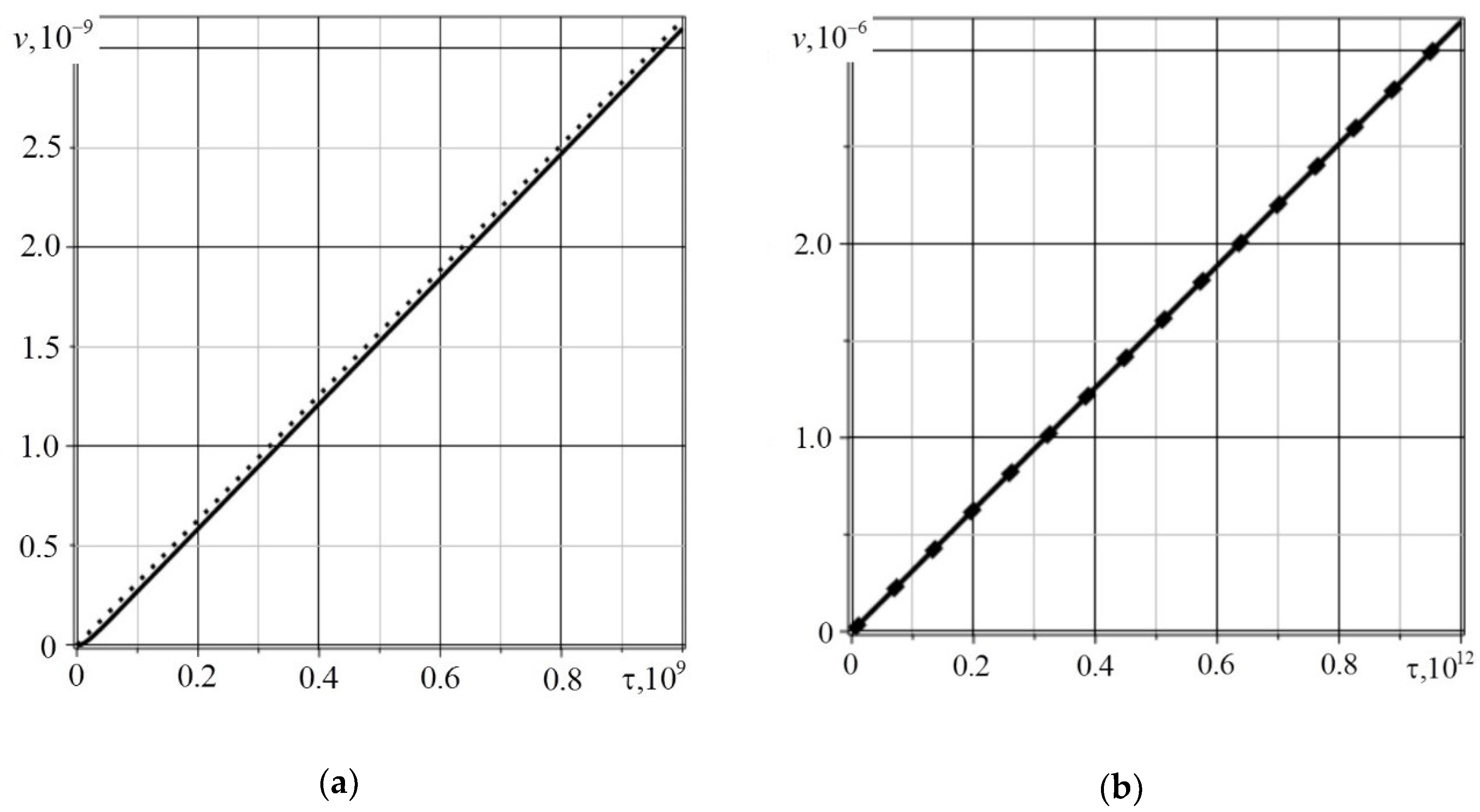
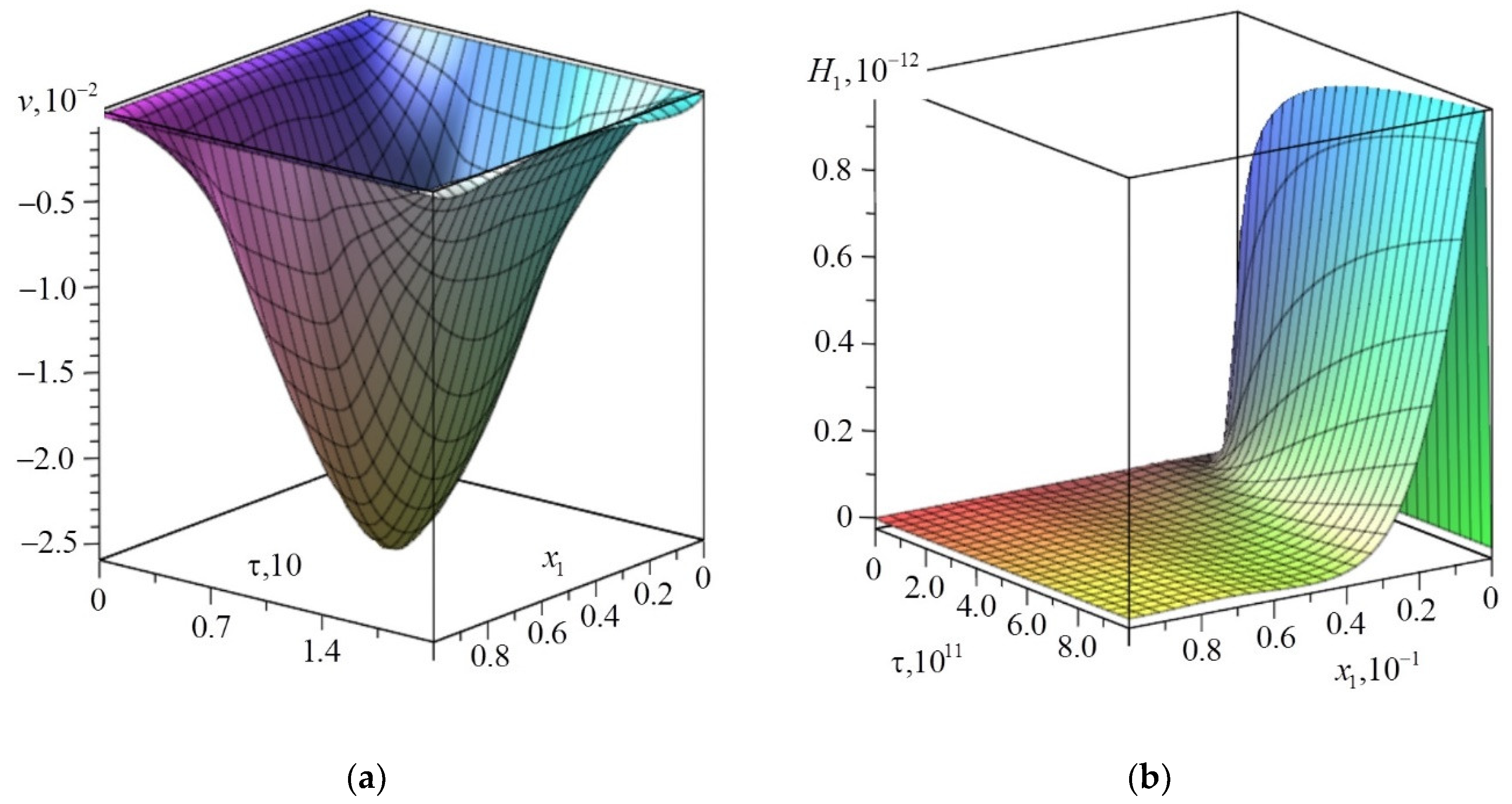
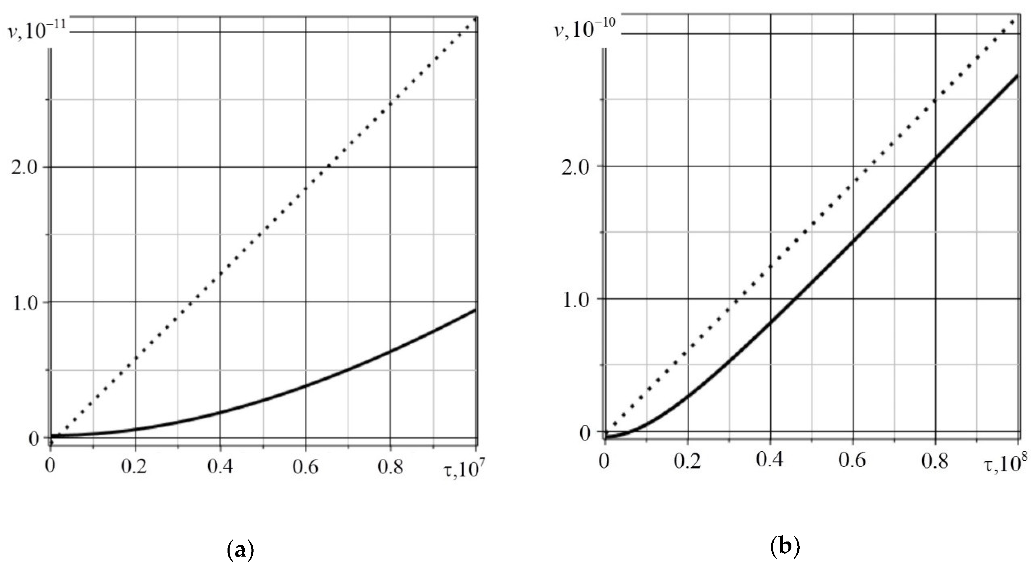
We consider the problems (18), (19), (24), (26). The solutions of the problem are represented in the form ($q=\overline{1,N+1}$):

$$\begin{array}{l}v\left(x,\mathsf{\tau }\right)={\displaystyle \sum _{k=1}^{N+2}{\displaystyle \underset{0}{\overset{\mathsf{\tau }}{\int }}\left[G_{1k}\left(x,\mathsf{\tau }-t\right)f_{k1}\left(t\right)+G_{1k}\left(1-x,\mathsf{\tau }-t\right)f_{k2}\left(t\right)\right]dt}}+{\displaystyle \sum _{k=1}^{N+1}{\displaystyle \underset{0}{\overset{\mathsf{\tau }}{\int }}{\displaystyle \underset{0}{\overset{1}{\int }}{\tilde{G}}_{1k}\left(x,\xi ,\mathsf{\tau }-t\right)F_k\left(\xi ,t\right)d\xi }dt}},\\ H_q\left(x,\mathsf{\tau }\right)={\displaystyle \sum _{k=1}^{N+2}{\displaystyle \underset{0}{\overset{\mathsf{\tau }}{\int }}\left[G_{q+1,k}\left(x,\mathsf{\tau }-t\right)f_{k1}\left(t\right)+G_{q+1,k}\left(1-x,\mathsf{\tau }-t\right)f_{k2}\left(t\right)\right]dt}}+\\ +{\displaystyle \sum _{k=1}^{N+1}{\displaystyle \underset{0}{\overset{\mathsf{\tau }}{\int }}{\displaystyle \underset{0}{\overset{1}{\int }}{\tilde{G}}_{q+1,k}\left(x,\xi ,\mathsf{\tau }-t\right)F_k\left(\xi ,t\right)d\xi }dt}}.\end{array}$$

(28)

Here, $x=x_1$; $G_{mk}$ and ${\tilde{G}}_{mk}$ are surface and bulk Green’s functions; $F_1\left(x,\mathsf{\tau }\right)=\left(q+m^{\prime }\right)/J_3$ and $F_{q+1}\left(x,\mathsf{\tau }\right)=z^{\left(q\right)}/J_3$ are body forces entering into Equation (18); and $f_{kl}\left(t\right)$ are surface disturbances that have the following form:

$$\begin{array}{l}{f}_{11}\left(\mathsf{\tau }\right)=-\frac{M_0\left(\mathsf{\tau }\right)}{J_3},f_{12}\left(\mathsf{\tau }\right)=-\frac{M_1\left(\mathsf{\tau }\right)}{J_3},\\ f_{21}\left(\mathsf{\tau }\right)=V_0,f_{22}\left(\mathsf{\tau }\right)=V_1,f_{q+2,1}\left(\mathsf{\tau }\right)=H_{q0}\left(\mathsf{\tau }\right),f_{q+2,2}\left(\mathsf{\tau }\right)=H_{q1}\left(\mathsf{\tau }\right).\end{array}$$

The surface Green’s functions $G_{mk}$ satisfy

$$\begin{array}{l}{{\ddot{G}}^{″}}_{1k}-\frac{F}{J_3}{\ddot{G}}_{1k}=G_{1k}^{IV}+{\displaystyle \sum _{j=1}^N{\mathsf{\alpha }}_1^{\left(j\right)}{G^{″}}_{j+1,k}},\\ {\dot{G}}_{q+1,k}+{\mathsf{\tau }}_q{\ddot{G}}_{q+1,k}=D_1^{\left(q\right)}{G^{″}}_{q+1,k}+{\mathsf{\Lambda }}_{11}^{\left(q\right)}{G}_{1k}^{IV},\end{array}$$

(29)

$$\begin{array}{l}{\left({G^{″}}_{1k}+{\displaystyle \sum _{j=1}^N{\mathsf{\alpha }}_1^{\left(j\right)}{G}_{j+1,k}}\right)|}_{x_1=0}={\delta }_{1k}\delta \left(\mathsf{\tau }\right),{\left({G^{″}}_{1k}+{\displaystyle \sum _{j=1}^N{\mathsf{\alpha }}_1^{\left(j\right)}{G}_{j+1,k}}\right)|}_{x_1=1}=0,\\ {G_{1k}|}_{x_1=0}={\delta }_{2k}\delta \left(\mathsf{\tau }\right),{G_{1k}|}_{x_1=1}=0,{G_{q+1,k}|}_{x_1=0}={\delta }_{q+2,k}\delta \left(\mathsf{\tau }\right),{G_{q+1,k}|}_{x_1=1}=0.\end{array}$$

(30)

The bulk Green’s functions ${\tilde{G}}_{mk}$ satisfy

$$\begin{array}{l}{\ddot{\tilde{G}}}_{1k}^{″}-\frac{F}{J_3}{\ddot{\tilde{G}}}_{1k}={\tilde{G}}_{1k}^{IV}+{\displaystyle \sum _{j=1}^N{\mathsf{\alpha }}_1^{\left(j\right)}{\widetilde{G^{″}}}_{j+1,k}}-{\delta }_{1k}\delta \left(x-\xi \right)\delta \left(\mathsf{\tau }\right),\\ {\dot{\tilde{G}}}_{q+1,k}+{\mathsf{\tau }}_q{\ddot{\tilde{G}}}_{q+1,k}=D_1^{\left(q\right)}{\widetilde{G^{″}}}_{q+1,k}+{\mathsf{\Lambda }}_{11}^{\left(q\right)}{\tilde{G}}_{1k}^{IV}+{\delta }_{q+1,k}\delta \left(x-\xi \right)\delta \left(\mathsf{\tau }\right),\end{array}$$

and homogeneous boundary conditions corresponding to (30).

We consider the problem of finding the surface Green’s functions $G_{mk}$. Applying the Laplace transformation with respect to time to (29) and (30), we get the following ($s$ is the Laplace transform parameter):

$$\begin{gathered} \begin{array}{l}{s}^2{G}_{1k}^{L^{″}}\left(x,s\right)-\frac{F}{J_3}{s}^2{G}_{1k}^L\left(x,s\right)={\left[G_{1k}^{IV}\left(x,s\right)\right]}^L+{\displaystyle \sum _{j=1}^N{\mathsf{\alpha }}_1^{\left(j\right)}{G}_{j+1,k}^{L^{″}}\left(x,s\right)},\\ \left(s+{\mathsf{\tau }}_q{s}^2\right)G_{q+1,k}^L\left(x,s\right)=D_1^{\left(q\right)}{G}_{q+1,k}^{L^{″}}\left(x,s\right)+{\mathsf{\Lambda }}_{11}^{\left(q\right)}{\left[G_{1k}^{IV}\left(x,s\right)\right]}^L,\end{array} \\ \begin{array}{l}{\left(G_{1k}^{L^{″}}+{\displaystyle \sum _{j=1}^N{\mathsf{\alpha }}_j{G}_{j+1,k}^L}\right)|}_{x_1=0}={\delta }_{1k},{\left({G^{″}}_{1k}^L+{\displaystyle \sum _{j=1}^N{\mathsf{\alpha }}_j{G}_{j+1,k}^L}\right)|}_{x_1=1}=0,\\ {G_{1k}^L|}_{x_1=0}={\delta }_{2k},{G_{1k}^L|}_{x_1=1}=0,{G_{q+1,k}^L|}_{x_1=0}={\delta }_{q+1,k},{G_{q+1,k}^L|}_{x_1=1}=0.\end{array} \end{gathered}$$

Next, we multiply each equation by $\sin {\lambda }_{n}x$ and integrate in the interval $\left[0,1\right]$. The result is as follows:

$$\begin{array}{l}{k}_1\left({\lambda }_n,s\right)G_{1k}^{Ls}\left({\lambda }_n,s\right)-{\lambda }_n^2{\displaystyle \sum _{j=1}^N{\mathsf{\alpha }}_1^{\left(j\right)}{G}_{j+1,k}^{Ls}}\left({\lambda }_n,s\right)=F_{1k}\left({\lambda }_n\right),\\ -{\lambda }_n^4{\mathsf{\Lambda }}_{11}^{\left(q\right)}{G}_{1k}^{Ls}\left({\lambda }_n,s\right)+k_{q+1}\left({\lambda }_n,s\right)G_{q+1,k}^{Ls}\left({\lambda }_n,s\right)=F_{q+1,k}\left({\lambda }_n\right),\end{array}$$

(31)

where

$$\begin{array}{l}{k}_1\left({\lambda }_n,s\right)=\left({\lambda }_n^2+\frac{F}{J_3}\right)s^2+{\lambda }_n^4,F_{q+1,k}\left({\lambda }_n\right)=2{\lambda }_n\left({\mathsf{\Lambda }}_{11}^{\left(q\right)}{\delta }_{1k}-{\mathsf{\Lambda }}_{11}^{\left(q\right)}{\lambda }_n^2{\delta }_{2k}+D_1^{\left(q\right)}{\delta }_{q+2,k}-{\mathsf{\Lambda }}_{11}^{\left(q\right)}{\displaystyle \sum _{j=1}^N{\mathsf{\alpha }}_1^{\left(j\right)}{\delta }_{j+2,k}}\right),\\ k_{q+1}\left({\lambda }_n,s\right)=s+{\mathsf{\tau }}_q{s}^2+D_1^{\left(q\right)}{\lambda }_n^2,F_{1k}\left({\lambda }_n\right)=-2{\lambda }_n{\delta }_{1k}+2{\lambda }_n\left(s^2+{\lambda }_n^2\right){\delta }_{2k},\\ G_{mk}^L\left(x,s\right)={\displaystyle \sum _{n=1}^{\infty }{G}_{mk}^{Ls}\left({\lambda }_n,s\right)\sin {\lambda }_{n}x},G_{mk}^{Ls}\left({\lambda }_n,s\right)=2{\displaystyle \underset{0}{\overset{1}{\int }}{G}_{mk}^L\left(x,s\right)\sin {\lambda }_{n}xdx},{\lambda }_n=\pi n.\end{array}$$

The solution of system (31) has the following form:

$$\begin{array}{l}{G}_{1k}^{Ls}\left({\lambda }_n,s\right)=\frac{P_{1k}\left({\lambda }_n,s\right)}{P\left({\lambda }_n,s\right)},G_{q+1,1}^{Ls}\left({\lambda }_n,s\right)=\frac{2{\lambda }_n{\mathsf{\Lambda }}_{11}^{\left(q\right)}}{k_{q+1}\left({\lambda }_n,s\right)}+\frac{P_{q+1,1}\left({\lambda }_n,s\right)}{Q_q\left({\lambda }_n,s\right)},\hfill \\ G_{q+1,2}^{Ls}\left({\lambda }_n,s\right)=-\frac{2{\mathsf{\Lambda }}_{11}^{\left(q\right)}{\lambda }_n^3}{k_{q+1}\left({\lambda }_n,s\right)}+\frac{P_{q+1,2}\left({\lambda }_n,s\right)}{Q_q\left({\lambda }_n,s\right)},\hfill \\ G_{q+1,p+2}^{Ls}\left({\lambda }_n,s\right)=\frac{2{\lambda }_n\left(D_1^{\left(q\right)}{\delta }_{qp}-{\mathsf{\Lambda }}_{11}^{\left(q\right)}{\mathsf{\alpha }}_p\right)}{k_{q+1}\left({\lambda }_n,s\right)}+\frac{P_{q+1,p+2}\left({\lambda }_n,s\right)}{Q_q\left({\lambda }_n,s\right)}\left(q,p=\overline{1,N},k=\overline{1,N+1}\right).\hfill \end{array}$$

(32)

Here,

$$\begin{gathered} P\left({\lambda }_n,s\right)=k_1\left({\lambda }_n,s\right)\mathsf{\Pi }\left({\lambda }_n,s\right)-{\lambda }_n^6{\displaystyle \sum _{j=1}^N{\mathsf{\Lambda }}_{11}^{\left(j\right)}{\mathsf{\alpha }}_1^{\left(j\right)}{\mathsf{\Pi }}_j}\left({\lambda }_n,s\right),Q_q\left({\lambda }_n,s\right)=k_{q+1}\left({\lambda }_n,s\right)P\left({\lambda }_n,s\right), \\ \begin{array}{l}{P}_{11}\left({\lambda }_n,s\right)=-2{\lambda }_n\left[\mathsf{\Pi }\left({\lambda }_n,s\right)-{\lambda }_n^2{\displaystyle \sum _{j=1}^N{\mathsf{\alpha }}_1^{\left(j\right)}{\mathsf{\Lambda }}_{11}^{\left(j\right)}{\mathsf{\Pi }}_j\left({\lambda }_n,s\right)}\right],\\ P_{12}\left({\lambda }_n,s\right)=2{\lambda }_n\left[\left(s^2+{\lambda }_n^2\right)\mathsf{\Pi }\left({\lambda }_n,s\right)-{\lambda }_n^4{\displaystyle \sum _{j=1}^N{\mathsf{\alpha }}_1^{\left(j\right)}{\mathsf{\Lambda }}_{11}^{\left(j\right)}{\mathsf{\Pi }}_j\left({\lambda }_n,s\right)}\right],\\ P_{1,q+2}\left({\lambda }_n,s\right)=2{\mathsf{\alpha }}_1^{\left(q\right)}{\lambda }_n^3\left[D_1^{\left(q\right)}{\mathsf{\Pi }}_q\left({\lambda }_n,s\right)-{\displaystyle \sum _{j=1}^N{\mathsf{\alpha }}_1^{\left(j\right)}{\mathsf{\Lambda }}_{11}^{\left(j\right)}{\mathsf{\Pi }}_j\left({\lambda }_n,s\right)}\right],\end{array} \\ \begin{array}{l}{P}_{q+1,1}\left({\lambda }_n,s\right)=2{\lambda }_n^5{\mathsf{\Lambda }}_{11}^{\left(q\right)}\left[\mathsf{\Pi }\left({\lambda }_n,s\right)-{\lambda }_n^2{\displaystyle \sum _{j=1}^N{\mathsf{\alpha }}_1^{\left(j\right)}{\mathsf{\Lambda }}_{11}^{\left(j\right)}{\mathsf{\Pi }}_j\left({\lambda }_n,s\right)}\right],\\ P_{q+1,2}\left({\lambda }_n,s\right)=2{\lambda }_n^5{\mathsf{\Lambda }}_{11}^{\left(q\right)}\left[\left(s^2+{\lambda }_n^2\right)\mathsf{\Pi }\left({\lambda }_n,s\right)-{\lambda }_n^4{\displaystyle \sum _{j=1}^N{\mathsf{\alpha }}_1^{\left(j\right)}{\mathsf{\Lambda }}_{11}^{\left(j\right)}{\mathsf{\Pi }}_j\left({\lambda }_n,s\right)}\right],\\ P_{q+1,p+2}\left({\lambda }_n,s\right)=2{\mathsf{\alpha }}_1^{\left(p\right)}{\lambda }_n^7{\mathsf{\Lambda }}_{11}^{\left(q\right)}\left[D_1^{\left(p\right)}{\mathsf{\Pi }}_p\left({\lambda }_n,s\right)-{\displaystyle \sum _{j=1}^N{\mathsf{\alpha }}_1^{\left(j\right)}{\mathsf{\Lambda }}_{11}^{\left(j\right)}{\mathsf{\Pi }}_j\left({\lambda }_n,s\right)}\right],\end{array} \\ \mathsf{\Pi }\left({\lambda }_n,s\right)={\displaystyle \prod _{j=1}^N{k}_{j+1}\left({\lambda }_n,s\right)},{\mathsf{\Pi }}_j\left({\lambda }_n,s\right)={\displaystyle \prod _{r=1,r\ne j}^N{k}_{r+1}\left({\lambda }_n,s\right)}. \end{gathered}$$

The Laplace originals of functions in (32) have the following form [28]:

$$\begin{gathered} \begin{array}{l}{G}_{1k}^s\left({\lambda }_n,\mathsf{\tau }\right)={\displaystyle \sum _{j=1}^{2N+2}{A}_{1k}^{\left(j\right)}\left({\lambda }_n\right)e^{s_j\left({\lambda }_n\right)\mathsf{\tau }}},{\xi }_{1,2}\left({\lambda }_n\right)=\frac{-1\pm \sqrt{1-4{\mathsf{\tau }}_q{D}_1^{\left(q\right)}{\lambda }_n^2}}{2{\mathsf{\tau }}_q},\hfill \\ G_{q+1,1}^s\left({\lambda }_n,\mathsf{\tau }\right)={\displaystyle \sum _{l=1}^2\left[\frac{2{\mathsf{\Lambda }}_{11}^{\left(q\right)}{\lambda }_n}{1+2{\mathsf{\tau }}_q{\xi }_l\left({\lambda }_n\right)}+A_{q+1,1}^{\left(2N+2+l\right)}\left({\lambda }_n\right)\right]e^{{\xi }_l\left({\lambda }_n\right)\mathsf{\tau }}}+{\displaystyle \sum _{j=1}^{2N+2}{A}_{q+1,1}^{\left(j\right)}\left({\lambda }_n\right)e^{s_j\left({\lambda }_n\right)\mathsf{\tau }}},\hfill \\ G_{q+1,2}^s\left({\lambda }_n,\mathsf{\tau }\right)={\displaystyle \sum _{l=1}^2\left[\frac{-2{\mathsf{\Lambda }}_{11}^{\left(q\right)}{\lambda }_n^3}{1+2{\mathsf{\tau }}_q{\xi }_l\left({\lambda }_n\right)}+A_{q+1,2}^{\left(2N+2+l\right)}\left({\lambda }_n\right)\right]}{e}^{{\xi }_l\left({\lambda }_n\right)\mathsf{\tau }}+{\displaystyle \sum _{j=1}^{2N+2}{A}_{q+1,2}^{\left(j\right)}\left({\lambda }_n\right)e^{s_j\left({\lambda }_n\right)\mathsf{\tau }}},\hfill \\ G_{q+1,p+2}^s\left({\lambda }_n,\mathsf{\tau }\right)={\displaystyle \sum _{l=1}^2\left[\frac{2\left(D_1^{\left(q\right)}{\delta }_{qp}-{\mathsf{\Lambda }}_{11}^{\left(q\right)}{\mathsf{\alpha }}_1^{\left(p\right)}\right){\lambda }_n}{1+2{\mathsf{\tau }}_q{\xi }_l\left({\lambda }_n\right)}+A_{q+1,p+2}^{\left(2N+2+l\right)}\left({\lambda }_n\right)\right]}{e}^{{\xi }_l\left({\lambda }_n\right)\mathsf{\tau }}+{\displaystyle \sum _{j=1}^{2N+2}{A}_{q+1,p+2}^{\left(j\right)}\left({\lambda }_n\right)e^{s_j\left({\lambda }_n\right)\mathsf{\tau }}},\hfill \end{array} \\ \begin{array}{l}{A}_{1k}^{\left(j\right)}\left({\lambda }_n\right)=\frac{P_{1k}\left({\lambda }_n,s_j\left({\lambda }_n\right)\right)}{P^{\prime }\left({\lambda }_n,s_j\left({\lambda }_n\right)\right)}\left(j=\overline{1,N+3},k=\overline{1,N+2},r=\overline{1,N+4},q,p=\overline{1,N}\right),\\ A_{q+1,k}^{\left(r\right)}\left({\lambda }_n\right)=\frac{P_{q+1,k}\left({\lambda }_n,s_r\left({\lambda }_n\right)\right)}{{Q^{\prime }}_q\left({\lambda }_n,s_r\left({\lambda }_n\right)\right)},A_{q+1,k}^{\left(2N+2+l\right)}=\frac{P_{q+1,k}\left({\lambda }_n,{\xi }_l\left({\lambda }_n\right)\right)}{{Q^{\prime }}_q\left({\lambda }_n,{\xi }_l\left({\lambda }_n\right)\right)}\left(l=1,2\right),\end{array} \end{gathered}$$

where $s_j\left({\lambda }_n\right)$, $j=\overline{1,2N+2}$ are zeros of polynomial $P\left({\lambda }_n,s\right)$.

4. Examples

For the calculation example, we take the one-component (N = 1) aluminum medium with the following characteristics [31]:

$$\begin{array}{l}{C}_{1111}^{\ast }=12.05\cdot {10}^{10}\frac{N}{m^2},T_0=800K,\rho =2700\frac{kg}{m^3},\\ {\mathsf{\alpha }}_{11}^{\ast \left(1\right)}=4.2\cdot {10}^5\frac{J}{mol},D_{11}^{\ast \left(1\right)}=7.73\cdot {10}^{-14}\frac{m^2}{s},L=0.1m,{\mathsf{\tau }}^{\left(q\right)}=200s.\end{array}$$

We assume that the beam has a rectangular section with height $h=0.1m$ and width $b=0.05m$. The geometrical characteristics of the section is as follows:

$$F=bh=5.00\cdot {10}^{-5}{m}^2,J_3=\frac{b{h}^3}{12}=4.17\cdot {10}^{-10}{m}^4.$$

Example 1. We assume in the boundary conditions (19), (24), and (26):

$$\begin{array}{l}{f}_{11}\left(\mathsf{\tau }\right)=-\frac{M_0\left(\mathsf{\tau }\right)}{J_3}=H\left(\mathsf{\tau }\right),f_{12}\left(\mathsf{\tau }\right)=-\frac{M_1\left(\mathsf{\tau }\right)}{J_3}=H\left(\mathsf{\tau }\right),\\ f_{21}\left(\mathsf{\tau }\right)=V_0\left(\mathsf{\tau }\right)=0,f_{22}\left(\mathsf{\tau }\right)=V_1\left(\mathsf{\tau }\right)=0,f_{31}\left(\mathsf{\tau }\right)=H_{20}\left(\mathsf{\tau }\right)=0,f_{32}\left(\mathsf{\tau }\right)=H_{21}\left(\mathsf{\tau }\right)=0.\end{array}$$

Then, according to (28), in the absence case of volume perturbations, we have the following:

$$\begin{gathered} \begin{array}{l}v\left(x,\mathsf{\tau }\right)={\displaystyle \underset{0}{\overset{\mathsf{\tau }}{\int }}\left[G_{11}\left(x,\mathsf{\tau }-t\right)+G_{11}\left(1-x,\mathsf{\tau }-t\right)\right]H\left(t\right)dt}=\\ =2{\displaystyle \sum _{n=1}^{\infty }\sin \frac{{\lambda }_n}{2}\cos {\lambda }_n\left(\frac{1}{2}-x\right){\displaystyle \sum _{j=1}^4{A}_{11}^{\left(j\right)}\left({\lambda }_n\right)\frac{e^{s_j\left({\lambda }_n\right)\mathsf{\tau }}-1}{s_j\left({\lambda }_n\right)}}},\end{array} \\ \begin{array}{l}{H}_1\left(x,\mathsf{\tau }\right)={\displaystyle \underset{0}{\overset{\mathsf{\tau }}{\int }}\left[G_{21}\left(x,\mathsf{\tau }-t\right)+G_{21}\left(1-x,\mathsf{\tau }-t\right)\right]H\left(t\right)dt}=\\ =2{\displaystyle \sum _{n=1}^{\infty }\sin \frac{{\lambda }_n}{2}\cos {\lambda }_n\left(\frac{1}{2}-x\right){\displaystyle \sum _{l=1}^2\left(\frac{2{\mathsf{\Lambda }}_{11}^{\left(1\right)}{\lambda }_n}{1+2{\mathsf{\tau }}_q{\xi }_l\left({\lambda }_n\right)}+A_{21}^{\left(4+l\right)}\left({\lambda }_n\right)\right)\frac{e^{{\xi }_l\left({\lambda }_n\right)\mathsf{\tau }}-1}{{\xi }_l\left({\lambda }_n\right)}}}+\\ +2{\displaystyle \sum _{n=1}^{\infty }\sin \frac{{\lambda }_n}{2}\cos {\lambda }_n\left(\frac{1}{2}-x\right){\displaystyle \sum _{j=1}^4{A}_{21}^{\left(j\right)}\left({\lambda }_n\right)\frac{e^{s_j\left({\lambda }_n\right)\mathsf{\tau }}-1}{s_j\left({\lambda }_n\right)}}}.\end{array} \end{gathered}$$

(33)

The calculation results are shown in Figure 2. It should be noted that the effects associated with the diffusion flux relaxation for given perturbations (33) do not appear at all. The graphs for the beam deflection $v\left(x,\mathsf{\tau }\right)$ and the concentration increment $H_1\left(x,\mathsf{\tau }\right)$ without considering the relaxation have the same view as in Figure 2.

Example 2. Now, we assume in the boundary conditions (19), (24), and (26) that

$$\begin{array}{l}{f}_{11}\left(\mathsf{\tau }\right)=-\frac{M_0\left(\mathsf{\tau }\right)}{J_3}=0,f_{12}\left(\mathsf{\tau }\right)=-\frac{M_1\left(\mathsf{\tau }\right)}{J_3}=0,\\ f_{21}\left(\mathsf{\tau }\right)=V_0\left(\mathsf{\tau }\right)=0,f_{22}\left(\mathsf{\tau }\right)=V_1\left(\mathsf{\tau }\right)=0,f_{31}\left(\mathsf{\tau }\right)=H_{20}\left(\mathsf{\tau }\right)=H\left(\mathsf{\tau }\right),f_{32}\left(\mathsf{\tau }\right)=H_{21}\left(\mathsf{\tau }\right)=H\left(\mathsf{\tau }\right).\end{array}$$

That (28)

$$\begin{array}{l}v\left(x,\mathsf{\tau }\right)={\displaystyle \underset{0}{\overset{\mathsf{\tau }}{\int }}\left[G_{13}\left(x,\mathsf{\tau }-t\right)+G_{13}\left(1-x,\mathsf{\tau }-t\right)\right]H\left(t\right)dt}=\\ =2{\displaystyle \sum _{n=1}^{\infty }\sin \frac{{\lambda }_n}{2}\cos {\lambda }_n\left(\frac{1}{2}-x\right){\displaystyle \sum _{j=1}^4{A}_{13}^{\left(j\right)}\left({\lambda }_n\right)\frac{e^{s_j\left({\lambda }_n\right)\mathsf{\tau }}-1}{s_j\left({\lambda }_n\right)}}},\end{array}$$

$$\begin{array}{l}{H}_1\left(x,\mathsf{\tau }\right)={\displaystyle \underset{0}{\overset{\mathsf{\tau }}{\int }}\left[G_{22}\left(x,\mathsf{\tau }-t\right)+G_{22}\left(1-x,\mathsf{\tau }-t\right)\right]H\left(t\right)dt}=\hfill \\ =2{\displaystyle \sum _{n=1}^{\infty }\sin \frac{{\lambda }_n}{2}\cos {\lambda }_n\left(\frac{1}{2}-x\right){\displaystyle \sum _{l=1}^2\left(\frac{2\left(D_1^{\left(1\right)}-{\mathsf{\alpha }}_1^{\left(1\right)}{\mathsf{\Lambda }}_{11}^{\left(1\right)}\right){\lambda }_n}{1+2{\mathsf{\tau }}_q{\xi }_l\left({\lambda }_n\right)}+A_{23}^{\left(4+l\right)}\left({\lambda }_n\right)\right)\frac{e^{{\xi }_l\left({\lambda }_n\right)\mathsf{\tau }}-1}{{\xi }_l\left({\lambda }_n\right)}}}+\hfill \\ +2{\displaystyle \sum _{n=1}^{\infty }\sin \frac{{\lambda }_n}{2}\cos {\lambda }_n\left(\frac{1}{2}-x\right){\displaystyle \sum _{j=1}^4{A}_{23}^{\left(j\right)}\left({\lambda }_n\right)\frac{e^{s_j\left({\lambda }_n\right)\mathsf{\tau }}-1}{s_j\left({\lambda }_n\right)}}}.\hfill \end{array}$$

The calculation results are shown in Figure 3.

Relaxation effects are manifested under the condition $\mathsf{\tau }\le {\mathsf{\tau }}_q$ (dimensionless time ${10}^7$ is corresponds to 150 s), as can be seen in Figure 3. The relaxation effects fade out with increasing time, which is demonstrated in Figure 4. A similar situation is observed for the concentration increment $H_q\left(x,\mathsf{\tau }\right)$. Based on the completed study, it can be concluded that the relaxation effects manifestation essentially depends on both the material properties and the type of specified perturbations. The results obtained in this article are consistent with the results obtained by other researchers, for example, [6,12,32,33].

5. Conclusions

The coupled unsteady oscillations model of an elastic diffusion Euler–Bernoulli beam was constructed using Hamilton’s variational principle. An algorithm for constructing surface Green’s functions was proposed. The use of the unknown function expansion into series by eigenfunctions allowed us to solve the problem associated with the Laplace transform inversion. Such an approach made it possible to find an analytical solution to the oscillation problem of an elastic diffusion Euler–Bernoulli beam.

On the basis of the developed model, the interaction of mechanical and diffusion fields was investigated. The influence of diffusion relaxation effects on the beam was analyzed. A number of test calculations showed that relaxation effects appeared only at the initial moments of time and under certain boundary conditions. The results of the calculations are presented in analytical and graphical forms.

References

1. Afram, A.Y.; Khader, S.E. 2D Problem for a Half-Space under the Theory of Fractional Thermoelastic Diffusion. Am. J. Sci. Ind. Res. 2014, 6, 47–57. [Google Scholar]
2. Atwa, S.Y.; Egypt, Z. Generalized Thermoelastic Diffusion with Effect of Fractional Parameter on Plane Waves Temperature-Dependent Elastic Medium. J. Mater. Chem. Eng. 2013, 1, 55–74. [Google Scholar]
3. Belova, I.V.; Murch, G.E. Thermal and diffusion-induced stresses in crystalline solids. J. Appl. Phys. 1995, 77, 127–134. [Google Scholar] [CrossRef]
4. Choudhary, S.; Deswal, S. Mechanical Loads on a Generalized Thermoelastic Medium with Diffusion. Meccanica 2010, 45, 401–413. [Google Scholar] [CrossRef]
5. Elhagary, M.A. Generalized thermoelastic diffusion problem for an infinitely long hollow cylinder for short times. Acta Mech. 2011, 218, 205–215. [Google Scholar] [CrossRef]
6. El-Sayed, A.M. A two-dimensional generalized thermoelastic diffusion problem for a half-space. Math. Mech. Solids 2016, 21, 1045–1060. [Google Scholar] [CrossRef]
7. Knyazeva, A.G. Model of medium with diffusion and internal surfaces and some applied problems. Mater. Phys. Mech. 2004, 7, 29–36. [Google Scholar]
8. Kumar, R.; Chawla, V. Green’s Functions in Orthotropic Thermoelastic Diffusion Media. Eng. Anal. Bound. Elem. 2012, 36, 1272–1277. [Google Scholar] [CrossRef]
9. Olesiak, Z.S.; Pyryev, Yu.A. A coupled quasi-stationary problem of thermodiffusion for an elastic cylinder. Int. J. Eng. Sci. 1995, 33, 773–780. [Google Scholar] [CrossRef]
10. Pidstryhach, Y.S. Differential equations of the problem of thermodiffusion in a solid deformable isotropic body. Dop. Akad. Nauk USSR 1961, 2, 169–172. [Google Scholar]
11. Sherief, H.H.; El-Maghraby, N.M. A Thick Plate Problem in the Theory of Generalized Thermoelastic Diffusion. Int. J. Thermophys. 2009, 30, 2044–2057. [Google Scholar] [CrossRef]
12. Aouadi, M. Variable electrical and thermal conductivity in the theory of generalized thermoelastic diffusion. Z. Angew. Math. Phys. 2005, 57, 350–366. [Google Scholar] [CrossRef]
13. Deswal, S.; Kalkal, K. A two-dimensional generalized electro-magneto-thermoviscoelastic problem for a half-space with diffusion. Int. J. Therm. Sci. 2011, 50, 749–759. [Google Scholar] [CrossRef]
14. Tarlakovskii, D.V.; Vestyak, V.A.; Zemskov, A.V. Dynamic Processes in Thermoelectromagnetoelastic and Thermoelastodiffusive Media. In Encyclopedia of Thermal Stress; Springer: London, UK, 2014; Volume 2, pp. 1064–1071. [Google Scholar]
15. Zhang, J.; Li, Y. A Two-Dimensional Generalized Electromagnetothermoelastic Diffusion Problem for a Rotating Half-Space. Hindawi Publ. Corp. Math. Probl. Eng. 2014, 2014, 1–12. [Google Scholar] [CrossRef]
16. Chu, J.L.; Lee, S. Diffusion-induced stresses in a long bar of square cross section. J. Appl. Phys. 1993, 73, 3211–3219. [Google Scholar] [CrossRef]
17. Freidin, A.B.; Korolev, I.K.; Aleshchenko, S.P.; Vilchevskaya, E.N. Chemical affinity tensor and chemical reaction front propagation: Theory and FE-simulations. J. Fract. 2016, 202, 245–259. [Google Scholar] [CrossRef]
18. Hwang, C.C.; Chen, K.M.; Hsieh, J.Y. Diffusion-induced stresses in a long bar under an electric field. J. Phys. D Appl. Phys. 1994, 27, 2155–2162. [Google Scholar] [CrossRef]
19. Indeitsev, D.A.; Semenov, B.N.; Sterlin, M.D. The Phenomenon of Localization of Diffusion Process in a Dynamically Deformed Solid. Dokl. Phys. 2012, 57, 171–173. [Google Scholar] [CrossRef]
20. Crump, K. Numerical Inversion of Laplace Transforms Using a Fourier Series Approximation. J. Assoc. Comput. Mach. 1976, 23, 89–96. [Google Scholar] [CrossRef]
21. Durbin, F. Numerical inversion of Laplace transforms: An efficient improvement to Dubner and Abate’s method. Comput. J. 1974, 17, 371–376. [Google Scholar] [CrossRef]
22. Honig, G.; Hirdes, U. A method for the numerical inversion of Laplace transforms. J. Comput. Appl. Math. 1984, 10, 113–132. [Google Scholar] [CrossRef]
23. Poroshina, N.I.; Ryabov, V.M. Methods for Laplace Transform Inversion; Vestnik of the St. Petersburg 239 University: Cambridge, UK, 2011; Volume 44, pp. 214–222. [Google Scholar]
24. Mikhailova, E.Yu.; Tarlakovskii, D.V.; Fedotenkov, G.V. Obshchaya Teoriya Uprugikh Obolochek; MAI: Moscow, Russia, 2018. [Google Scholar]
25. Gorshkov, A.G.; Medvedsky, A.L.; Rabinsky, L.N.; Tarlakovsky, D.V. Volny v Sploshnykh Sredakh; Fizmatlit: Moscow, Russia, 2004. [Google Scholar]
26. Davydov, S.A.; Zemskov, A.V.; Tarlakovskii, D.V. An Elastic Half-Space under the Action of One-Dimensional Time-Dependent Diffusion Perturbations. Lobachevskii J. Math. 2015, 36, 503–509. [Google Scholar] [CrossRef]
27. Davydov, S.A.; Vestyak, A.V.; Zemskov, A.V.; Tarlakovskii, D.V. Unsteady one-dimensional problem of thermoelastic diffusion for homogeneous multicomponent continuum with a plane boundaries. Uchenye Zapiski Kazanskogo Univ. Ser. Fiziko-Matematicheskie Nauki 2018, 160, 183–196. [Google Scholar]
28. Davydov, S.A.; Zemskov, A.V. Unsteady One-dimensional Perturbations in Multicomponent Thermoelastic Layer with Cross-diffusion Effect. J. Phys. Conf. Ser. 2018, 1129, 012009. [Google Scholar] [CrossRef]
29. Zemskov, A.V.; Tarlakovskiy, D.V. Method of the equivalent boundary conditions in the unsteady problem for elastic diffusion layer. Mater. Phys. Mech. 2015, 23, 36–41. [Google Scholar]
30. Davydov, S.A.; Zemskov, A.V.; Igumnov, L.A.; Tarlakovskiy, D.V. Non-stationary model of mechanical diffusion for half-space with arbitrary boundary conditions. Mater. Phys. Mech. 2016, 28, 72–76. [Google Scholar]
31. Grigoriev, I.S.; Meylikhov, I.Z. Fizicheskiye Velichiny: Sprovochnik; Energoatomizdat: Moscow, Russia, 1991. [Google Scholar]
32. Polyanin, A.D.; Vyazmin, A.V. differential-difference heat-conduction and diffusion models and equations with a finite relaxation time. Theor. Found. Chem. Eng. 2013, 47, 217–224. [Google Scholar] [CrossRef]
33. Szekeres, A.; Fekete, B. Continuummechanics—Heat Conduction—Cognition. Period. Polytech. Mech. Eng. 2015, 59, 8–15. [Google Scholar] [CrossRef]
Figure 1. The formulation of the problem.
Mca 24 00023 g001
Figure 2. The results of calculations using Equation (34): (a) The beam deflections v ( x , τ ) ; (b) The concentration increment H 1 ( x , τ ) .
Mca 24 00023 g002
Figure 3. The beam deflections v ( x , τ ) , x = 0.5 . The solid line is the solution with relaxation of diffusion fluxes, and the dashed line is the solution without relaxation of diffusion fluxes: (a) Effect of diffusion processes relaxation on the beam deflections at τ ~ 10 7 ; (b) Effect of diffusion processes relaxation on the beam deflections at τ ~ 10 8 .
Mca 24 00023 g003
Figure 4. The beam deflections v ( x , τ ) , x = 0.5 . The solid line is the solution with relaxation of diffusion fluxes, and the dashed line is the solution without relaxation of diffusion fluxes: (a) Effect of diffusion processes relaxation on the beam deflections at τ ~ 10 9 ; (b) Effect of diffusion processes relaxation on the beam deflections at τ ~ 10 12 .
Mca 24 00023 g004