Reduced-Order Modelling and Homogenisation in Magneto-Mechanics: A Numerical Comparison of Established Hyper-Reduction Methods


Abstract
:1. Introduction
2. Homogenisation in Magneto-Mechanics
3. Reduced-Order Modelling
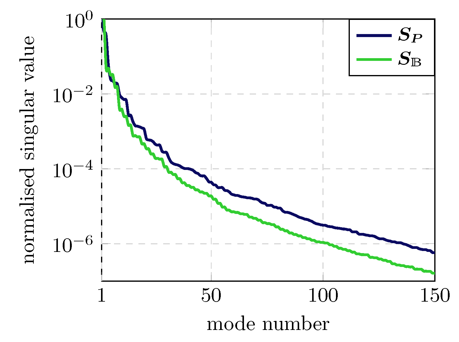
3.1. Reduced Basis
3.2. Galerkin ROM
4. Hyper-Reduction
4.1. Discrete Empirical Interpolation Method
4.2. Gappy POD
4.3. GNAT
4.4. Empirical Cubature
4.5. Reduced Integration Domain
5. Numerical Results
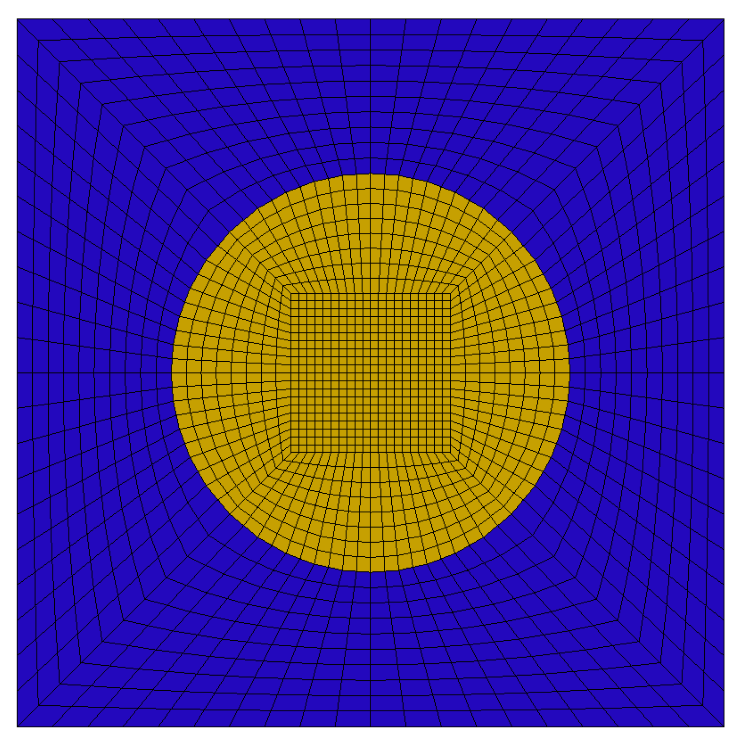
5.1. Test Problem
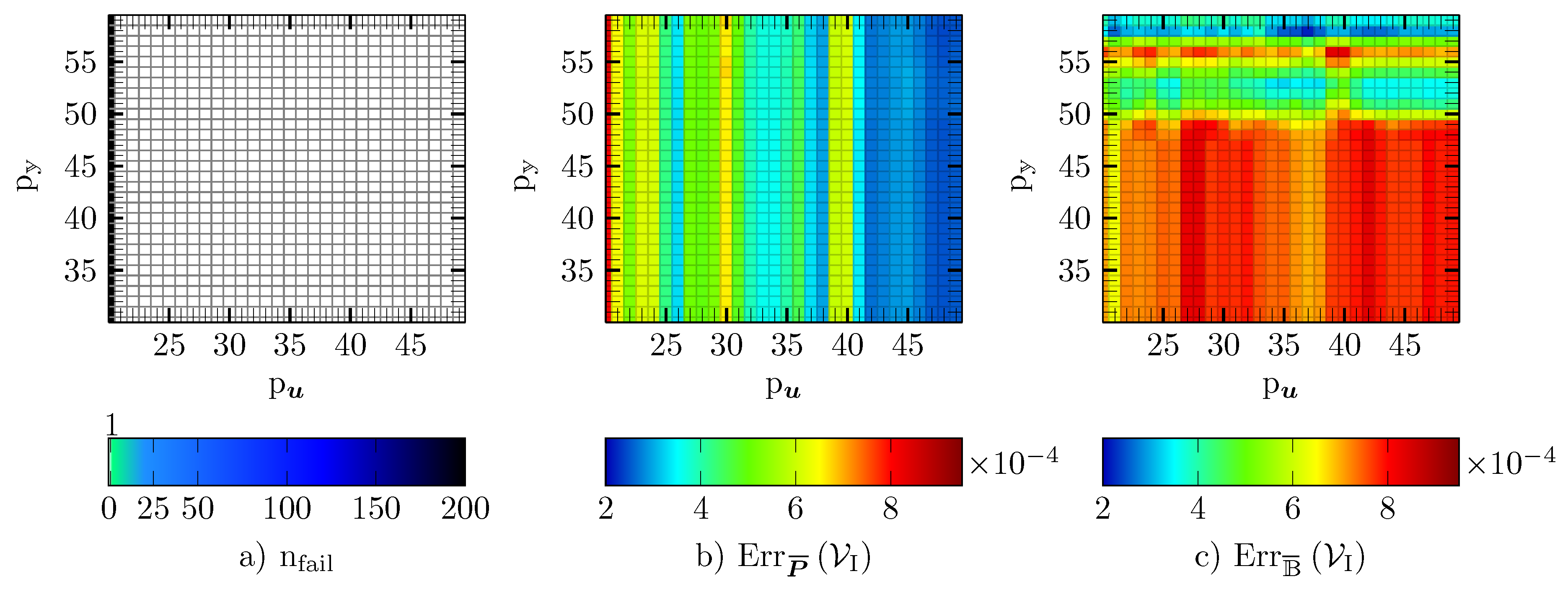
5.2. Validation of Galerkin ROM
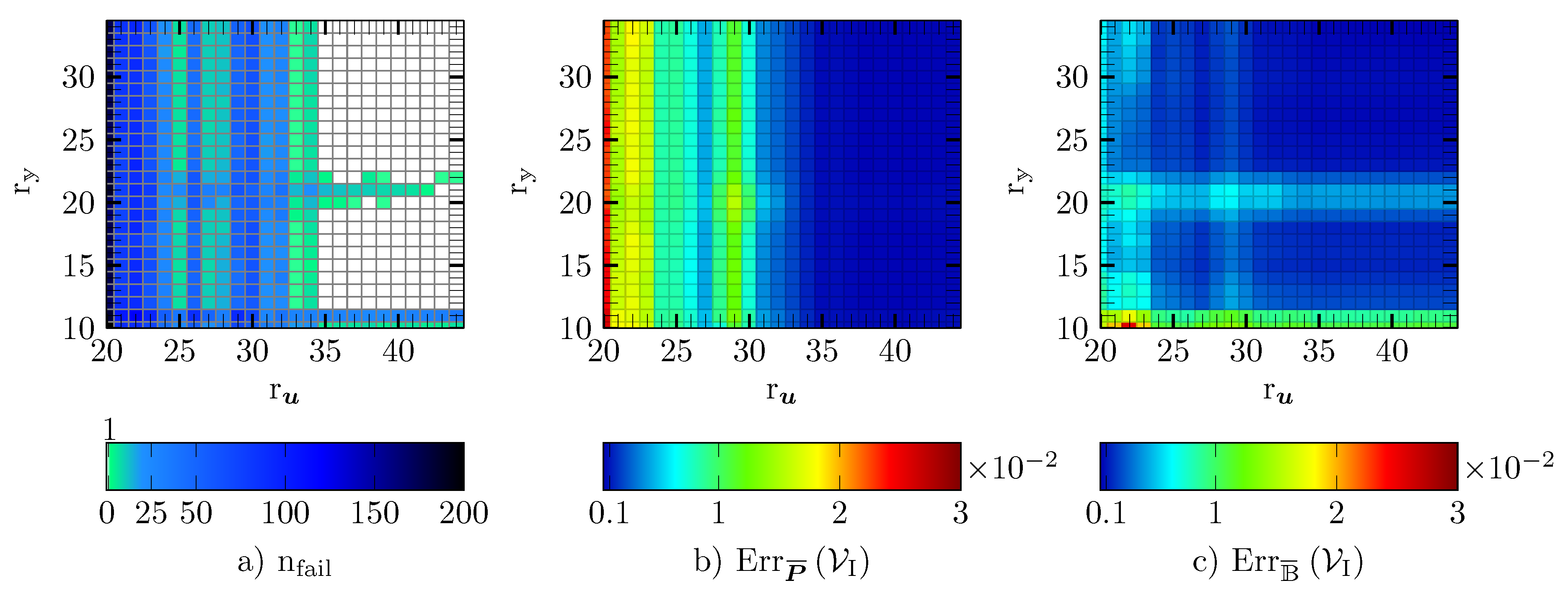
5.3. DEIM
5.4. Gappy POD
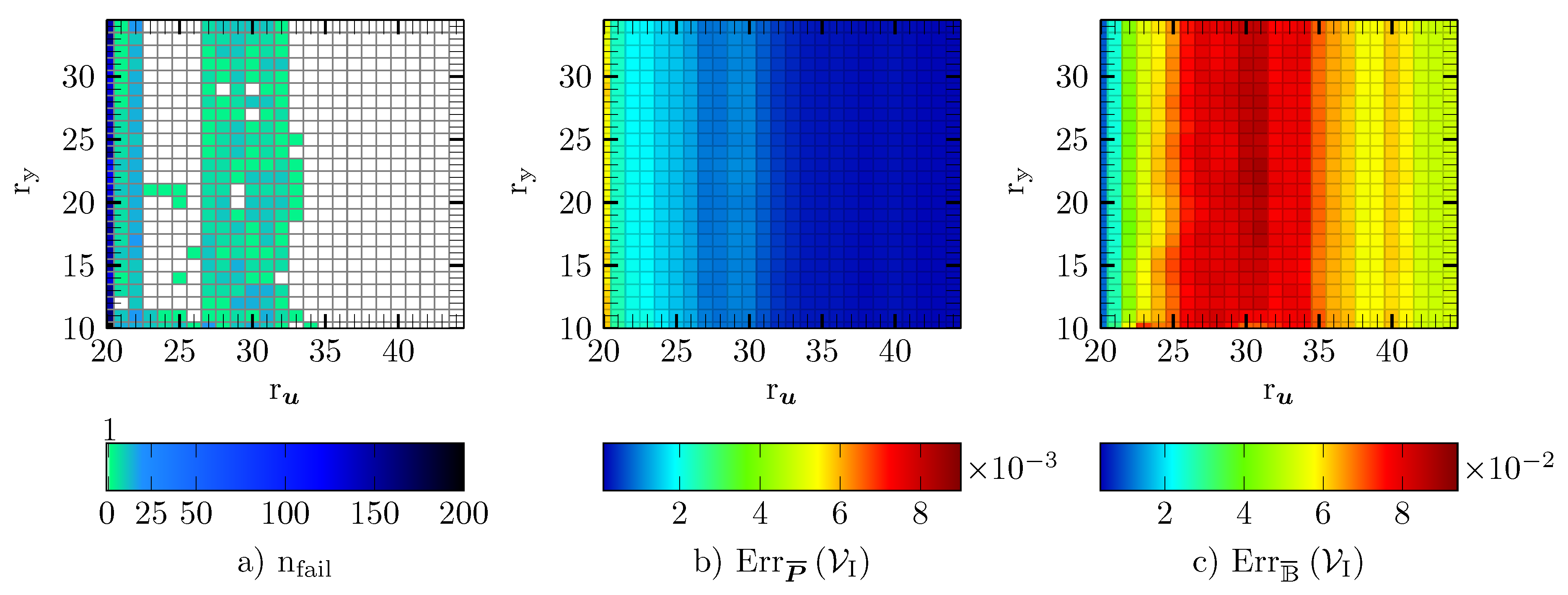
5.5. GNAT
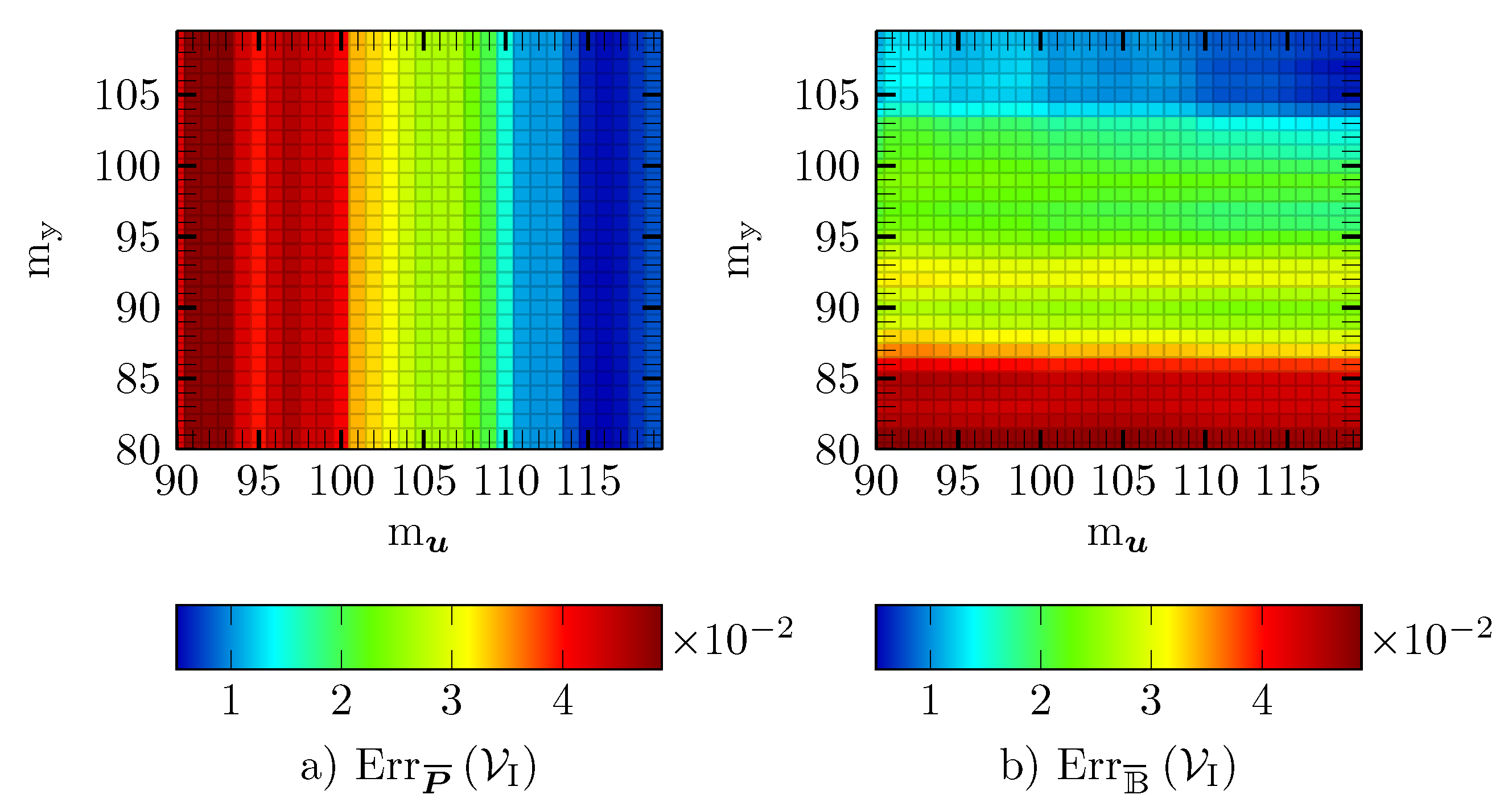
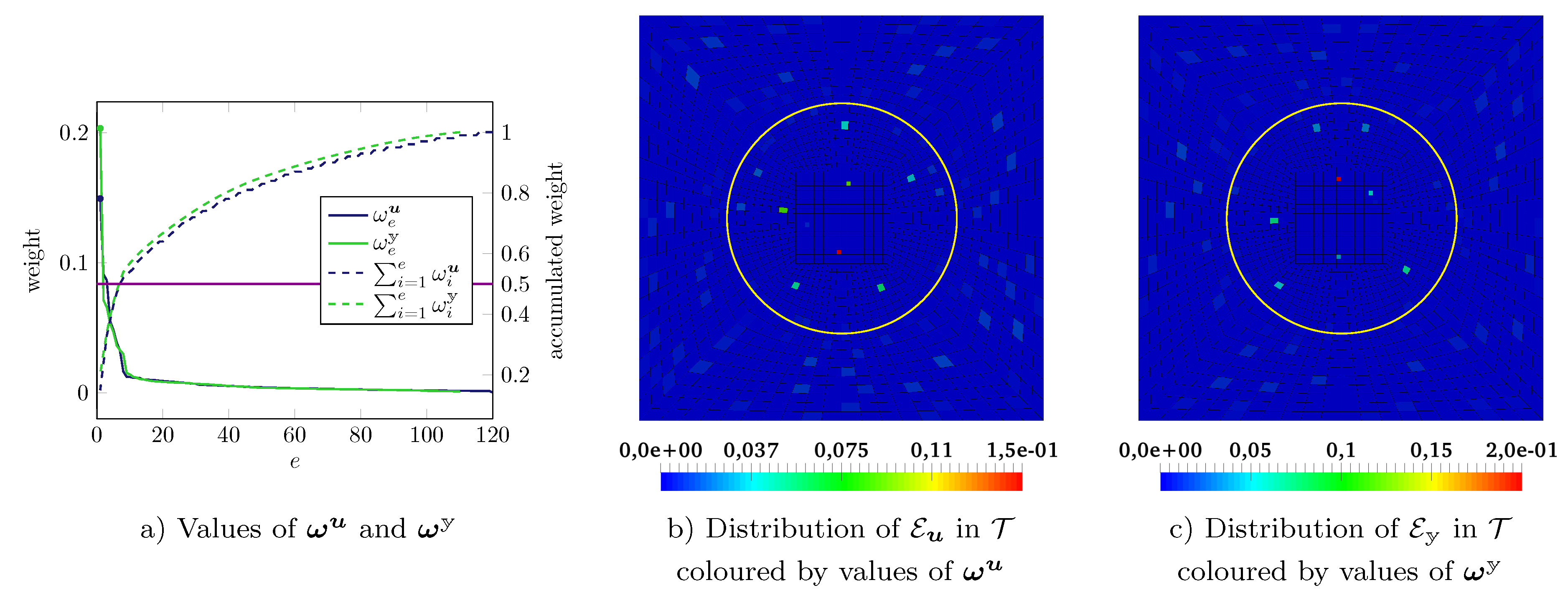
5.6. Empirical Cubature
5.7. Reduced Integration Domain
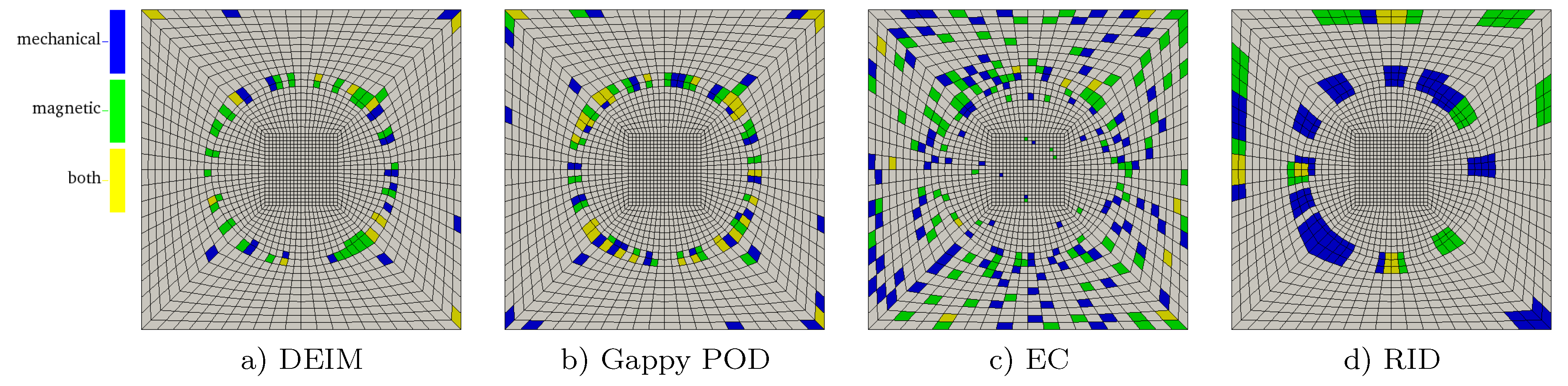
5.8. Comparison of the Hyper-Reduction Methods
6. Conclusions
Author Contributions
Funding
Conflicts of Interest
Abbreviations
| MRE | Magneto-Rheological Elastomer |
| BVP | Boundary Value Problem |
| RVE | Representative Volume Element |
| ROM | Reduced-Order Model |
| FEM | Finite Element Method |
| DoF | Degree of Freedom |
| FOM | Full-Order Model |
| pPDE | parametrised Partial Differential Equation |
| POD | Proper Orthogonal Decomposition |
| SVD | Singular Value Decomposition |
| EIM | Empirical Interpolation Method |
| DEIM | Discrete Empirical Interpolation Method |
| GNAT | Gauss–Newton with Approximated Tensors |
| EC | Empirical Cubature |
| ECSW | Energy-Conserving Sampling and Weighting |
| RID | Reduced Integration Domain |
Appendix A. DEIM
| Algorithm A1: DEIM Algorithm |
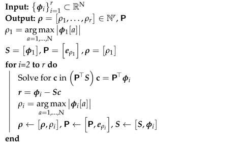 |
Appendix B. Gappy POD and GNAT
| Algorithm A2: Greedy Point Search |
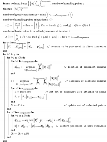 |
Appendix C. Empirical Cubature
| Algorithm A3: Greedy Mesh Sampling |
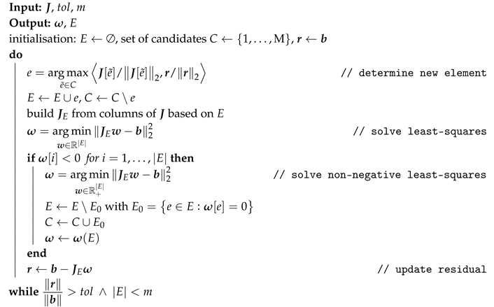 |
Appendix D. Reduced Integration Domain
| Algorithm A4: Determining Reduced Integration Domain |
| Input: POD basis , number of neighbouring element layers l Output: , get DEIM indices by applying Algorithm A1 to // collect elements containing the DEIM indices for i=1 to l do | // add neighbouring elements end setup based on interior DoFs (primary) in |
References
- Feyel, F.; Chaboche, J.L. FE2 multiscale approach for modelling the elastoviscoplastic behaviour of long fibre SiC/Ti composite materials. Comput. Methods Appl. Mech. Eng. 2000, 183, 309–330. [Google Scholar] [CrossRef]
- Saeb, S.; Steinmann, P.; Javili, A. Aspects of computational homogenization at finite deformations: A unifying review from Reuss’ to Voigt’s bound. Appl. Mech. Rev. 2016, 68, 050801. [Google Scholar] [CrossRef]
- Bartuschat, D.; Gmeiner, B.; Thoennes, D.; Kohl, N.; Rüde, U.; Drzisga, D.; Huber, M.; John, L.; Waluga, C.; Wohlmuth, B.I.; et al. A Finite Element Multigrid Framework for Extreme-Scale Earth Mantle Convection Simulations. In Proceedings of the SIAM Conference on Parallel Processing for Scientific Computing (SIAM PP 18), Tokyo, Japan, 7–10 March 2018. [Google Scholar]
- Michel, J.C.; Suquet, P. A model-reduction approach in micromechanics of materials preserving the variational structure of constitutive relations. J. Mech. Phys. Solids 2016, 90, 254–285. [Google Scholar] [CrossRef]
- Fritzen, F.; Leuschner, M. Reduced basis hybrid computational homogenization based on a mixed incremental formulation. Comput. Methods Appl. Mech. Eng. 2013, 260, 143–154. [Google Scholar] [CrossRef]
- Chinesta, F.; Ammar, A.; Leygue, A.; Keunings, R. An overview of the proper generalized decomposition with applications in computational rheology. J. Non-Newton. Fluid Mech. 2011, 166, 578–592. [Google Scholar] [CrossRef]
- Cremonesi, M.; Néron, D.; Guidault, P.A.; Ladevèze, P. A PGD-based homogenization technique for the resolution of nonlinear multiscale problems. Comput. Methods Appl. Mech. Eng. 2013, 267, 275–292. [Google Scholar] [CrossRef]
- Sirovich, L. Turbulence and the Dynamics of Coherent Structures Part I: Coherent Structures. Q. Appl. Math. 1987, 45, 561–571. [Google Scholar] [CrossRef]
- Himpe, C.; Leibner, T.; Rave, S. Hierarchical Approximate Proper Orthogonal Decomposition. SIAM J. Sci. Comput. 2018, 40, A3267–A3292. [Google Scholar] [CrossRef]
- Paul-Dubois-Taine, A.; Amsallem, D. An adaptive and efficient greedy procedure for the optimal training of parametric reduced-order models. Int. J. Numer. Methods Eng. 2014, 102, 1262–1292. [Google Scholar] [CrossRef]
- Brands, B.; Mergheim, J.; Steinmann, P. Reduced-order modelling for linear heat conduction with parametrised moving heat sources. GAMM-Mitteilungen 2016, 39, 170–188. [Google Scholar] [CrossRef]
- Hesthaven, J.S.; Rozza, G.; Stamm, B. Certified Reduced Basis Methods for Parametrized Partial Differential Equations; Springer: Cham, Switzerland, 2017. [Google Scholar]
- Quarteroni, A.; Manzoni, A.; Negri, F. Reduced Basis Methods for Partial Differential Equations: An Introduction; Springer: Cham, Switzerland, 2015; Volume 92. [Google Scholar]
- Rozza, G.; Huynh, D.B.P.; Patera, A.T. Reduced basis approximation and a posteriori error estimation for affinely parametrized elliptic coercive partial differential equations. Arch. Comput. Methods Eng. 2008, 15, 229–275. [Google Scholar] [CrossRef]
- Grepl, M.A.; Patera, A.T. A posteriori error bounds for reduced-basis approximations of parametrized parabolic partial differential equations. ESAIM Math. Model. Numer. Anal. 2005, 39, 157–181. [Google Scholar] [CrossRef]
- Yvonnet, J.; He, Q.C. The reduced model multiscale method (R3M) for the nonlinear homogenization of hyperelastic media at finite strains. J. Comput. Phys. 2007, 223, 341–368. [Google Scholar] [CrossRef]
- Radermacher, A.; Bednarcyk, B.A.; Stier, B.; Simon, J.; Zhou, L.; Reese, S. Displacement-based multiscale modeling of fiber-reinforced composites by means of proper orthogonal decomposition. Adv. Model. Simul. Eng. Sci. 2016, 3, 29. [Google Scholar] [CrossRef]
- Grepl, M.A.; Maday, Y.; Nguyen, N.C.; Patera, A.T. Efficient reduced-basis treatment of nonaffine and nonlinear partial differential equations. ESAIM M2AN 2007, 41, 575–605. [Google Scholar] [CrossRef]
- Chaturantabut, S.; Sorensen, D.C. Nonlinear Model Reduction via Discrete Empirical Interpolation. SIAM J. Sci. Comput. 2010, 32, 2737–2764. [Google Scholar] [CrossRef]
- Everson, R.; Sirovich, L. Karhunen-Loeve procedure for gappy data. J. Opt. Soc. Am. A 1995, 12, 1657–1664. [Google Scholar] [CrossRef]
- Carlberg, K.; Farhat, C.; Cortial, J.; Amsallem, D. The GNAT method for nonlinear model reduction: Effective implementation and application to computational fluid dynamics and turbulent flows. J. Comput. Phys. 2013, 242, 623–647. [Google Scholar] [CrossRef]
- Goury, O.; Amsallem, D.; Bordas, S.P.A.; Liu, W.K.; Kerfriden, P. Automatised selection of load paths to construct reduced-order models in computational damage micromechanics: From dissipation-driven random selection to Bayesian optimization. Comput. Mech. 2016, 58, 213–234. [Google Scholar] [CrossRef]
- Ghavamian, F.; Tiso, P.; Simone, A. POD–DEIM model order reduction for strain-softening viscoplasticity. Comput. Methods Appl. Mech. Eng. 2017, 317, 458–479. [Google Scholar] [CrossRef]
- Tiso, P.; Rixen, D.J. Discrete Empirical Interpolation Method for Finite Element Structural Dynamics. In Topics in Nonlinear Dynamics, Volume 1: Proceedings of the 31st IMAC, A Conference on Structural Dynamics, Garden Grove, CA, USA, 11–14 February 2013; Kerschen, G., Adams, D., Carrella, A., Eds.; Springer: New York, NY, USA, 2013; pp. 203–212. [Google Scholar]
- Hernández, J.; Oliver, J.; Huespe, A.; Caicedo, M.; Cante, J. High-performance model reduction techniques in computational multiscale homogenization. Comput. Methods Appl. Mech. Eng. 2014, 276, 149–189. [Google Scholar] [CrossRef]
- Soldner, D.; Brands, B.; Zabihyan, R.; Steinmann, P.; Mergheim, J. A numerical study of different projection-based model reduction techniques applied to computational homogenisation. Comput. Mech. 2017, 60, 613–625. [Google Scholar] [CrossRef]
- An, S.S.; Kim, T.; James, D.L. Optimizing Cubature for Efficient Integration of Subspace Deformations. ACM Trans. Graph. 2008, 27, 165. [Google Scholar] [CrossRef] [PubMed]
- Farhat, C.; Avery, P.; Chapman, T.; Cortial, J. Dimensional reduction of nonlinear finite element dynamic models with finite rotations and energy-based mesh sampling and weighting for computational efficiency. Int. J. Numer. Methods Eng. 2014, 98, 625–662. [Google Scholar] [CrossRef]
- Hernández, J.; Caicedo, M.; Ferrer, A. Dimensional hyper-reduction of nonlinear finite element models via empirical cubature. Comput. Methods Appl. Mech. Eng. 2017, 313, 687–722. [Google Scholar] [CrossRef]
- Van Tuijl, R.A.; Remmers, J.J.C.; Geers, M.G.D. Integration efficiency for model reduction in micro-mechanical analyses. Comput. Mech. 2017, 62, 151–169. [Google Scholar] [CrossRef]
- Ryckelynck, D. A priori hyperreduction method: An adaptive approach. J. Comput. Phys. 2005, 202, 346–366. [Google Scholar] [CrossRef]
- Ryckelynck, D. Hyper-reduction of mechanical models involving internal variables. Int. J. Numer. Methods Eng. 2009, 77, 75–89. [Google Scholar] [CrossRef]
- Ryckelynck, D.; Benziane, D.M. Multi-level A Priori Hyper-Reduction of mechanical models involving internal variables. Comput. Methods Appl. Mech. Eng. 2010, 199, 1134–1142. [Google Scholar] [CrossRef]
- Ryckelynck, D.; Lampoh, K.; Quilicy, S. Hyper-reduced predictions for lifetime assessment of elasto-plastic structures. Meccanica 2016, 51, 309–317. [Google Scholar] [CrossRef]
- Fritzen, F.; Haasdonk, B.; Ryckelynck, D.; Schöps, S. An Algorithmic Comparison of the Hyper-Reduction and the Discrete Empirical Interpolation Method for a Nonlinear Thermal Problem. Math. Comput. Appl. 2018, 23, 8. [Google Scholar] [CrossRef]
- Astrid, P.; Weiland, S.; Willcox, K.; Backx, T. Missing point estimation in models described by proper orthogonal decomposition. IEEE Trans. Autom. Control 2008, 53, 2237–2251. [Google Scholar] [CrossRef]
- Dimitriu, G.; Ştefănescu, R.; Navon, I.M. Comparative numerical analysis using reduced-order modeling strategies for nonlinear large-scale systems. J. Comput. Appl. Math. 2017, 310, 32–43. [Google Scholar] [CrossRef]
- Walter, B.L.; Pelteret, J.P.; Kaschta, J.; Schubert, D.W.; Steinmann, P. Preparation of magnetorheological elastomers and their slip-free characterization by means of parallel-plate rotational rheometry. Smart Mater. Struct. 2017, 26, 085004. [Google Scholar] [CrossRef]
- Chatzigeorgiou, G.; Javili, A.; Steinmann, P. Unified magnetomechanical homogenization framework with application to magnetorheological elastomers. Math. Mech. Solids 2014, 19, 193–211. [Google Scholar] [CrossRef]
- Zabihyan, R.; Mergheim, J.; Javili, A.; Steinmann, P. Aspects of computational homogenization in magneto-mechanics: Boundary conditions, RVE size and microstructure composition. Int. J. Solids Struct. 2018, 130, 105–121. [Google Scholar] [CrossRef]
- Javili, A.; Chatzigeorgiou, G.; Steinmann, P. Computational homogenization in magneto-mechanics. Int. J. Solids Struct. 2013, 50, 4197–4216. [Google Scholar] [CrossRef]
- Holmes, P.; Lumley, J.L.; Berkooz, G.; Rowley, C.W. Turbulence, Coherent Structures, Dynamical Systems and Symmetry; Cambridge University Press: Cambridge, UK, 2012. [Google Scholar]
- Volkwein, S. Proper Orthogonal Decomposition: Theory and Reduced-Order Modelling; Lecture Notes; University of Konstanz: Konstanz, Germany, 2013; Volume 4. [Google Scholar]
- Chaturantabut, S.; Sorensen, D. A State Space Error Estimate for POD-DEIM Nonlinear Model Reduction. SIAM J. Numer. Anal. 2012, 50, 46–63. [Google Scholar] [CrossRef]
- Wirtz, D.; Sorensen, D.; Haasdonk, B. A Posteriori Error Estimation for DEIM Reduced Nonlinear Dynamical Systems. SIAM J. Sci. Comput. 2014, 36, A311–A338. [Google Scholar] [CrossRef]
- Chapman, T.; Avery, P.; Collins, P.; Farhat, C. Accelerated mesh sampling for the hyper reduction of nonlinear computational models. Int. J. Numer. Methods Eng. 2017, 109, 1623–1654. [Google Scholar] [CrossRef]
- Alzetta, G.; Arndt, D.; Bangerth, W.; Boddu, V.; Brands, B.; Davydov, D.; Gassmöller, R.; Heister, T.; Heltai, L.; Kormann, K.; et al. The deal.II Library, Version 9.0. J. Numer. Math. 2018, 26, 173–183. [Google Scholar] [CrossRef]
- Stoyanov, M. Adaptive Sparse Grid Construction in a Context of Local Anisotropy and Multiple Hierarchical Parents. In Sparse Grids and Applications—Miami 2016; Garcke, J., Pflüger, D., Webster, C.G., Zhang, G., Eds.; Springer International Publishing: Cham, Switzerland, 2018; pp. 175–199. [Google Scholar]
- Garcke, J.; Griebel, M. Sparse Grids and Applications, 1st ed.; Lecture Notes in Computational Science and Engineering; Springer Science & Business Media: Cham, Switzerland, 2012; Volume 88. [Google Scholar]
- Miehe, C. Numerical computation of algorithmic (consistent) tangent moduli in large-strain computational inelasticity. Comput. Methods Appl. Mech. Eng. 1996, 134, 223–240. [Google Scholar] [CrossRef]
- Pelteret, J.P.; Steinmann, P. Magneto-Active Polymers: Fabrication, Characterisation, Modelling and Simulation at the Micro- and Macro-Scale; In Preparation; de Gruyter Mouton: Berlin, Germany, 2019. [Google Scholar]


| Matrix | Inclusion | |
|---|---|---|
| 12 | 120 | |
| 8 | 80 | |
| 0.001 | 0.01 |
| 4541 | 12,841 | 33,193 | |
|---|---|---|---|
| l | 1 | 2 | 3 |
|---|---|---|---|
| DEIM | Gappy POD | EC | RID | |
|---|---|---|---|---|
| & | 50 & | 69 & | 120 & | 129 & |
| & | 1000 & 500 | 1468 & 734 | 3400 & 1700 | 1938 & 969 |
| 18 | 0 | 0 | 0 | |
| speed-up | 208 | 131 | 23 | 32 |
| DEIM | and |
|---|---|
| Gappy POD | and , and |
| EC | and |
| RID |
© 2019 by the authors. Licensee MDPI, Basel, Switzerland. This article is an open access article distributed under the terms and conditions of the Creative Commons Attribution (CC BY) license (http://creativecommons.org/licenses/by/4.0/).
Share and Cite
Brands, B.; Davydov, D.; Mergheim, J.; Steinmann, P. Reduced-Order Modelling and Homogenisation in Magneto-Mechanics: A Numerical Comparison of Established Hyper-Reduction Methods. Math. Comput. Appl. 2019, 24, 20. https://doi.org/10.3390/mca24010020
Brands B, Davydov D, Mergheim J, Steinmann P. Reduced-Order Modelling and Homogenisation in Magneto-Mechanics: A Numerical Comparison of Established Hyper-Reduction Methods. Mathematical and Computational Applications. 2019; 24(1):20. https://doi.org/10.3390/mca24010020
Chicago/Turabian StyleBrands, Benjamin, Denis Davydov, Julia Mergheim, and Paul Steinmann. 2019. "Reduced-Order Modelling and Homogenisation in Magneto-Mechanics: A Numerical Comparison of Established Hyper-Reduction Methods" Mathematical and Computational Applications 24, no. 1: 20. https://doi.org/10.3390/mca24010020
APA StyleBrands, B., Davydov, D., Mergheim, J., & Steinmann, P. (2019). Reduced-Order Modelling and Homogenisation in Magneto-Mechanics: A Numerical Comparison of Established Hyper-Reduction Methods. Mathematical and Computational Applications, 24(1), 20. https://doi.org/10.3390/mca24010020