Chaos and Relativistic Energy-Momentum of the Nonlinear Time Fractional Duffing Equation

Abstract

This paper studies the nonlinear fractional undamped Duffing equation. The Duffing equation is one of the fundamental equations in engineering. The geographical areas of this model represent chaos, relativistic energy-momentum, electrodynamics, and electromagnetic interactions. These properties have many benefits in different science fields. The equation depicts the energy of a point mass, which is well thought out as a periodically-forced oscillator. We employed twelve different techniques to the nonlinear fractional Duffing equation to find explicit solutions and approximate solutions. The stability of the solutions was also examined to show the ability of our obtained solutions in the application. The main goals here were to apply a novel computational method (modified auxiliary equation method) and compare the novel method with other methods via the solutions that were obtained by each of these methods.

1. Introduction

In this paper, we study the nonlinear fractional Duffing equation [1,2,3,4,5]. This equation describes the chaotic behavior of the motion of the hampered oscillator with a complexity potentially greater than for simple harmonious motion. We handle this with the force that results from the interaction between electrical charges. This force is called electromagnetism or Lorentz force, which includes magnetism and electricity as various phenomena of the equivalent source. The Duffing equation is named after Georg Duffing (1861–1944). He ascertained the relationship between the motion of a damped oscillator: Displacement, velocity, and acceleration. He derived his mathematical statement in the following form:

$$\begin{array}{c}{u}^{″}+au+b{u}^3+e{u}^{\prime }-fcos(\xi t)=0,\hfill \end{array}$$

(1)

where $[u,a,b,e,f,\xi ,u^3]$ represent a displacement in time, linear stiffness, the amount of nonlinearity in the regenerating force, a quantity of damping, the amplitude of the repeated driving force, the angular frequency of the occasional driving force, and the Duffing term, respectively. Under specific conditions on the previous parameters, we can turn it into the undamped and unforced Duffing equation. Many approaches have been used to solve this equation, namely the Fourier series or techniques, such as the Frobenius, Euler, Runge–Kutta, homotopy analysis, Poincaré–Lindstedt, or Lindstedt–Poincaré methods. This model can be reduced to other models, like the Landau–Ginzburg–Higgs, Klein–Gordon, and sine-Gordon equations.

According to the various application fields of nonlinear partial differential equations, many methods have been discovered and derived to study the exact and approximate solutions; for more details about some of these methods, see References [6,7,8,9,10,11,12,13,14,15,16,17,18,19,20,21,22,23,24]. In this research, we applied twelve methods to our nonlinear fractional unforced Duffing equation to study the properties of solutions and also the convergence among our solutions. We studied the stability of solutions to show the ability with respect to the model’s applications.

The strategy in this paper is summarized as follows: In Section 2, we describe how we applied twelve different techniques to the nonlinear fractional unforced Duffing equation. In Section 3, we examine the stability of the solutions of our model and draw some of the figures to indicate their properties. In Section 4, we discuss our obtained solutions to present the convergence among them. In Section 5, we provide the conclusion of our paper.

2. Application

In this part of our research, we applued eleven different methods to the nonlinear time fractional Duffing equation, which has the following formula:

$$\begin{array}{c}{D}_{tt}^{2\alpha }u+au+b{u}^3=0.\hfill \end{array}$$

(2)

Converting the fractional nonlinear partial differential equation to the integer order nonlinear partial differential equation using the following conformable fractional derivative $[u(x,t)=u(\mathsf{\Theta }),\mathsf{\Theta }=x+\frac{c{t}^{\alpha }}{\alpha }]$ (for more details about this kind of derivatives see References [25,26,27,28,29]), we get:

$$\begin{array}{c}{c}^2{u}^{″}+au+b{u}^3=0.\hfill \end{array}$$

(3)

Calculating the homogeneous balance value of Equation (3), we get $N=1$.

2.1. Exp $(-\varphi (\mathsf{\Theta }))$-Expansion Method

Applying this method enables us to put the general solution of Equation (3) in the next formula:

$$\begin{array}{c}u(\mathsf{\Theta })=a_1{e}^{-\varphi (\mathsf{\Theta })}+a_0.\hfill \end{array}$$

(4)

Handling Equation (3) using Equation (4) and its derivatives, we convert Equation (3) to a polynomial function of $e^{(-\varphi (\mathsf{\Theta }))}$. Gathering all coefficients of terms that have a same degree and equating them to zero, and solving the obtained system of equation, we get:

$$a_0\to \frac{\sqrt{-a-2c^2\mu }}{\sqrt{b}},a_1\to \frac{\sqrt{2}c\sqrt{-a-2c^2\mu }}{\sqrt{b}\sqrt{a+2c^2\mu }},\lambda \to \frac{\sqrt{2}\sqrt{a+2c^2\mu }}{c},\mathrm{where}(a+2c^2\mu >0\mathrm{and}b<0).$$

According to the values of these parameters, the solitary solutions of Equation (2) are organized as follows:

When $[{\lambda }^2-4\mu >0\mathrm{and}\mu \ne 0]$:

$$\begin{array}{c}u(x,t)=\frac{\sqrt{-a-2c^2\mu }(1-\frac{2c\mu }{\sqrt{\frac{a}{2}+c^2\mu }(\sqrt{{\lambda }^2-4\mu }tanh(\frac{1}{2}\sqrt{{\lambda }^2-4\mu }(\frac{c{t}^{\alpha }}{\alpha }+{\vartheta }_0+x))+\lambda -2\mu )})}{\sqrt{b}},\hfill \end{array}$$

(5)

$$\begin{array}{c}u(x,t)=\frac{\sqrt{-a-2c^2\mu }(1-\frac{2c\mu }{\sqrt{\frac{a}{2}+c^2\mu }(\sqrt{{\lambda }^2-4\mu }coth(\frac{1}{2}\sqrt{{\lambda }^2-4\mu }(\frac{c{t}^{\alpha }}{\alpha }+{\vartheta }_0+x))+\lambda -2\mu )})}{\sqrt{b}}.\hfill \end{array}$$

(6)

When $[{\lambda }^2-4\mu =0,\mu \ne 0\mathrm{and}\lambda \ne 0]$:

$$\begin{array}{c}u(x,t)=\frac{\sqrt{-a-2c^2\mu }(\frac{c\lambda (\frac{1}{\frac{c\lambda t^{\alpha }}{\alpha }+\lambda (\frac{c{t}^{\alpha }}{\alpha }+{\vartheta }_0)+\lambda x+2}-\frac{1}{2})}{\sqrt{\frac{a}{2}+c^2\mu }}+1)}{\sqrt{b}}.\hfill \end{array}$$

(7)

When $[{\lambda }^2-4\mu <0\mathrm{and}\mu \ne 0]$:

$$\begin{array}{c}u(x,t)=\frac{\sqrt{-a-2c^2\mu }(1-\frac{2c\mu }{\sqrt{\frac{a}{2}+c^2\mu }(\lambda -\sqrt{4\mu -{\lambda }^2}tan(\frac{1}{2}\sqrt{4\mu -{\lambda }^2}(\frac{c{t}^{\alpha }}{\alpha }+{\vartheta }_0+x)))})}{\sqrt{b}},\hfill \end{array}$$

(8)

$$\begin{array}{c}u(x,t)=\frac{\sqrt{-a-2c^2\mu }(1-\frac{2c\mu }{\sqrt{\frac{a}{2}+c^2\mu }(\lambda -\sqrt{4\mu -{\lambda }^2}cot(\frac{1}{2}\sqrt{4\mu -{\lambda }^2}(\frac{c{t}^{\alpha }}{\alpha }+{\vartheta }_0+x)))})}{\sqrt{b}}.\hfill \end{array}$$

(9)

2.2. Improved F-Expansion Method

Applying this method enables us to put the general solution of Equation (3) in the next formula:

$$\begin{array}{c}u(\mathsf{\Theta })=\frac{a_{-1}}{\mu +\varphi (\mathsf{\Theta })}+a_1(\mu +\varphi (\mathsf{\Theta }))+a_0.\hfill \end{array}$$

(10)

Handling Equation (3) using Equation (10) and its derivatives, we convert Equation (3) to a polynomial function of $\varphi (\mathsf{\Theta })$. Gathering all coefficients of terms that have a same degree and equating them to zero, and solving the obtained system of equation, we get:

Family I:

$$a_{-1}\to \frac{\sqrt{a}({\mu }^2+r)}{\sqrt{b}\sqrt{r}},a_0\to -\frac{\sqrt{a}\mu }{\sqrt{b}\sqrt{r}},a_1\to 0,c\to -\frac{i\sqrt{a}}{\sqrt{2}\sqrt{r}},\mathrm{where}(a<0,b<0\mathrm{and}r>0).$$

According to the values of these parameters, the solitary solutions of Equation (2) are organized as follows:

$$\begin{array}{c}u(x,t)=\frac{\sqrt{a}(-\mu +\frac{{\mu }^2+r}{\mu +\sqrt{r}tan(\sqrt{r}x-\frac{i\sqrt{a}{t}^{\alpha }}{\sqrt{2}\alpha })})}{\sqrt{b}\sqrt{r}},\hfill \end{array}$$

(11)

$$\begin{array}{c}u(x,t)=\frac{\sqrt{a}(-\mu +\frac{{\mu }^2+r}{\mu -\sqrt{r}cot(\sqrt{r}x-\frac{i\sqrt{a}{t}^{\alpha }}{\sqrt{2}\alpha })})}{\sqrt{b}\sqrt{r}}.\hfill \end{array}$$

(12)

Family II:

$$a_{-1}\to 0,a_0\to \frac{\sqrt{a}\mu }{\sqrt{b}\sqrt{r}},a_1\to -\frac{\sqrt{a}}{\sqrt{b}\sqrt{r}},c\to -\frac{i\sqrt{a}}{\sqrt{2}\sqrt{r}},\mathrm{where}(a<0\mathrm{and}b<0).$$

According to the values of these parameters, the solitary solutions of Equation (2) are organized as follows:

$$\begin{array}{c}u(x,t)=-\frac{\sqrt{a}tan(\sqrt{r}x-\frac{i\sqrt{a}{t}^{\alpha }}{\sqrt{2}\alpha })}{\sqrt{b}},\hfill \end{array}$$

(13)

$$\begin{array}{c}u(x,t)=\frac{\sqrt{a}cot(\sqrt{r}x-\frac{i\sqrt{a}{t}^{\alpha }}{\sqrt{2}\alpha })}{\sqrt{b}}.\hfill \end{array}$$

(14)

2.3. Extended $(\frac{G^{\prime }}{G})$-Expansion Method

Applying this method enables us to put the general solution of Equation (3) in the next formula:

$$\begin{array}{c}u(\mathsf{\Theta })=\frac{a_1{G}^{\prime }(\mathsf{\Theta })}{G(\mathsf{\Theta })}+a_0+b_1\sqrt{\sigma (\frac{G^{\prime }{(\mathsf{\Theta })}^2}{\mu G{(\mathsf{\Theta })}^2}+1)}.\hfill \end{array}$$

(15)

Handling Equation (3) using Equation (15) and its derivatives, we convert Equation (3) to apolynomial function of ${(\frac{G^{\prime }(\mathsf{\Theta })}{G(\mathsf{\Theta })})}^i{\left[\sqrt{\frac{\sigma G^{\prime }{(\mathsf{\Theta })}^2}{\mu G{(\mathsf{\Theta })}^2}+\sigma }\right]}^j$. Gathering all coefficients of terms that have a same degree and equating them to zero, and solving the obtained system of equation, we get:

Family I:

$$a_0\to 0,a_1\to -\frac{ic}{\sqrt{2}\sqrt{b}},b_1\to -\frac{\sqrt{a}}{\sqrt{b}\sqrt{\sigma }},\mu \to -\frac{2a}{c^2},\mathrm{where}(b<0\mathrm{and}a<0).$$

According to the values of these parameters, the solitary solutions of Equation (2) are organized as follows:

When $[\mu >0]$:

$$\begin{array}{c}u(x,t)=\frac{1}{2\sqrt{b}}\left[-2\sqrt{\frac{a}{\sigma }}\sqrt{\frac{(c_1^2+c_2^2)\sigma }{(c_{1}sin(\frac{\sqrt{2}\sqrt{-a}{t}^{\alpha }+\alpha \mu x}{\alpha \sqrt{\mu }})+c_{2}cos(\frac{\sqrt{2}\sqrt{-a}{t}^{\alpha }+\alpha \mu x}{\alpha \sqrt{\mu }})){}^2}}+\frac{i\sqrt{2}c\sqrt{\mu }(c_2-c_{1}cot(\frac{\sqrt{2}\sqrt{-a}{t}^{\alpha }+\alpha \mu x}{\alpha \sqrt{\mu }}))}{c_{2}cot(\frac{\sqrt{2}\sqrt{-a}{t}^{\alpha }+\alpha \mu x}{\alpha \sqrt{\mu }})+c_1}\right].\hfill \end{array}$$

(16)

When $[\mu <0]$:

$$\begin{array}{cc}u(x,t)=\hfill & \frac{1}{2\sqrt{b}}[-2\sqrt{\frac{a}{\sigma }}\sqrt{\frac{(c_1^2-c_2^2)\sigma }{(c_{1}cos(\frac{\sqrt{2}\sqrt{-a}{t}^{\alpha }+\alpha \mu x}{\alpha \sqrt{\mu }})+c_{2}sinh(\sqrt{-\mu }(\frac{\sqrt{2}\sqrt{-a}{t}^{\alpha }}{\alpha \mu }+x))){}^2}}\\ & -\frac{i\sqrt{2}c(c_2\sqrt{-\mu }cos(\frac{\sqrt{2}\sqrt{-a}{t}^{\alpha }+\alpha \mu x}{\alpha \sqrt{\mu }})-c_1\sqrt{\mu }sin(\frac{\sqrt{2}\sqrt{-a}{t}^{\alpha }+\alpha \mu x}{\alpha \sqrt{\mu }}))}{c_{1}cos(\frac{\sqrt{2}\sqrt{-a}{t}^{\alpha }+\alpha \mu x}{\alpha \sqrt{\mu }})+c_{2}sinh(\sqrt{-\mu }(\frac{\sqrt{2}\sqrt{-a}{t}^{\alpha }}{\alpha \mu }+x))}].\end{array}$$

(17)

Family II:

$$a_0\to 0,a_1\to 0,b_1\to -\frac{i\sqrt{2}\sqrt{a}}{\sqrt{b}\sqrt{\sigma }},\mu \to \frac{a}{c^2},\mathrm{where}(b<0).$$

According to the values of these parameters, the solitary solutions of Equation (2) are organized as follows:

When $[\mu >0]$:

$$\begin{array}{c}u(x,t)=-\frac{i\sqrt{2}\sqrt{a}\sqrt{\frac{(c_1^2+c_2^2)\sigma }{(c_{1}sin(\sqrt{\mu }(\frac{\sqrt{\frac{a}{\mu }}{t}^{\alpha }}{\alpha }+x))+c_{2}cos(\sqrt{\mu }(\frac{\sqrt{\frac{a}{\mu }}{t}^{\alpha }}{\alpha }+x))){}^2}}}{\sqrt{b}\sqrt{\sigma }}.\hfill \end{array}$$

(18)

When $[\mu <0]$:

$$\begin{array}{c}u(x,t)=-\frac{i\sqrt{2}\sqrt{a}\sqrt{\frac{(c_1^2-c_2^2)\sigma }{(c_{1}cos(\sqrt{\mu }(\frac{\sqrt{\frac{a}{\mu }}{t}^{\alpha }}{\alpha }+x))+c_{2}sinh(\sqrt{-\mu }(\frac{\sqrt{\frac{a}{\mu }}{t}^{\alpha }}{\alpha }+x))){}^2}}}{\sqrt{b}\sqrt{\sigma }}.\hfill \end{array}$$

(19)

2.4. Extended Tanh-Function Method

Applying this method enables us to put the general solution of Equation (3) in the next formula:

$$\begin{array}{c}u(\mathsf{\Theta })=\frac{a_{-1}}{\varphi (\mathsf{\Theta })}+a_1\varphi (\mathsf{\Theta })+a_0.\hfill \end{array}$$

(20)

Handling Equation (3) using Equation (20) and its derivatives, we convert Equation (3) to a polynomial function of $\varphi (\mathsf{\Theta })$. Gathering all coefficients of terms that have a same degree and equating them to zero, and solving the obtained system of equation, we get:

Family I:

$$a_0\to 0,a_1\to -\frac{i\sqrt{a}}{\sqrt{2}\sqrt{b}\sqrt{d}},a_{-1}\to -\frac{i\sqrt{a}\sqrt{d}}{\sqrt{2}\sqrt{b}},c\to -\frac{\sqrt{a}}{2\sqrt{d}},\mathrm{where}(b<0,a>0\mathrm{and}d>0).$$

According to the values of these parameters, the solitary solutions of Equation (2) are organized as follows:

$$\begin{array}{c}u(x,t)=\mp \frac{i\sqrt{2}\sqrt{a}csc(2\sqrt{d}(x-\frac{\sqrt{a}{t}^{\alpha }}{2\alpha \sqrt{d}}))}{\sqrt{b}}.\hfill \end{array}$$

(21)

Family II:

$$a_0\to 0,a_1\to \frac{\sqrt{a}}{\sqrt{b}\sqrt{d}},a_{-1}\to 0,c\to \frac{i\sqrt{a}}{\sqrt{2}\sqrt{d}},\mathrm{where}(d<0,a<0\mathrm{and}b<0).$$

According to the values of these parameters, the solitary solutions of Equation (2) are organized as follows:

$$\begin{array}{c}u(x,t)=\frac{\sqrt{a}tan(\sqrt{d}(x+\frac{i\sqrt{a}{t}^{\alpha }}{\sqrt{2}\alpha \sqrt{d}}))}{\sqrt{b}},\hfill \end{array}$$

(22)

$$\begin{array}{c}u(x,t)=-\frac{\sqrt{a}cot(\sqrt{d}(x+\frac{i\sqrt{a}{t}^{\alpha }}{\sqrt{2}\alpha \sqrt{d}}))}{\sqrt{b}}.\hfill \end{array}$$

(23)

2.5. Simplest Equation Method

Applying this method enables to put the general solution of Equation (3) in the next formula:

$$\begin{array}{c}u(\mathsf{\Theta })=a_{1}f(\mathsf{\Theta })+a_0.\hfill \end{array}$$

(24)

Handling Equation (3) using Equation (24) and its derivatives, we convert Equation (3) to a polynomial function of $f(\mathsf{\Theta })$. Gathering all coefficients of terms that have a same degree and equating them to zero, and solving the obtained system of equation, we get:

Case I:

$$a_1\to -\frac{i\sqrt{2}c}{\sqrt{b}},a\to -b{a}_0^2,c_1\to -\frac{i\sqrt{2}{a}_0\sqrt{b}}{c},\mathrm{where}(b<0\mathrm{and}c\ne 0).$$

According to the values of these parameters, the solitary solutions of Equation (2) are organized as follows:

When $[c_2\to -1]$:

$$\begin{array}{c}u(x,t)=a_0-\frac{ic{c}_1(tanh(\frac{1}{2}{c}_1(\frac{c{t}^{\alpha }}{\alpha }+x+\vartheta ))+1)}{\sqrt{2}\sqrt{b}}.\hfill \end{array}$$

(25)

$$\begin{array}{c}u(x,t)=a_0+\frac{ic{c}_1(tanh(\frac{1}{2}{c}_1(\frac{c{t}^{\alpha }}{\alpha }+x+\vartheta ))-1)}{\sqrt{2}\sqrt{b}}.\hfill \end{array}$$

(26)

Case II:

$$a_1\to -2a_0,c\to i\sqrt{2}{a}_0\sqrt{b},a\to -b{a}_0^2\mathrm{where}(b<0\mathrm{and}{a}_0\ne 0).$$

According to the values of these parameters, the solitary solutions of Equation (2) are organized as follows:

When $[c_1\to 1,c_2\to -1]$:

$$\begin{array}{c}u(x,t)=-a_{0}tanh(\frac{1}{2}(x+\frac{\sqrt{2}i{a}_0\sqrt{b}{t}^{\alpha }}{\alpha })).\hfill \end{array}$$

(27)

2.6. Extended Simplest Equation Method

Applying this method enables us to put the general solution of Equation (3) in the next formula:

$$\begin{array}{c}u(\mathsf{\Theta })=\frac{a_{-1}}{f(\mathsf{\Theta })}+a_{1}f(\mathsf{\Theta })+a_0.\hfill \end{array}$$

(28)

Handling Equation (3)using Equation (28) and its derivatives, we convert Equation (3) to a polynomial function of $f(\mathsf{\Theta })$. Gathering all coefficients of terms that have a same degree and equating them to zero, and solving the obtained system of equation, we get:

Family I:

$$a_{-1}\to 0,a_0\to -\frac{i\sqrt{a}\lambda }{\sqrt{b{\lambda }^2-4\alpha b\mu }},a_1\to -\frac{2i\sqrt{a}\mu }{\sqrt{b({\lambda }^2-4\alpha \mu )}},c\to -\frac{\sqrt{2}\sqrt{a}}{\sqrt{{\lambda }^2-4\alpha \mu }},$$

$$\mathrm{where}(a<0,b<0\mathrm{and}{\lambda }^2-4\alpha \mu <0).$$

According to the values of these parameters, the solitary solutions of Equation (2) are organized as follows:

When $[\lambda =0]$, while $[{\alpha }_1\mu >0]$:

$$\begin{array}{c}u(x,t)=-\frac{i\sqrt{a}\sqrt{{\alpha }_1\mu }tan(\sqrt{{\alpha }_1\mu }(\frac{\sqrt{a}\mu t^{\alpha }}{\sqrt{2}{(-\alpha \mu )}^{3/2}}+x+\vartheta ))}{\sqrt{\alpha (-b)\mu }},\hfill \end{array}$$

(29)

$$\begin{array}{c}u(x,t)=-\frac{i\sqrt{a}\sqrt{{\alpha }_1\mu }cot(\sqrt{{\alpha }_1\mu }(\frac{\sqrt{a}\mu t^{\alpha }}{\sqrt{2}{(-\alpha \mu )}^{3/2}}+x+\vartheta ))}{\sqrt{\alpha (-b)\mu }},\hfill \end{array}$$

(30)

while $[{\alpha }_1\mu <0]$:

$$\begin{array}{c}u(x,t)=-\frac{i\sqrt{a}\sqrt{{\alpha }_1(-\mu )}tanh(\sqrt{{\alpha }_1(-\mu )}(\frac{\sqrt{a}\mu t^{\alpha }}{\sqrt{2}{(-\alpha \mu )}^{3/2}}+x)\mp \frac{log(\vartheta )}{2})}{\sqrt{\alpha (-b)\mu }},\hfill \end{array}$$

(31)

$$\begin{array}{c}u(x,t)=-\frac{i\sqrt{a}\sqrt{{\alpha }_1(-\mu )}coth(\sqrt{{\alpha }_1(-\mu )}(\frac{\sqrt{a}\mu t^{\alpha }}{\sqrt{2}{(-\alpha \mu )}^{3/2}}+x)\mp \frac{log(\vartheta )}{2})}{\sqrt{\alpha (-b)\mu }}.\hfill \end{array}$$

(32)

When $[{\alpha }_1=0]$, while $[\lambda >0]$:

$$\begin{array}{c}u(x,t)=\frac{i\sqrt{a}\lambda (\frac{2}{\mu e^{\lambda (-\frac{\sqrt{2}\sqrt{a}{t}^{\alpha }}{\alpha \sqrt{{\lambda }^2-4\alpha \mu }}+x+\vartheta )}-1}+1)}{\sqrt{b({\lambda }^2-4\alpha \mu )}},\hfill \end{array}$$

(33)

$$\begin{array}{c}u(x,t)=-\frac{i\sqrt{a}(\lambda e^{\frac{\sqrt{2}\sqrt{a}\lambda t^{\alpha }}{\alpha \sqrt{{\lambda }^2-4\alpha \mu }}}+\mu (\lambda -2\mu )e^{\lambda (x+\vartheta )})}{\sqrt{b({\lambda }^2-4\alpha \mu )}(e^{\frac{\sqrt{2}\sqrt{a}\lambda t^{\alpha }}{\alpha \sqrt{{\lambda }^2-4\alpha \mu }}}+\mu e^{\lambda (x+\vartheta )})}.\hfill \end{array}$$

(34)

When $[4{\alpha }_1\mu >{\lambda }^2]$, while $[\mu >0]$:

$$\begin{array}{c}u(x,t)=-\frac{i\sqrt{a}\sqrt{4{\alpha }_1\mu -{\lambda }^2}tan(\frac{1}{2}\sqrt{4{\alpha }_1\mu -{\lambda }^2}(-\frac{\sqrt{2}\sqrt{a}{t}^{\alpha }}{\alpha \sqrt{{\lambda }^2-4\alpha \mu }}+x+\vartheta ))}{\sqrt{b({\lambda }^2-4\alpha \mu )}},\hfill \end{array}$$

(35)

$$\begin{array}{c}u(x,t)=-\frac{i\sqrt{a}\sqrt{4{\alpha }_1\mu -{\lambda }^2}cot(\frac{1}{2}\sqrt{4{\alpha }_1\mu -{\lambda }^2}(-\frac{\sqrt{2}\sqrt{a}{t}^{\alpha }}{\alpha \sqrt{{\lambda }^2-4\alpha \mu }}+x+\vartheta ))}{\sqrt{b({\lambda }^2-4\alpha \mu )}}.\hfill \end{array}$$

(36)

When $[4{\alpha }_1\mu <{\lambda }^2]$, while $[\mu >0]$:

$$\begin{array}{c}u(x,t)=-\frac{i\sqrt{a}(\sqrt{4{\alpha }_1\mu -{\lambda }^2}tan(\frac{1}{2}\sqrt{4{\alpha }_1\mu -{\lambda }^2}(-\frac{\sqrt{2}\sqrt{a}{t}^{\alpha }}{\alpha \sqrt{{\lambda }^2-4\alpha \mu }}+x+\vartheta ))+2\lambda )}{\sqrt{b({\lambda }^2-4\alpha \mu )}},\hfill \end{array}$$

(37)

$$\begin{array}{c}u(x,t)=-\frac{i\sqrt{a}(\sqrt{4{\alpha }_1\mu -{\lambda }^2}cot(\frac{1}{2}\sqrt{4{\alpha }_1\mu -{\lambda }^2}(-\frac{\sqrt{2}\sqrt{a}{t}^{\alpha }}{\alpha \sqrt{{\lambda }^2-4\alpha \mu }}+x+\vartheta ))+2\lambda )}{\sqrt{b({\lambda }^2-4\alpha \mu )}}.\hfill \end{array}$$

(38)

Family II:

$$a_{-1}\to \frac{2i\sqrt{a}\alpha }{\sqrt{b({\lambda }^2-4\alpha \mu )}},a_0\to \frac{i\sqrt{a}\lambda }{\sqrt{b{\lambda }^2-4\alpha b\mu }},a_1\to 0,c\to -\frac{\sqrt{2}\sqrt{a}}{\sqrt{{\lambda }^2-4\alpha \mu }},$$

$$\mathrm{where}(a<0\&b<0\&{\lambda }^2-4\alpha \mu ).$$

According to the values of these parameters, the solitary solutions of Equation (2) are organized as follows:

When $[\lambda =0]$, while $[{\alpha }_1\mu >0]$:

$$\begin{array}{c}u(x,t)=\frac{i\sqrt{a}\alpha \mu cot(\sqrt{{\alpha }_1\mu }(\frac{\sqrt{a}\mu t^{\alpha }}{\sqrt{2}{(-\alpha \mu )}^{3/2}}+x+\vartheta ))}{\sqrt{{\alpha }_1\mu }\sqrt{\alpha (-b)\mu }},\hfill \end{array}$$

(39)

$$\begin{array}{c}u(x,t)=\frac{i\sqrt{a}\alpha \mu tan(\sqrt{{\alpha }_1\mu }(\frac{\sqrt{a}\mu t^{\alpha }}{\sqrt{2}{(-\alpha \mu )}^{3/2}}+x+\vartheta ))}{\sqrt{{\alpha }_1\mu }\sqrt{\alpha (-b)\mu }},\hfill \end{array}$$

(40)

while $[{\alpha }_1\mu <0]$:

$$\begin{array}{c}u(x,t)=\frac{i\sqrt{a}\alpha \mu coth(\sqrt{{\alpha }_1(-\mu )}(\frac{\sqrt{a}\mu t^{\alpha }}{\sqrt{2}{(-\alpha \mu )}^{3/2}}+x)\mp \frac{ln(\vartheta )}{2})}{\sqrt{{\alpha }_1(-\mu )}\sqrt{\alpha (-b)\mu }},\hfill \end{array}$$

(41)

$$\begin{array}{c}u(x,t)=\frac{i\sqrt{a}\alpha \mu tanh(\sqrt{{\alpha }_1(-\mu )}(\frac{\sqrt{a}\mu t^{\alpha }}{\sqrt{2}{(-\alpha \mu )}^{3/2}}+x)\mp \frac{ln(\vartheta )}{2})}{\sqrt{{\alpha }_1(-\mu )}\sqrt{\alpha (-b)\mu }}.\hfill \end{array}$$

(42)

When $[{\alpha }_1=0]$, while $[\lambda >0]$:

$$\begin{array}{c}u(x,t)=\frac{i\sqrt{a}(2\alpha exp(-\lambda (-\frac{\sqrt{2}\sqrt{a}{t}^{\alpha }}{\alpha \sqrt{{\lambda }^2-4\alpha \mu }}+x+\vartheta ))-2\alpha \mu +{\lambda }^2)}{\lambda \sqrt{b({\lambda }^2-4\alpha \mu )}},\hfill \end{array}$$

(43)

$$\begin{array}{c}u(x,t)=-\frac{i\sqrt{a}(\alpha (\frac{2exp(-\lambda (-\frac{\sqrt{2}\sqrt{a}{t}^{\alpha }}{\alpha \sqrt{{\lambda }^2-4\alpha \mu }}+x+\vartheta ))}{\mu }+2)-\lambda )}{\sqrt{b({\lambda }^2-4\alpha \mu )}}.\hfill \end{array}$$

(44)

When $[4{\alpha }_1\mu >{\lambda }^2]$, while $[\mu >0]$:

$$\begin{array}{c}u(x,t)=\frac{i\sqrt{a}(\lambda -\frac{4\alpha \mu }{\lambda -\sqrt{4{\alpha }_1\mu -{\lambda }^2}tan(\frac{1}{2}\sqrt{4{\alpha }_1\mu -{\lambda }^2}(-\frac{\sqrt{2}\sqrt{a}{t}^{\alpha }}{\alpha \sqrt{{\lambda }^2-4\alpha \mu }}+x+\vartheta ))})}{\sqrt{b({\lambda }^2-4\alpha \mu )}},\hfill \end{array}$$

(45)

$$\begin{array}{c}u(x,t)=\frac{i\sqrt{a}(\lambda -\frac{4\alpha \mu }{\lambda -\sqrt{4{\alpha }_1\mu -{\lambda }^2}cot(\frac{1}{2}\sqrt{4{\alpha }_1\mu -{\lambda }^2}(-\frac{\sqrt{2}\sqrt{a}{t}^{\alpha }}{\alpha \sqrt{{\lambda }^2-4\alpha \mu }}+x+\vartheta ))})}{\sqrt{b({\lambda }^2-4\alpha \mu )}}.\hfill \end{array}$$

(46)

When $[4{\alpha }_1\mu <{\lambda }^2]$, while $[\mu >0]$:

$$\begin{array}{c}u(x,t)=\frac{i\sqrt{a}(\frac{4\alpha \mu }{\sqrt{4{\alpha }_1\mu -{\lambda }^2}tan(\frac{1}{2}\sqrt{4{\alpha }_1\mu -{\lambda }^2}(-\frac{\sqrt{2}\sqrt{a}{t}^{\alpha }}{\alpha \sqrt{{\lambda }^2-4\alpha \mu }}+x+\vartheta ))+\lambda }+\lambda )}{\sqrt{b({\lambda }^2-4\alpha \mu )}},\hfill \end{array}$$

(47)

$$\begin{array}{c}u(x,t)=\frac{i\sqrt{a}(\frac{4\alpha \mu }{\sqrt{4{\alpha }_1\mu -{\lambda }^2}cot(\frac{1}{2}\sqrt{4{\alpha }_1\mu -{\lambda }^2}(-\frac{\sqrt{2}\sqrt{a}{t}^{\alpha }}{\alpha \sqrt{{\lambda }^2-4\alpha \mu }}+x+\vartheta ))+\lambda }+\lambda )}{\sqrt{b({\lambda }^2-4\alpha \mu )}}.\hfill \end{array}$$

(48)

2.7. Extended Fan-Expansion Method

Applying this method enables us to put the general solution of Equation (3) in the next formula:

$$\begin{array}{c}u(\mathsf{\Theta })=a_1\varphi (\mathsf{\Theta })+a_0.\hfill \end{array}$$

(49)

Handling Equation (3) using Equation (49) and its derivatives, we convert Equation (3) to a polynomial function of $\varphi (\mathsf{\Theta })$. Gathering all coefficients of terms that have a same degree and equating them to zero, and solving the obtained system of equation, we get:

$$a_0\to \frac{\sqrt{a}p}{\sqrt{4bqr-b{p}^2}},a_1\to \frac{2\sqrt{a}q}{\sqrt{-b(p^2-4qr)}},c\to -\frac{\sqrt{2}\sqrt{a}}{\sqrt{p^2-4qr}},\mathrm{where}(p^2-4qr>0,b<0\mathrm{and}a>0).$$

According to the values of these parameters, the solitary solutions of Equation (2) are organized as follows:

When $[pq\ne 0\mathrm{and}{B}^2-A^2>0]$:

$$\begin{array}{c}u(x,t)=\frac{\sqrt{a}b{\left(p^2-4qr\right)}^{3/2}tanh\left(\frac{1}{2}x\sqrt{p^2-4qr}-\frac{\sqrt{a}{t}^{\alpha }}{\sqrt{2}\alpha }\right)}{{\left(-b\left(p^2-4qr\right)\right)}^{3/2}},\hfill \end{array}$$

(50)

$$\begin{array}{c}u(x,t)=\frac{\sqrt{a}b{\left(p^2-4qr\right)}^{3/2}coth\left(\frac{1}{2}x\sqrt{p^2-4qr}-\frac{\sqrt{a}{t}^{\alpha }}{\sqrt{2}\alpha }\right)}{{\left(-b\left(p^2-4qr\right)\right)}^{3/2}},\hfill \end{array}$$

(51)

$$\begin{array}{c}u(x,t)=\frac{\sqrt{a}b{\left(p^2-4qr\right)}^{3/2}\left(tanh\left(x\sqrt{p^2-4qr}-\frac{\sqrt{2}\sqrt{a}{t}^{\alpha }}{\alpha }\right)\pm i\sec \mathrm{h}\left(x\sqrt{p^2-4qr}-\frac{\sqrt{2}\sqrt{a}{t}^{\alpha }}{\alpha }\right)\right)}{{\left(-b\left(p^2-4qr\right)\right)}^{3/2}},\hfill \end{array}$$

(52)

$$\begin{array}{c}u(x,t)=\frac{\sqrt{a}b{\left(p^2-4qr\right)}^{3/2}\left(coth\left(x\sqrt{p^2-4qr}-\frac{\sqrt{2}\sqrt{a}{t}^{\alpha }}{\alpha }\right)\pm \csc \mathrm{h}\left(x\sqrt{p^2-4qr}-\frac{\sqrt{2}\sqrt{a}{t}^{\alpha }}{\alpha }\right)\right)}{{\left(-b\left(p^2-4qr\right)\right)}^{3/2}},\hfill \end{array}$$

(53)

$$\begin{array}{c}u(x,t)=\frac{\sqrt{a}\sqrt{p^2-4qr}tanh\left(\frac{\sqrt{2}\sqrt{a}{t}^{\alpha }-\alpha x\sqrt{p^2-4qr}}{4\alpha }\right)\left({coth}^2\left(\frac{\sqrt{2}\sqrt{a}{t}^{\alpha }-\alpha x\sqrt{p^2-4qr}}{4\alpha }\right)+1\right)}{2\sqrt{-b\left(p^2-4qr\right)}},\hfill \end{array}$$

(54)

$$\begin{array}{c}u(x,t)=\frac{\sqrt{a}\left(\sqrt{\left(A^2+B^2\right)\left(p^2-4qr\right)}-A\sqrt{p^2-4qr}cosh\left(x\sqrt{p^2-4qr}-\frac{\sqrt{2}\sqrt{a}{t}^{\alpha }}{\alpha }\right)\right)}{\sqrt{-b\left(p^2-4qr\right)}\left(Asinh\left(x\sqrt{p^2-4qr}-\frac{\sqrt{2}\sqrt{a}{t}^{\alpha }}{\alpha }\right)+B\right)},\hfill \end{array}$$

(55)

$$\begin{array}{c}u(x,t)=-\frac{\sqrt{a}\left(A\sqrt{p^2-4qr}sinh\left(x\sqrt{p^2-4qr}-\frac{\sqrt{2}\sqrt{a}{t}^{\alpha }}{\alpha }\right)+\sqrt{\left(B^2-A^2\right)\left(p^2-4qr\right)}\right)}{\sqrt{-b\left(p^2-4qr\right)}\left(Acosh\left(x\sqrt{p^2-4qr}-\frac{\sqrt{2}\sqrt{a}{t}^{\alpha }}{\alpha }\right)+B\right)},\hfill \end{array}$$

(56)

$$\begin{array}{c}u(x,t)=\frac{\sqrt{a}\left(p-\frac{4qr}{\sqrt{p^2-4qr}tanh\left(\frac{\sqrt{2}\sqrt{a}{t}^{\alpha }-\alpha x\sqrt{p^2-4qr}}{2\alpha }\right)+p}\right)}{\sqrt{-b\left(p^2-4qr\right)}},\hfill \end{array}$$

(57)

$$\begin{array}{c}u(x,t)=\frac{\sqrt{a}\left(p-\frac{4qr}{\sqrt{p^2-4qr}coth\left(\frac{\sqrt{2}\sqrt{a}{t}^{\alpha }-\alpha x\sqrt{p^2-4qr}}{2\alpha }\right)+p}\right)}{\sqrt{-b\left(p^2-4qr\right)}},\hfill \end{array}$$

(58)

$$\begin{array}{c}u(x,t)=\frac{\sqrt{a}\left(p-\frac{4qrcosh\left(x\sqrt{p^2-4qr}-\frac{\sqrt{2}\sqrt{a}{t}^{\alpha }}{\alpha }\right)}{-\sqrt{p^2-4qr}sinh\left(x\sqrt{p^2-4qr}-\frac{\sqrt{2}\sqrt{a}{t}^{\alpha }}{\alpha }\right)+\left(pcosh\left(x\sqrt{p^2-4qr}-\frac{\sqrt{2}\sqrt{a}{t}^{\alpha }}{\alpha }\right)\pm i\sqrt{p^2-4qr}\right)}\right)}{\sqrt{-b\left(p^2-4qr\right)}},\hfill \end{array}$$

(59)

$$\begin{array}{c}u(x,t)=\frac{\sqrt{a}\left(p-\frac{4qr}{p-\csc \mathrm{h}\left(x\sqrt{p^2-4qr}-\frac{\sqrt{2}\sqrt{a}{t}^{\alpha }}{\alpha }\right)\left(\sqrt{p^2-4qr}cosh\left(x\sqrt{p^2-4qr}-\frac{\sqrt{2}\sqrt{a}{t}^{\alpha }}{\alpha }\right)\pm \sqrt{p^2-4qr}\right)}\right)}{\sqrt{-b\left(p^2-4qr\right)}},\hfill \end{array}$$

(60)

$$\begin{array}{c}u(x,t)=\frac{\sqrt{a}\left(\left(p^2-4qr\right)sinh\left(\frac{1}{2}x\sqrt{p^2-4qr}-\frac{\sqrt{a}{t}^{\alpha }}{\sqrt{2}\alpha }\right)-p\sqrt{p^2-4qr}cosh\left(2x\sqrt{p^2-4qr}-\frac{2\sqrt{2}\sqrt{a}{t}^{\alpha }}{\alpha }\right)\right)}{\sqrt{-b\left(p^2-4qr\right)}\left(psinh\left(\frac{1}{2}x\sqrt{p^2-4qr}-\frac{\sqrt{a}{t}^{\alpha }}{\sqrt{2}\alpha }\right)-\sqrt{p^2-4qr}cosh\left(2x\sqrt{p^2-4qr}-\frac{2\sqrt{2}\sqrt{a}{t}^{\alpha }}{\alpha }\right)\right)}.\end{array}$$

(61)

2.8. Generalized Kudryashov Method

Applying this method enables us to put the general solution of Equation (3) in the next formula:

$$\begin{array}{c}u(\mathsf{\Theta })=\frac{a_{2}Q{(\mathsf{\Theta })}^2+a_{1}Q(\mathsf{\Theta })+a_0}{b_{1}Q(\mathsf{\Theta })+b_0}.\hfill \end{array}$$

(62)

Handling Equation (3) using Equation (62) and its derivatives, we convert Equation (3) to a polynomial function of $Q(\mathsf{\Theta })$. Gathering all coefficients of terms that have a same degree and equating them to zero, and solving the obtained system of equation, we get:

Family I:

$$a_0\to \frac{i\sqrt{a}{b}_0}{\sqrt{b}},a_1\to 0,a_2\to -\frac{4i\sqrt{a}{b}_0}{\sqrt{b}},b_1\to 2b_0,c\to \sqrt{2}\sqrt{a},\mathrm{where}(b<0,a>0\mathrm{and}{b}_0\ne 0).$$

According to the values of these parameters, the solitary solutions of Equation (2) are organized as follows:

$$\begin{array}{c}u(x,t)=\frac{i\sqrt{a}(1-\frac{2}{A{e}^{\frac{\sqrt{2}\sqrt{a}{t}^{\alpha }}{\alpha }+x}+1})}{\sqrt{b}}.\hfill \end{array}$$

(63)

Family II:

$$a_0\to \frac{i(\frac{2\sqrt{a}{b}_0^2}{\sqrt{b}}-\frac{\sqrt{a}{b}_0{b}_1}{\sqrt{b}})}{2b_0-b_1},a_1\to -\frac{i\sqrt{a}(2b_0-b_1)}{\sqrt{b}},a_2\to \frac{2(ia{b}_1^2-2ia{b}_0{b}_1)}{2\sqrt{a}\sqrt{b}{b}_0-\sqrt{a}\sqrt{b}{b}_1},c\to -\sqrt{2}\sqrt{a},$$

$$\mathrm{where}(b<0,a>0,b_0\ne 0\mathrm{and}{b}_1\ne 0).$$

According to the values of these parameters, the solitary solutions of Equation (2) are organized as follows:

$$\begin{array}{c}u(x,t)=-\frac{i\sqrt{a}(1-\frac{2A{e}^x}{e^{\frac{\sqrt{2}\sqrt{a}{t}^{\alpha }}{\alpha }}+A{e}^x})}{\sqrt{b}}.\hfill \end{array}$$

(64)

Family III:

$$a_0\to 0,a_1\to \frac{2\sqrt{2}\sqrt{a}{b}_0}{\sqrt{b}},a_2\to -\frac{2\sqrt{2}\sqrt{a}{b}_0}{\sqrt{b}},b_1\to -2b_0,c\to -i\sqrt{a},\mathrm{where}(b<0,a<0\mathrm{and}{b}_0\ne 0).$$

According to the values of these parameters, the solitary solutions of Equation (2) are organized as follows:

$$\begin{array}{c}u(x,t)=\frac{2\sqrt{2}\sqrt{a}A{e}^{x+\frac{i\sqrt{a}{t}^{\alpha }}{\alpha }}}{\sqrt{b}(A^2{e}^{2x}-e^{\frac{2i\sqrt{a}{t}^{\alpha }}{\alpha }})}.\hfill \end{array}$$

(65)

Family IV:

$$a_0\to 0,a_1\to -\frac{i\sqrt{a}{b}_1}{\sqrt{b}},a_2\to \frac{2i\sqrt{a}{b}_1}{\sqrt{b}},b_0\to 0,c\to -\sqrt{2}\sqrt{a},\mathrm{where}(b<0,a<0\mathrm{and}{b}_1\ne 0).$$

According to the values of these parameters, the solitary solutions of Equation (2) are organized as follows:

$$\begin{array}{c}u(x,t)=\frac{i\sqrt{a}(1-\frac{2A{e}^x}{e^{\frac{\sqrt{2}\sqrt{a}{t}^{\alpha }}{\alpha }}+A{e}^x})}{\sqrt{b}}.\hfill \end{array}$$

(66)

Family V:

$$a_0\to -\frac{i\sqrt{a}{b}_0}{\sqrt{b}},a_1\to 0,a_2\to \frac{4i\sqrt{a}{b}_0}{\sqrt{b}},b_1\to 2b_0,c\to \sqrt{2}\sqrt{a},\mathrm{where}(b<0,a<0\mathrm{and}{b}_1\ne 0).$$

According to the values of these parameters, the solitary solutions of Equation (2) are organized as follows:

$$\begin{array}{c}u(x,t)=-\frac{i\sqrt{a}(1-\frac{2}{A{e}^{\frac{\sqrt{2}\sqrt{a}{t}^{\alpha }}{\alpha }+x}+1})}{\sqrt{b}}.\hfill \end{array}$$

(67)

2.9. Generalized Riccati Expansion Method

Applying this method enables us to put the general solution of Equation (3) in the next formula:

$$\begin{array}{c}u(\mathsf{\Theta })=a_{1}Q(\mathsf{\Theta })+a_0+\frac{b_1}{Q(\mathsf{\Theta })}.\hfill \end{array}$$

(68)

Handling Equation (3) using Equation (68) and its derivatives, we convert Equation (3) to a polynomial function of $Q(\mathsf{\Theta })$. Gathering all coefficients of terms that have a same degree and equating them to zero, and solving the obtained system of equation, we get:

$$a_0\to -\frac{\sqrt{a}p}{\sqrt{4bqr-b{p}^2}},a_1\to -\frac{2\sqrt{a}q}{\sqrt{-b(p^2-4qr)}},b_1\to 0,c\to -\frac{\sqrt{2}\sqrt{a}}{\sqrt{p^2-4qr}},\mathrm{where}(p^2-4qr>0,b<0\mathrm{and}a>0).$$

According to the values of these parameters, the solitary solutions of Equation (2) are organized as follows:

When $[p\ne 0,q\ne 0,r\ne 0\mathrm{and}{B}^2-A^2>0]$:

$$\begin{array}{c}u(x,t)=\frac{\sqrt{a}\sqrt{\Delta }tanh(\frac{1}{2}\sqrt{\Delta }(x-\frac{\sqrt{2}\sqrt{a}{t}^{\alpha }}{\alpha \sqrt{p^2-4qr}}))}{\sqrt{-b(p^2-4qr)}},\hfill \end{array}$$

(69)

$$\begin{array}{c}u(x,t)=\frac{\sqrt{a}\sqrt{\Delta }coth(\frac{1}{2}\sqrt{\Delta }(x-\frac{\sqrt{2}\sqrt{a}{t}^{\alpha }}{\alpha \sqrt{p^2-4qr}}))}{\sqrt{-b(p^2-4qr)}},\hfill \end{array}$$

(70)

$$\begin{array}{c}u(x,t)=\frac{\sqrt{a}\sqrt{\Delta }(tanh(\sqrt{\Delta }(x-\frac{\sqrt{2}\sqrt{a}{t}^{\alpha }}{\alpha \sqrt{p^2-4qr}}))\pm i\sec \mathrm{h}(\sqrt{\Delta }(x-\frac{\sqrt{2}\sqrt{a}{t}^{\alpha }}{\alpha \sqrt{p^2-4qr}})))}{\sqrt{-b(p^2-4qr)}},\hfill \end{array}$$

(71)

$$\begin{array}{c}u(x,t)=\frac{\sqrt{a}\sqrt{\Delta }(coth(\sqrt{\Delta }(x-\frac{\sqrt{2}\sqrt{a}{t}^{\alpha }}{\alpha \sqrt{p^2-4qr}}))\pm \csc \mathrm{h}(\sqrt{\Delta }(x-\frac{\sqrt{2}\sqrt{a}{t}^{\alpha }}{\alpha \sqrt{p^2-4qr}})))}{\sqrt{-b(p^2-4qr)}},\hfill \end{array}$$

(72)

$$\begin{array}{c}u(x,t)=\frac{\sqrt{a}\sqrt{\Delta }tanh(\frac{1}{4}\sqrt{\Delta }(x-\frac{\sqrt{2}\sqrt{a}{t}^{\alpha }}{\alpha \sqrt{p^2-4qr}}))({coth}^2(\frac{1}{4}\sqrt{\Delta }(x-\frac{\sqrt{2}\sqrt{a}{t}^{\alpha }}{\alpha \sqrt{p^2-4qr}}))+1)}{2\sqrt{-b(p^2-4qr)}},\hfill \end{array}$$

(73)

$$\begin{array}{c}u(x,t)=\frac{\sqrt{a}(A\sqrt{\Delta }cosh(\sqrt{\Delta }(x-\frac{\sqrt{2}\sqrt{a}{t}^{\alpha }}{\alpha \sqrt{p^2-4qr}}))-\sqrt{\Delta (A^2+B^2)})}{\sqrt{-b(p^2-4qr)}(Asinh(\sqrt{\Delta }(x-\frac{\sqrt{2}\sqrt{a}{t}^{\alpha }}{\alpha \sqrt{p^2-4qr}}))+B)},\hfill \end{array}$$

(74)

$$\begin{array}{c}u(x,t)=\frac{\sqrt{a}(A\sqrt{\Delta }sinh(\sqrt{\Delta }(x-\frac{\sqrt{2}\sqrt{a}{t}^{\alpha }}{\alpha \sqrt{p^2-4qr}}))+\sqrt{\Delta (B^2-A^2)})}{\sqrt{-b(p^2-4qr)}(Acosh(\sqrt{\Delta }(x-\frac{\sqrt{2}\sqrt{a}{t}^{\alpha }}{\alpha \sqrt{p^2-4qr}}))+B)},\hfill \end{array}$$

(75)

$$\begin{array}{c}u(x,t)=\frac{\sqrt{a}(\frac{4qr}{p-\sqrt{\Delta }tanh(\frac{1}{2}\sqrt{\Delta }(x-\frac{\sqrt{2}\sqrt{a}{t}^{\alpha }}{\alpha \sqrt{p^2-4qr}}))}-p)}{\sqrt{-b(p^2-4qr)}},\hfill \end{array}$$

(76)

$$\begin{array}{c}u(x,t)=\frac{\sqrt{a}(\frac{4qr}{p-\sqrt{\Delta }coth(\frac{1}{2}\sqrt{\Delta }(x-\frac{\sqrt{2}\sqrt{a}{t}^{\alpha }}{\alpha \sqrt{p^2-4qr}}))}-p)}{\sqrt{-b(p^2-4qr)}},\hfill \end{array}$$

(77)

$$\begin{array}{c}u(x,t)=\frac{\sqrt{a}(-p+\frac{4qrcosh(\sqrt{\Delta }(x-\frac{\sqrt{2}\sqrt{a}{t}^{\alpha }}{\alpha \sqrt{p^2-4qr}}))}{-\sqrt{\Delta }sinh(\sqrt{\Delta }(x-\frac{\sqrt{2}\sqrt{a}{t}^{\alpha }}{\alpha \sqrt{p^2-4qr}}))+(pcosh(\sqrt{\Delta }(x-\frac{\sqrt{2}\sqrt{a}{t}^{\alpha }}{\alpha \sqrt{p^2-4qr}}))\pm i\sqrt{\Delta })})}{\sqrt{-b(p^2-4qr)}},\hfill \end{array}$$

(78)

$$\begin{array}{c}u(x,t)=\frac{\sqrt{a}(\frac{4qr}{p-\csc \mathrm{h}(\sqrt{\Delta }(x-\frac{\sqrt{2}\sqrt{a}{t}^{\alpha }}{\alpha \sqrt{p^2-4qr}}))(\sqrt{\Delta }cosh(\sqrt{\Delta }(x-\frac{\sqrt{2}\sqrt{a}{t}^{\alpha }}{\alpha \sqrt{p^2-4qr}}))\pm \sqrt{\Delta })}-p)}{\sqrt{-b(p^2-4qr)}},\hfill \end{array}$$

(79)

$$\begin{array}{c}u(x,t)=\frac{\sqrt{a}(\sqrt{\Delta }pcosh(\sqrt{\Delta }(x-\frac{\sqrt{2}\sqrt{a}{t}^{\alpha }}{\alpha \sqrt{p^2-4qr}}))-(p^2-4qr)sinh(\sqrt{\Delta }(x-\frac{\sqrt{2}\sqrt{a}{t}^{\alpha }}{\alpha \sqrt{p^2-4qr}})))}{\sqrt{-b(p^2-4qr)}(psinh(\sqrt{\Delta }(x-\frac{\sqrt{2}\sqrt{a}{t}^{\alpha }}{\alpha \sqrt{p^2-4qr}}))-\sqrt{\Delta }cosh(\sqrt{\Delta }(x-\frac{\sqrt{2}\sqrt{a}{t}^{\alpha }}{\alpha \sqrt{p^2-4qr}})))}.\hfill \end{array}$$

(80)

2.10. Generalized Sinh-Gordon Expansion Method

Applying this method enables us to put the general solution of Equation (3) in the next formula:

$$\begin{array}{c}u(\mathsf{\Theta })=A_{1}cosh(w(\mathsf{\Theta }))+A_0+B_{1}sinh(w(\mathsf{\Theta })).\hfill \end{array}$$

(81)

Handling Equation (3) using Equation (28) and its derivatives, we convert Equation (3) to polynomial function of $f(\mathsf{\Theta })$. Gathering all coefficients of terms that have a same degree and equating them to zero, and solving the obtained system of equation, we get:

Case I:

When $[w^{\prime }(\mathsf{\Theta })=sinh(w(\mathsf{\Theta }))]$:

Family I:

$$A_0\to 0,A_1\to \frac{i\sqrt{a}}{\sqrt{b}},B_1\to 0,c\to -\frac{\sqrt{a}}{\sqrt{2}},\mathrm{where}(b<0\mathrm{and}a>0).$$

According to the values of these parameters, the solitary solutions of Equation (2) are organized as follows:

$$\begin{array}{c}u(x,t)=-\frac{i\sqrt{a}tanh(x-\frac{\sqrt{a}{t}^{\alpha }}{\sqrt{2}\alpha })}{\sqrt{b}},\hfill \end{array}$$

(82)

$$\begin{array}{c}u(x,t)=-\frac{i\sqrt{a}coth(x-\frac{\sqrt{a}{t}^{\alpha }}{\sqrt{2}\alpha })}{\sqrt{b}}.\hfill \end{array}$$

(83)

Family II:

$$A_0\to 0,A_1\to 0,B_1\to -\frac{\sqrt{2}\sqrt{a}}{\sqrt{b}},c\to i\sqrt{a},\mathrm{where}(b<0\mathrm{and}a<0).$$

According to the values of these parameters, the solitary solutions of Equation (2) are organized as follows:

$$\begin{array}{c}u(x,t)=-\frac{\sqrt{2}\sqrt{a}(\pm i)\sec \mathrm{h}(x+\frac{i\sqrt{a}{t}^{\alpha }}{\alpha })}{\sqrt{b}},\hfill \end{array}$$

(84)

$$\begin{array}{c}u(x,t)=-\frac{\sqrt{2}\sqrt{a}(\pm i)\csc \mathrm{h}(x+\frac{i\sqrt{a}{t}^{\alpha }}{\alpha })}{\sqrt{b}}.\hfill \end{array}$$

(85)

Case II:

When $[w^{\prime }(\xi )=cosh(w(\xi ))]$:

Family I:

$$A_0\to 0,A_1\to B_1,a\to b{B}_1^2,c\to i\sqrt{2}\sqrt{b}{B}_1,\mathrm{where}(b<0\mathrm{and}{B}_1\ne 0).$$

According to the values of these parameters, the solitary solutions of Equation (2) are organized as follows:

$$\begin{array}{c}u(x,t)=B_{1}tan(x+\frac{\sqrt{2}i\sqrt{b}{B}_1{t}^{\alpha }}{\alpha })\pm B_{1}sec(x+\frac{\sqrt{2}i\sqrt{b}{B}_1{t}^{\alpha }}{\alpha }),\hfill \end{array}$$

(86)

$$\begin{array}{c}u(x,t)=B_1(-cot(x+\frac{\sqrt{2}i\sqrt{b}{B}_1{t}^{\alpha }}{\alpha }))\pm B_{1}csc(x+\frac{\sqrt{2}i\sqrt{b}{B}_1{t}^{\alpha }}{\alpha }).\hfill \end{array}$$

(87)

Family II:

$$A_0\to 0,A_1\to -\frac{i\sqrt{2}c}{\sqrt{b}},B_1\to 0,a\to c^2,\mathrm{where}(b<0\mathrm{and}c\ne 0).$$

According to the values of these parameters, the solitary solutions of Equation (2) are organized as follows:

$$\begin{array}{c}u(x,t)=-\frac{i\sqrt{2}\sqrt{a}sec(\frac{\sqrt{a}{t}^{\alpha }}{\alpha }+x)}{\sqrt{b}},\hfill \end{array}$$

(88)

$$\begin{array}{c}u(x,t)=-\frac{i\sqrt{2}\sqrt{a}csc(\frac{\sqrt{a}{t}^{\alpha }}{\alpha }+x)}{\sqrt{b}}.\hfill \end{array}$$

(89)

2.11. Modified Khater Method

Applying this method enables us to put the general solution of Equation (3) in the next formula:

$$\begin{array}{c}u(\mathsf{\Theta })=a_1{k}^{K^{f(\mathsf{\Theta })}}+a_0+b_1{k}^{-K^{f(\mathsf{\Theta })}}.\hfill \end{array}$$

(90)

Handling Equation (3) using Equation (90) and its derivatives, we convert Equation (3) to a polynomial function of $K^{f(\mathsf{\Theta })}$. Gathering all coefficients of terms that have a same degree and equating them to zero, and solving the obtained system of equation, we get:

$$a_0\to \frac{i\sqrt{a}\beta }{\sqrt{b{\beta }^2-4{\alpha }_{1}b\sigma }},a_1\to \frac{2i\sqrt{a}\sigma }{\sqrt{b({\beta }^2-4{\alpha }_1\sigma )}},b_1\to 0,c\to -\frac{\sqrt{2}\sqrt{a}}{\sqrt{{\beta }^2-4{\alpha }_1\sigma }},$$

$$\mathrm{where}(a<0,b<0\mathrm{and}{\beta }^2-4{\alpha }_1\sigma <0).$$

According the values of these parameters, the solitary solutions of Equation (2) are organized as follows:

When $[{\beta }^2-4{\alpha }_1\sigma <0\mathrm{and}\sigma \ne 0]$:

$$\begin{array}{c}u(x,t)=\frac{i\sqrt{a}\sqrt{4{\alpha }_1\sigma -{\beta }^2}tan\left(\frac{1}{2}\sqrt{4{\alpha }_1\sigma -{\beta }^2}\left(x-\frac{\sqrt{2}\sqrt{a}{t}^{\alpha }}{\alpha \sqrt{{\beta }^2-4{\alpha }_1\sigma }}\right)\right)}{\sqrt{b\left({\beta }^2-4{\alpha }_1\sigma \right)}},\hfill \end{array}$$

(91)

$$\begin{array}{c}u(x,t)=\frac{i\sqrt{a}\sqrt{4{\alpha }_1\sigma -{\beta }^2}cot\left(\frac{1}{2}\sqrt{4{\alpha }_1\sigma -{\beta }^2}\left(x-\frac{\sqrt{2}\sqrt{a}{t}^{\alpha }}{\alpha \sqrt{{\beta }^2-4{\alpha }_1\sigma }}\right)\right)}{\sqrt{b\left({\beta }^2-4{\alpha }_1\sigma \right)}}.\hfill \end{array}$$

(92)

When $[{\beta }^2-4{\alpha }_1\sigma <0,\sigma \ne 0\mathrm{and}\sigma =-{\alpha }_1]$:

$$\begin{array}{c}u(x,t)=\frac{i\sqrt{a}\sqrt{-4{\alpha }_1^2-{\beta }^2}tan\left(\frac{1}{2}\sqrt{-4{\alpha }_1^2-{\beta }^2}\left(x-\frac{\sqrt{2}\sqrt{a}{t}^{\alpha }}{\alpha \sqrt{{\beta }^2-4{\alpha }_1\sigma }}\right)\right)}{\sqrt{b\left(4{\alpha }_1^2+{\beta }^2\right)}},\hfill \end{array}$$

(93)

$$\begin{array}{c}u(x,t)=\frac{i\sqrt{a}\sqrt{-4{\alpha }_1^2-{\beta }^2}cot\left(\frac{1}{2}\sqrt{-4{\alpha }_1^2-{\beta }^2}\left(x-\frac{\sqrt{2}\sqrt{a}{t}^{\alpha }}{\alpha \sqrt{{\beta }^2-4{\alpha }_1\sigma }}\right)\right)}{\sqrt{b\left(4{\alpha }_1^2+{\beta }^2\right)}}.\hfill \end{array}$$

(94)

When $[{\beta }^2+4{\alpha }_1^2<0,\sigma \ne 0\mathrm{and}\sigma ={\alpha }_1]$:

$$\begin{array}{c}u(x,t)=\frac{i\sqrt{a}\sqrt{4{\alpha }_1^2-{\beta }^2}tan\left(\frac{1}{2}\sqrt{4{\alpha }_1^2-{\beta }^2}\left(x-\frac{\sqrt{2}\sqrt{a}{t}^{\alpha }}{\alpha \sqrt{{\beta }^2-4{\alpha }_1\sigma }}\right)\right)}{\sqrt{b\left({\beta }^2-4{\alpha }_1^2\right)}},\hfill \end{array}$$

(95)

$$\begin{array}{c}u(x,t)=\frac{i\sqrt{a}\sqrt{4{\alpha }_1^2-{\beta }^2}cot\left(\frac{1}{2}\sqrt{4{\alpha }_1^2-{\beta }^2}\left(x-\frac{\sqrt{2}\sqrt{a}{t}^{\alpha }}{\alpha \sqrt{{\beta }^2-4{\alpha }_1\sigma }}\right)\right)}{\sqrt{b\left({\beta }^2-4{\alpha }_1^2\right)}}.\hfill \end{array}$$

(96)

When $[{\alpha }_1\sigma >0,\beta =0\mathrm{and}{\alpha }_1\ne 0]$:

$$\begin{array}{c}u(x,t)=\frac{i\sqrt{a}\sqrt{{\alpha }_1\sigma }tan\left(\sqrt{{\alpha }_1\sigma }\left(x-\frac{\sqrt{2}\sqrt{a}{t}^{\alpha }}{\alpha \sqrt{{\beta }^2-4{\alpha }_1\sigma }}\right)\right)}{\sqrt{{\alpha }_1(-b)\sigma }},\hfill \end{array}$$

(97)

$$\begin{array}{c}u(x,t)=-\frac{i\sqrt{a}\sqrt{{\alpha }_1\sigma }cot\left(\sqrt{{\alpha }_1\sigma }\left(x-\frac{\sqrt{2}\sqrt{a}{t}^{\alpha }}{\alpha \sqrt{{\beta }^2-4{\alpha }_1\sigma }}\right)\right)}{\sqrt{{\alpha }_1(-b)\sigma }}.\hfill \end{array}$$

(98)

When $[\beta =0\mathrm{and}\sigma ={\alpha }_1]$:

$$\begin{array}{c}u(x,t)=-\frac{i\sqrt{a}{\alpha }_{1}coth\left({\alpha }_1\left(x-\frac{\sqrt{2}\sqrt{a}{t}^{\alpha }}{\alpha \sqrt{{\beta }^2-4{\alpha }_1\sigma }}\right)\right)}{\sqrt{{\alpha }_1^{2}b}}.\hfill \end{array}$$

(99)

2.12. Adomian Decomposition Method

In this part of our research, we studied the approximate solutions for the nonlinear time fractional Duffing equation based on our obtained exact traveling wave solutions of Equation (3). Applying the Adomain decomposition method on Equation (91) when $[a\to -1,b\to -4,\beta =2\sqrt{2},\alpha =\frac{1}{4},\sigma =9\mathrm{and}c=-\sqrt{2}]$, we obtained:

$$\begin{array}{c}{u}_0=-\frac{\mathsf{\Theta }}{4},\hfill \end{array}$$

(100)

$$\begin{array}{c}{u}_1=\frac{{\mathsf{\Theta }}^5}{640}+\frac{{\mathsf{\Theta }}^3}{48},\hfill \end{array}$$

(101)

$$\begin{array}{c}{u}_2=\frac{{\mathsf{\Theta }}^{10}}{614400}+\frac{{\mathsf{\Theta }}^8}{28672}-\frac{{\mathsf{\Theta }}^7}{53760}-\frac{{\mathsf{\Theta }}^5}{1920},\hfill \end{array}$$

(102)

$$\begin{array}{c}{u}_3=\frac{{\mathsf{\Theta }}^{13}}{42598400}-\frac{{\mathsf{\Theta }}^{12}}{162201600}+\frac{{\mathsf{\Theta }}^{11}}{1126400}-\frac{{\mathsf{\Theta }}^{10}}{5160960}+\frac{{\mathsf{\Theta }}^9}{967680}-\frac{29{\mathsf{\Theta }}^7}{161280},\hfill \end{array}$$

(103)

$$\begin{array}{c}{u}_{\mathrm{approximate}}=\frac{{\mathsf{\Theta }}^{13}}{42598400}-\frac{{\mathsf{\Theta }}^{12}}{162201600}+\frac{{\mathsf{\Theta }}^{11}}{1126400}+\frac{37{\mathsf{\Theta }}^{10}}{25804800}+\frac{{\mathsf{\Theta }}^9}{967680}+\frac{{\mathsf{\Theta }}^8}{28672}-\frac{{\mathsf{\Theta }}^7}{5040}+\frac{{\mathsf{\Theta }}^5}{960}+\frac{{\mathsf{\Theta }}^3}{48}-\frac{\mathsf{\Theta }}{4}+\cdots \hfill \end{array}$$

(104)

Discussion between exact and approximate obtained solutions is represented in the following Table 1:

Table 1. Representation of the discussion amidst exact solution (Equation (91)) and approximate solution (Equation (104)) with different value of $(\mathsf{\Theta })$.

Value of $(\mathbf{\Theta })$	Exact Solution	Approximate Solution	Error
$\mathsf{\Theta }=0.01$	0.00250002	0.00249998	4.1667 × 10${}^{-8}$
$\mathsf{\Theta }=0.02$	0.00500017	0.00499983	3.33343 × 10${}^{-7}$
$\mathsf{\Theta }=0.03$	0.00750056	0.00749944	1.12508 × 10${}^{-6}$
$\mathsf{\Theta }=0.04$	0.0100013	0.00999867	2.66699 × 10${}^{-6}$
$\mathsf{\Theta }=0.05$	0.0125026	0.0124974	5.20931 × 10${}^{-6}$

Remark 1.

For any unconditional parameter and mathematical expression in previous results, consider them with a positive value.

3. Stability Analysis

In this part of our research, we investigated one of the basic properties of any model. We examined the stability property for the nonlinear fractional Duffing equation using a Hamiltonian system. The momentum in the Hamiltonian system is given by the following formula:

$$\begin{array}{c}M=\frac{1}{2}{\int }_{-k}^k{u}^2(\mathsf{\Theta })d\mathsf{\Theta }.\hfill \end{array}$$

(105)

Consequently, the condition for stability of solutions is:

$$\begin{array}{c}\frac{\partial M}{\partial c}>0.\hfill \end{array}$$

(106)

For example, studying the stability property for Equation (91), we get:

$$\begin{array}{c}M=\frac{1}{8c}[(3\pi -10(c+1))log(1+e^{10i(c+1)})+\cdots +10clog(cos(5(c+1))sec(5(c+2)))],\hfill \end{array}$$

(107)

so that:

$$\begin{array}{c}\frac{\partial M}{\partial c}{|}_{c=-1}=\frac{-1}{8}[50(c+1)(tan(5(c+1))-i)-10log\left(1+e^{10i(c+1)}\right)+\cdots \\ +10ccos(5c+10)sec(5c+5)(5cos(5c+5)tan(5c+10)sec(5c+10)-5sin(5c+5)sec(5c+10))]>0,\end{array}$$

(108)

and this solution is stable on the interval [$x\in [-5,5]$ and $t\in [-5,5]$]. Using the same steps, we can check every solution that was obtained by the twelve used methods.

4. Results and Discussion

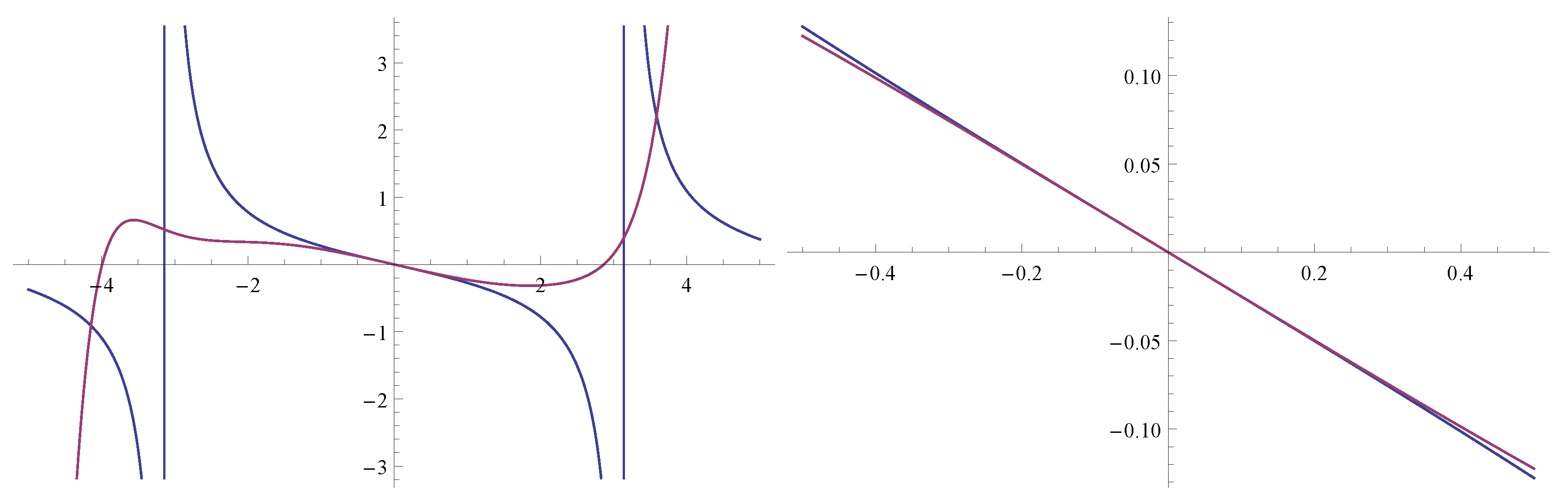
In the following steps, we discuss and investigate the obtained solutions and show their convergence. We applied twelve methods to the fractional nonlinear Duffing equation. We obtained many formulae of exact and approximate solutions:

• In Reference [5], Akbar et al. applied the generalized $(G^{\prime }/G)$-expansion method; here, we also applied an extended model of the $(G^{\prime }/G)$-expansion method. Applying Akbar’s technique permits us to get five various formulae of solutions; our extended method allows us to get three different solutions. Our obtained solutions differ completely from those in Reference [5]. That means we succeeded in obtaining a new formula of solutions for our model.
• Equations (11), (13), (22), (29), (35), (37), (40), and (91) are convergent to each other by equating the parameters in each solution.
• Equations (12), (14), (23), (30), (36), (38), (41), and (92) are convergent to each other by equating the parameters in each solution.
• This convergence of solutions for the fractional nonlinear Duffing equation shows the accuracy of our obtained solutions.
• Table 1 shows the convergence between exact and approximate solutions. The absolute value of error illustrates this convergence.
• Table 1 shows the accuracy of the Adomian decomposition method in the period that is near to zero, like $[-1,1]$.
• According to the solutions that were obtained by the modified Khater method (modified auxiliary equation method) [30], this is considered one of the most general methods in this field, since it covers many of solutions that were obtained by other methods and is also able to obtain more novel and different solutions than other methods.

5. Conclusions

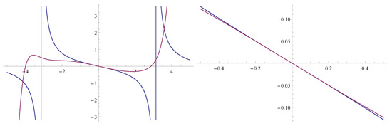
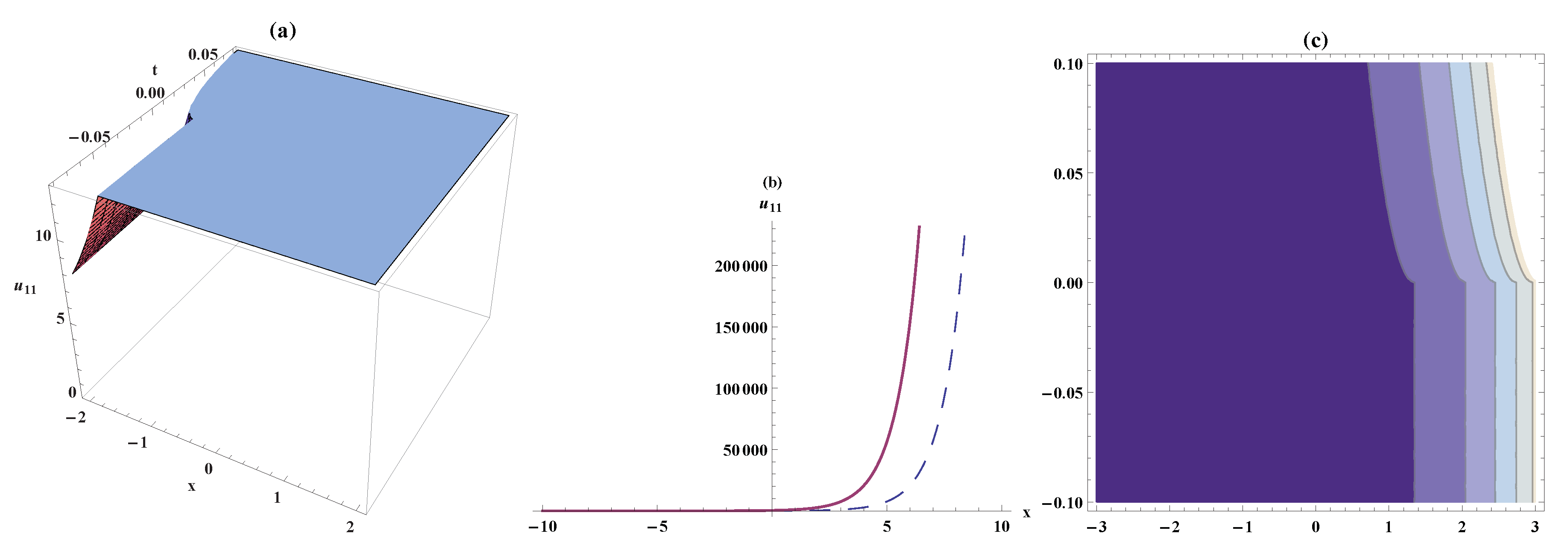
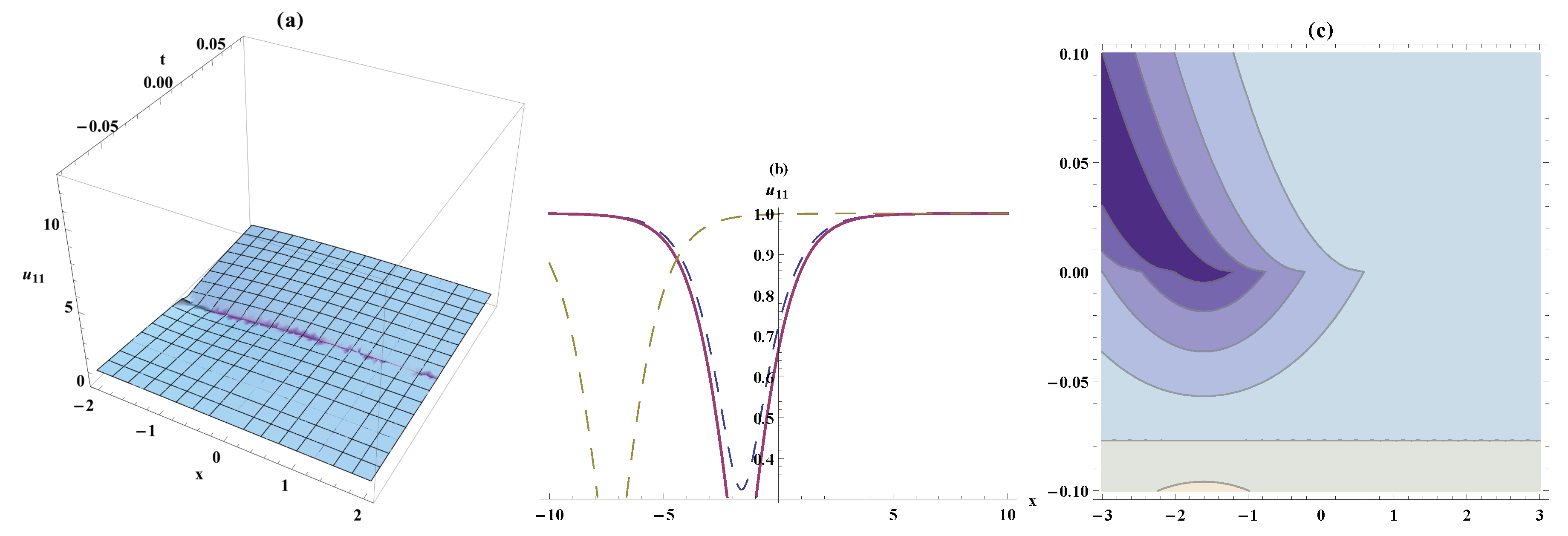
In this paper, we applied eleven recent methods to the nonlinear fractional Duffing equation. We got many various formulas of solutions for this model. We also applied a novel modified method (mKM) that considered the most recent method in this field. The method introduced in Reference [31] was derived in 2017 and after some time, we found the obtained solutions using it were not exact but computational solutions. Here, we applied a novel modified method [30]. We got solitary and approximate solutions for this model. We represented our solutions via making a comparison between them to show the convergence between them. Studying the stability of solutions confirms their ability to be used in many applications. In Figure 1, Figure 2, Figure 3, Figure 4, Figure 5, Figure 6, Figure 7, Figure 8, Figure 9, Figure 10, Figure 11, Figure 12 and Figure 13, we plotted some solutions to investigate more of their properties.

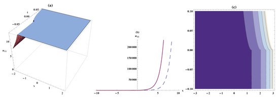
Figure 1. Bright solitary wave, the bistable wave amplitude, and contour plots for Equation (5). On the respective interval $\{x,-2.05,2.05\},\{t,-0.08,0.08\}$, $\{x,-10,10\},\{t,-1,1\}$, $\{x,-3,3\},\{t,-0.1,0.1\}.$

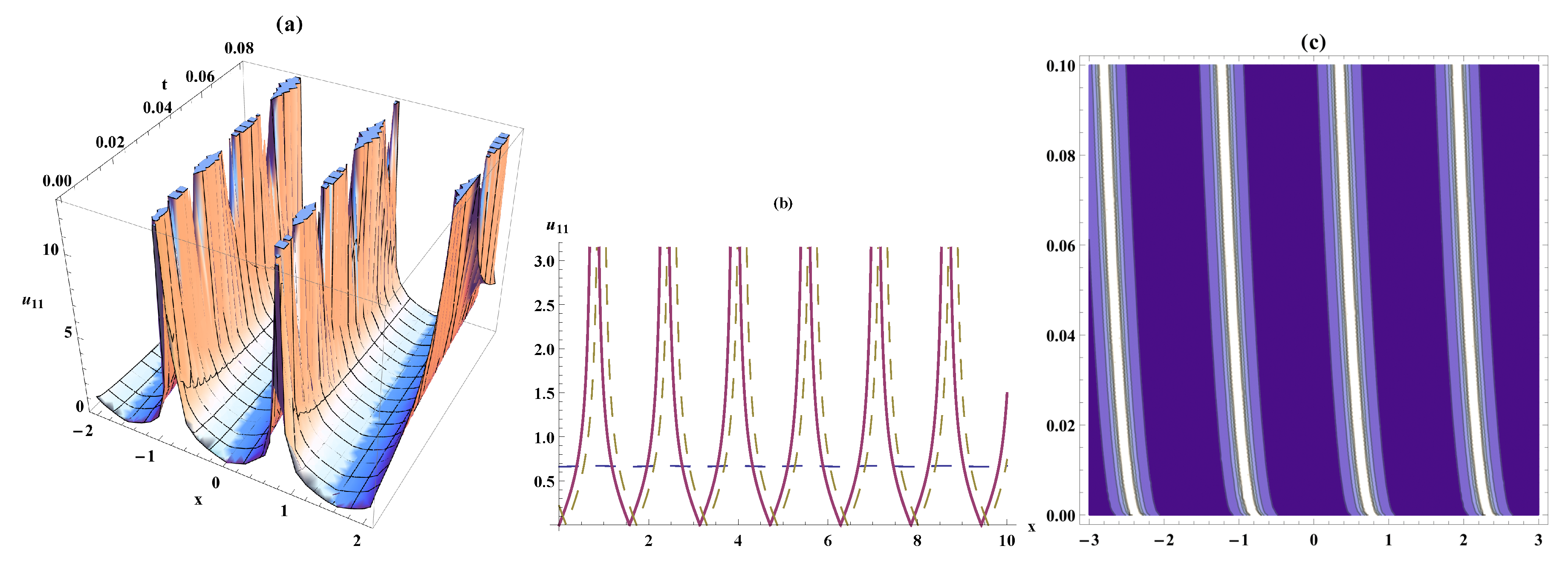
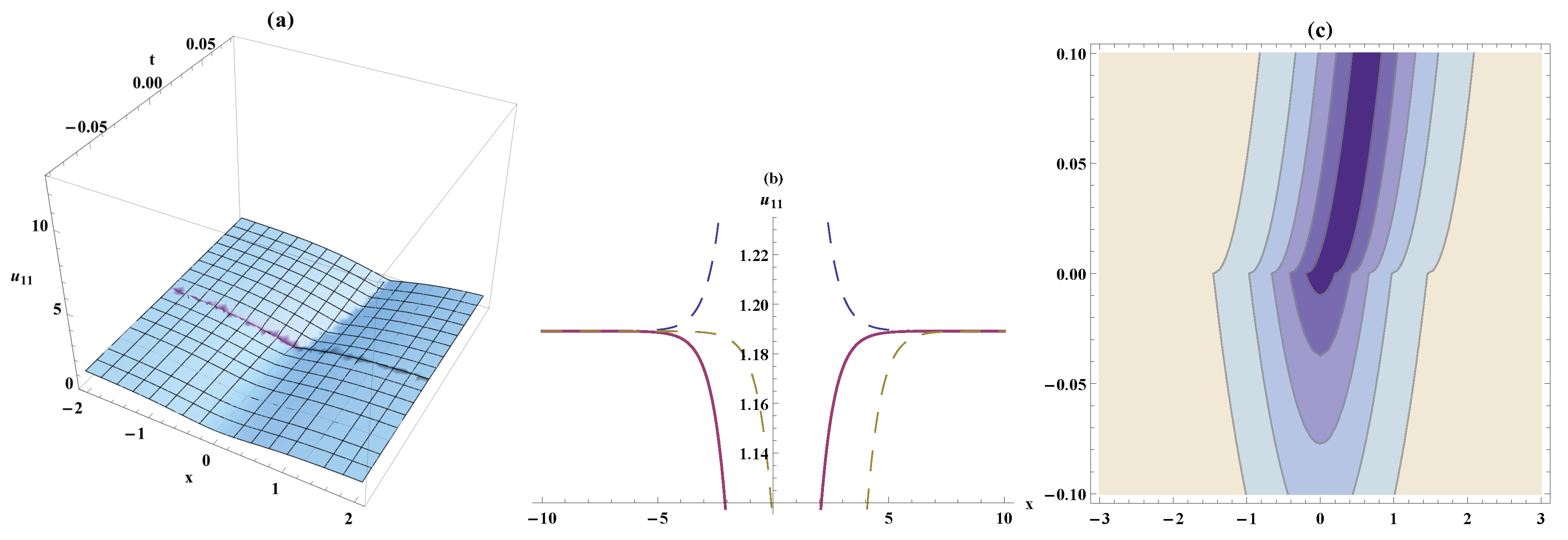
Figure 2. Periodic solitary wave, the bistable wave amplitude, and contour plots for Equation (11). On the respective interval $\{x,-2.05,2.05\},\{t,-0.08,0.08\}$, $\{x,-10,10\},\{t,-1,1\}$, $\{x,-3,3\},\{t,-0.1,0.1\}.$

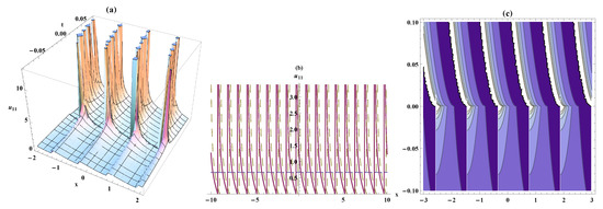
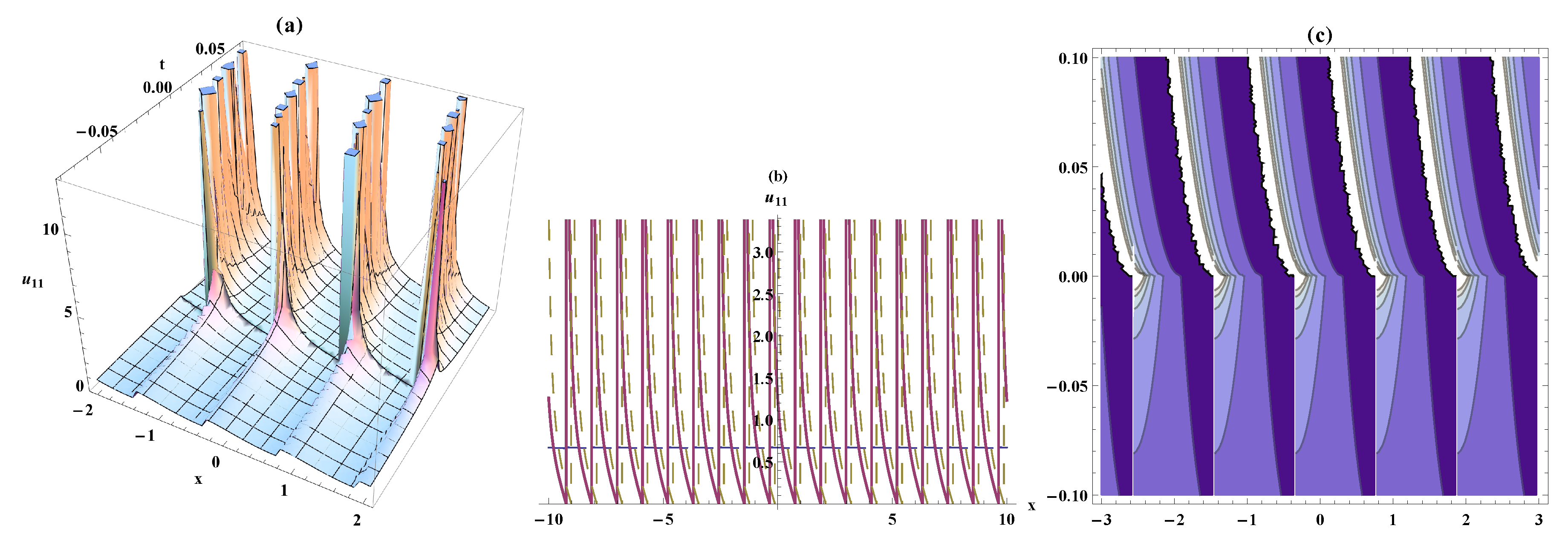
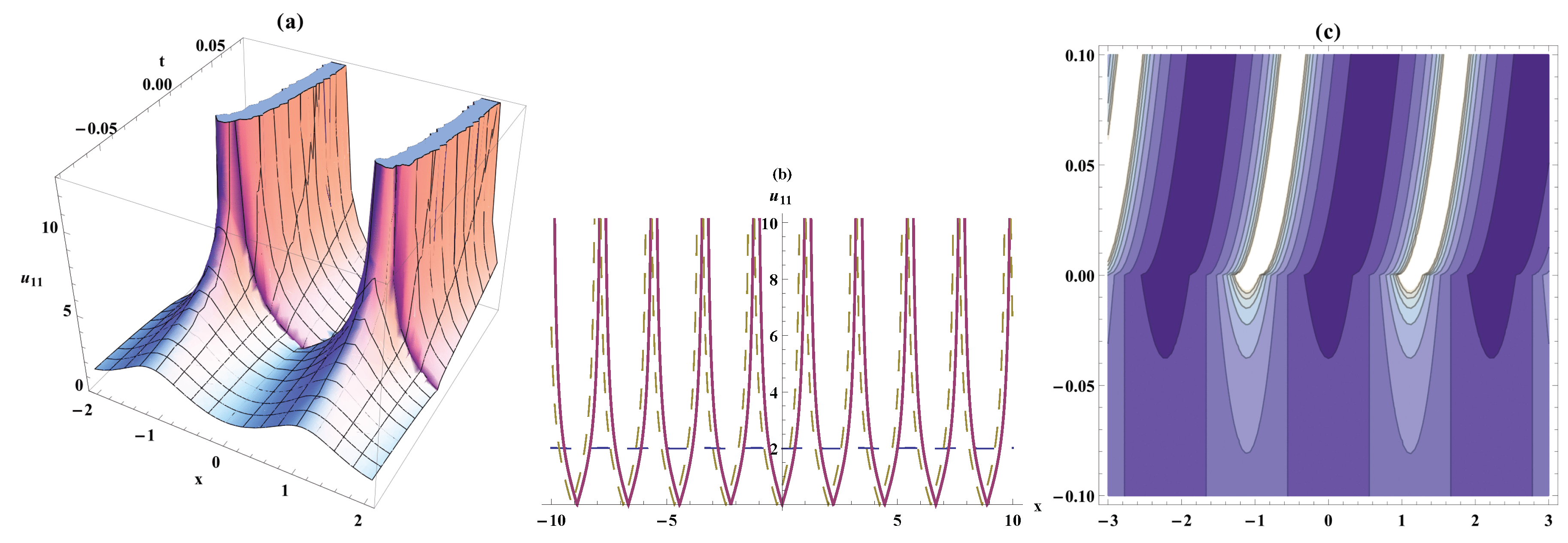
Figure 3. Periodic solitary wave, the bistable wave amplitude, and contour plots for Equation (16). On the respective interval $\{x,-2.05,2.05\},\{t,-0.08,0.08\}$, $\{x,-10,10\},\{t,-1,1\}$, $\{x,-3,3\},\{t,-0.1,0.1\}.$

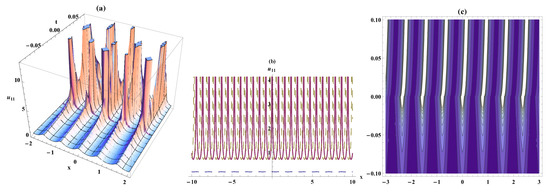
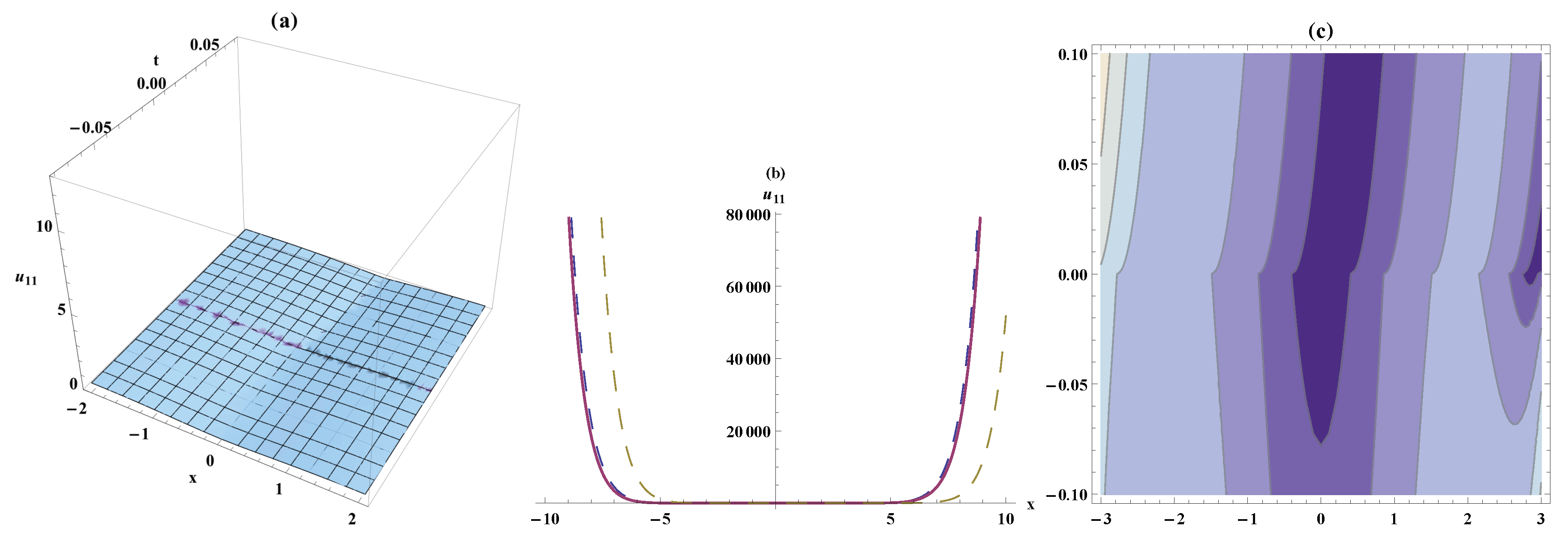
Figure 4. Periodic solitary wave, the bistable wave amplitude and contour plots for Equation (21). On the respectively interval $\{x,-2.05,2.05\},\{t,-0.08,0.08\}$, $\{x,-10,10\},\{t,-1,1\}$, $\{x,-3,3\},\{t,-0.1,0.1\}.$

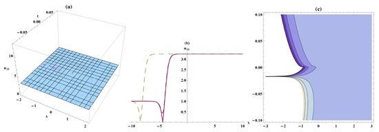
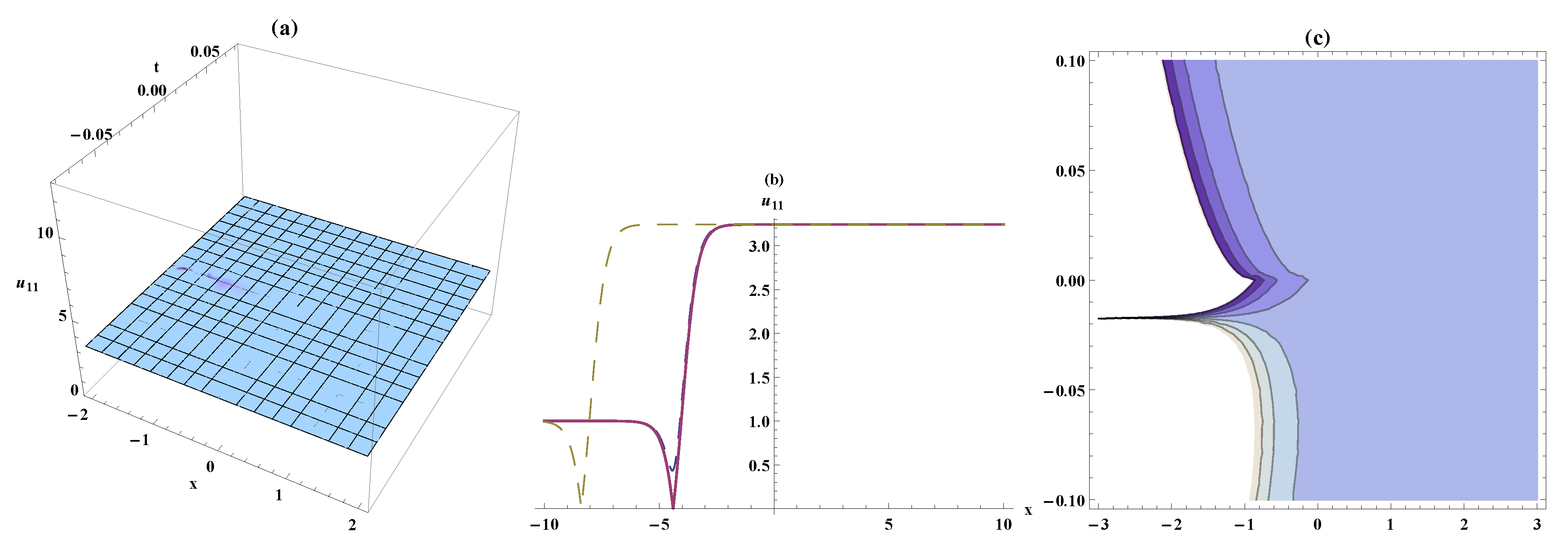
Figure 5. Solitary wave, the bistable wave amplitude, and contour plots for Equation (25). On the respective interval $\{x,-2.05,2.05\},\{t,-0.08,0.08\}$, $\{x,-10,10\},\{t,-1,1\}$, $\{x,-3,3\},\{t,-0.1,0.1\}.$

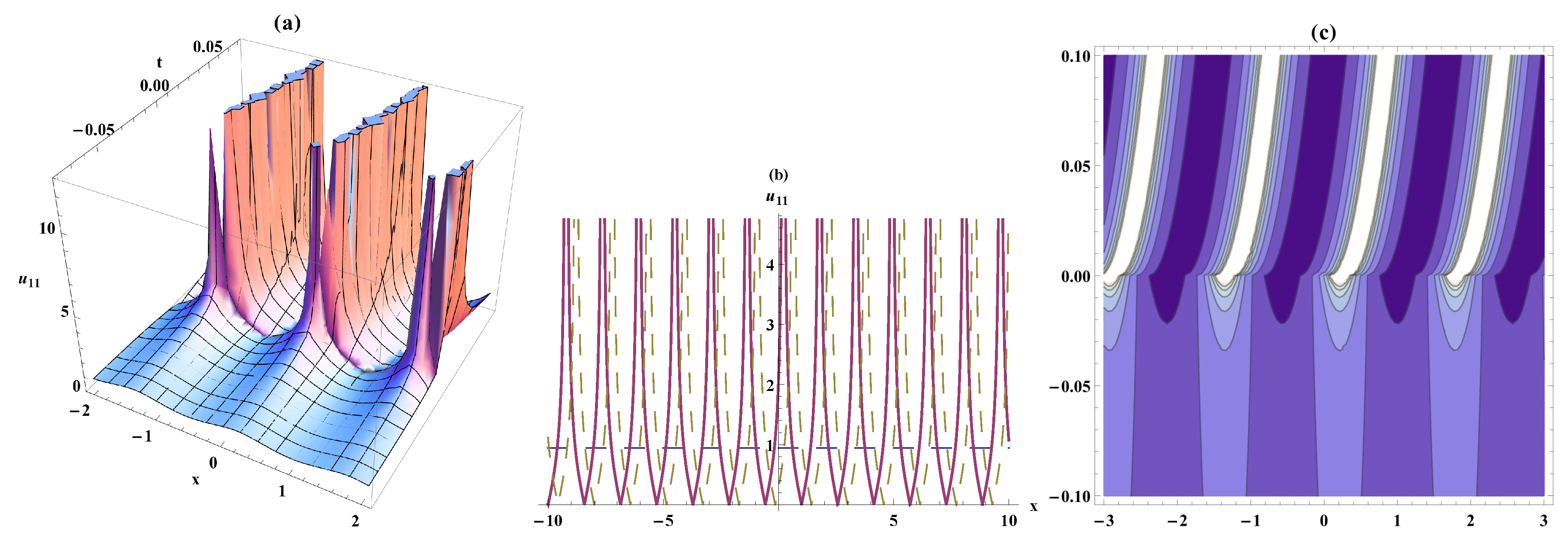
Figure 6. Periodic solitary wave, the bistable wave amplitude, and contour plots for Equation (29). On the respective interval $\{x,-2.05,2.05\},\{t,-0.08,0.08\}$, $\{x,-10,10\},\{t,-1,1\}$, $\{x,-3,3\},\{t,-0.1,0.1\}.$

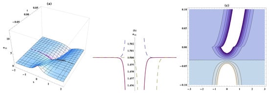
Figure 7. Solitary wave, the bistable wave amplitude, and contour plots for Equation (50). On the respective interval $\{x,-2.05,2.05\},\{t,-0.08,0.08\}$, $\{x,-10,10\},\{t,-1,1\}$, $\{x,-3,3\},\{t,-0.1,0.1\}.$

Figure 8. Solitary wave, the bistable wave amplitude and contour plots for Equation (63). On the respectively interval $\{x,-2.05,2.05\},\{t,-0.08,0.08\}$, $\{x,-10,10\},\{t,-1,1\}$, $\{x,-3,3\},\{t,-0.1,0.1\}.$

Figure 9. Solitary wave, the bistable wave amplitude, and contour plots for Equation (69). On the respective interval $\{x,-2.05,2.05\},\{t,-0.08,0.08\}$, $\{x,-10,10\},\{t,-1,1\}$, $\{x,-3,3\},\{t,-0.1,0.1\}.$

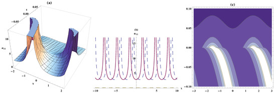
Figure 10. Solitary wave, the bistable wave amplitude, and contour plots for Equation (84). On the respective interval $\{x,-2.05,2.05\},\{t,-0.08,0.08\}$, $\{x,-10,10\},\{t,-1,1\}$, $\{x,-3,3\},\{t,-0.1,0.1\}.$

Figure 11. Solitary wave, the bistable wave amplitude and contour plots for Equation (91). On the respectively interval $\{x,-2.05,2.05\},\{t,-0.08,0.08\}$, $\{x,-10,10\},\{t,-1,1\}$, $\{x,-3,3\},\{t,-0.1,0.1\}.$

Figure 12. Solitary wave, the bistable wave amplitude, and contour plots for Equation (104). On the respective interval $\{x,-2.05,2.05\},\{t,-0.08,0.08\}$, $\{x,-10,10\},\{t,-1,1\}$, $\{x,-3,3\},\{t,-0.1,0.1\}.$

Figure 13. Exact and approximate of Equations (104) and (91) when $\{x,-5,5\}\mathrm{and}\{x,-0.5,0.5\}$.

References

- Kovacic, I.; Brennan, M.J. The Duffing Equation: Nonlinear Oscillators and their Behaviour; John Wiley & Sons: Hoboken, NJ, USA, 2011. [Google Scholar]
- Wang, Y.; An, J.Y. Amplitude-frequency relationship to a fractional Duffing oscillator arising in microphysics and tsunami motion. J. Low Freq. Noise Vib. Act. Control 2018. [Google Scholar] [CrossRef]
- Yusufoǧlu, E. Numerical solution of Duffing equation by the Laplace decomposition algorithm. Appl. Math. Comput. 2006, 177, 572–580. [Google Scholar]
- Daino, B.; Gregori, G.; Wabnitz, S. Stability analysis of nonlinear coherent coupling. J. Appl. Phys. 1985, 58, 4512–4514. [Google Scholar] [CrossRef]
- Akbar, M.A.; Ali, N.H.M.; Roy, R. Closed form solutions of two time fractional nonlinear wave equations. Results Phys. 2018, 9, 1031–1039. [Google Scholar] [CrossRef]
- Zahran, E.H.; Khater, M.M. Modified extended tanh-function method and its applications to the Bogoyavlenskii equation. Appl. Math. Model. 2016, 40, 1769–1775. [Google Scholar] [CrossRef]
- Abdou, M.A. A generalized auxiliary equation method and its applications. Nonlinear Dyn. 2008, 52, 95–102. [Google Scholar] [CrossRef]
- Abdou, M.A. An analytical method for space-time fractional nonlinear differential equations arising in plasma physics. J. Ocean Eng. Sci. 2017, 2, 288–292. [Google Scholar] [CrossRef]
- Abdou, M.A. New periodic solitary wave solutions for a variable-coefficient gardner equation from fluid dynamics and plasma physics. Appl. Math. 2010, 1, 307. [Google Scholar] [CrossRef]
- Abdou, M.A.; Abulwafa, E.M. The Three-wave Method and its Applications. Nonlinear Sci. Lett. A 2010, 1, 373–378. [Google Scholar]
- Abdou, M.A. On the fractional order space-time nonlinear equations arising in plasma physics. Indian J. Phys. 2018, 1–5. [Google Scholar] [CrossRef]
- Abdou, M.A. An analytical approach for space-time fractal order nonlinear dynamics of micro tubules. Waves Random Complex Media 2018, 1–8. [Google Scholar] [CrossRef]
- Biswas, A.; Fessak, M.; Johnson, S.; Beatrice, S.; Milovic, D.; Jovanoski, Z.; Kohl, R.; Majid, F. Optical soliton perturbation in non-Kerr law media: Traveling wave solution. Opt. Laser Technol. 2012, 44, 263–268. [Google Scholar] [CrossRef]
- Khater, M.M.A. Exact traveling wave solutions for the generalized Hirota–Satsuma couple KdV system using the exp (−ϕ(ξ))-expansion method. Cogent Math. 2016, 3, 1172397. [Google Scholar] [CrossRef]
- Rezazadeh, H.; Korkmaz, A.; Eslami, M.; Vahidi, J.; Asghari, R. Traveling wave solution of conformable fractional generalized reaction Duffing model by generalized projective Riccati equation method. Opt. Quantum Electron. 2018, 50, 150. [Google Scholar] [CrossRef]
- Eslami, M.; Rezazadeh, H. The first integral method for Wu-Zhang system with conformable time-fractional derivative. Calcolo 2016, 53, 475–485. [Google Scholar] [CrossRef]
- Eslami, M. Exact traveling wave solutions to the fractional coupled nonlinear Schrödinger equations. Appl. Math. Comput. 2016, 285, 141–148. [Google Scholar] [CrossRef]
- Eslami, M. Trial solution technique to chiral nonlinear Schrödinger’s equation in (1+2)-dimensions. Nonlinear Dyn. 2016, 85, 813–816. [Google Scholar] [CrossRef]
- Attia, R.A.; Lu, D.; Khater, M.M. Structure of New Solitary Solutions for The Schwarzian Korteweg De Varies Equation And (2+1)-Ablowitz–Kaup–Newell–Segur Equation. Phys. J. 2018, 1, 3. [Google Scholar]
- Liu, J.G.; Eslami, M.; Rezazadeh, H.; Mirzazadeh, M. Rational solutions and lump solutions to a non-isospectral and generalized variable-coefficient Kadomtsev–Petviashvili equation. Nonlinear Dyn. 2018, 1–7. [Google Scholar] [CrossRef]
- Wazwaz, A.-M. The tanh method for traveling wave solutions of nonlinear equations. Appl. Math. Comput. 2004, 154, 713–723. [Google Scholar] [CrossRef]
- Liu, J.; Xu, D.; Du, Z. Traveling Wave Solution of a Reaction–Diffusion Predator–Prey System. Qual. Theory Dyn. Syst. 2018, 1–11. [Google Scholar] [CrossRef]
- Taha, W.M.; Aziz, S.I.; Hameed, R.A.; Taha, I.M. New traveling wave solutions of a nonlinear diffusion-convection equation by using standard tanh method. Tikrit J. Pure Sci. 2018, 23, 143–147. [Google Scholar] [CrossRef]
- Khater, M.M.A. The modified simple equation method and its applications in mathematical physics and biology. Glob. J. Sci. Front. Res. F Math. Decis. Sci. 2015, 15, 69–85. [Google Scholar]
- Hosseini, K.; Mayeli, P.; Ansari, R. Modified Kudryashov method for solving the conformable time-fractional Klein-Gordon equations with quadratic and cubic nonlinearities. Opt. Int. J. Light Electron Opt. 2017, 130, 737–742. [Google Scholar] [CrossRef]
- Eslami, M.; Khodadad, F.S.; Nazari, F.; Rezazadeh, H. The first integral method applied to the Bogoyavlenskii equations by means of conformable fractional derivative. Opt. Quantum Electron. 2017, 49, 391. [Google Scholar] [CrossRef]
- Zhao, D.; Luo, M. General conformable fractional derivative and its physical interpretation. Calcolo 2017, 54, 903–917. [Google Scholar] [CrossRef]
- Ilie, M.; Biazar, J.; Ayati, Z. General solution of Bernoulli and Riccati fractional differential equations based on conformable fractional derivative. Int. J. Appl. Math. Res. 2017, 6, 49–51. [Google Scholar]
- Mozaffari, F.S.; Hassanabadi, H.; Sobhani, H.; Chung, W.S. Investigation of the Dirac Equation by Using the Conformable Fractional Derivative. J. Korean Phys. Soc. 2018, 72, 987–990. [Google Scholar] [CrossRef]
- Khater, M.; Attia, R.; Lu, D. Modified Auxiliary Equation Method versus Three Nonlinear Fractional Biological Models in Present Explicit Wave Solutions. Math. Comput. Appl. 2019, 24, 1. [Google Scholar] [CrossRef]
- Bibi, S.; Mohyud-Din, S.T.; Khan, U.; Ahmed, N. Khater method for nonlinear Sharma Tasso-Olever (STO) equation of fractional order. Results Phys. 2017, 7, 4440–4450. [Google Scholar] [CrossRef]
© 2019 by the authors. Licensee MDPI, Basel, Switzerland. This article is an open access article distributed under the terms and conditions of the Creative Commons Attribution (CC BY) license (http://creativecommons.org/licenses/by/4.0/).