Optimal Strategies for Psoriasis Treatment

Abstract

Within a given time interval we consider a nonlinear system of differential equations describing psoriasis treatment. Its phase variables define the concentrations of T-lymphocytes, keratinocytes and dendritic cells. Two scalar bounded controls are introduced into this system to reflect medication dosages aimed at suppressing interactions between T-lymphocytes and keratinocytes, and between T-lymphocytes and dendritic cells. For such a controlled system, a minimization problem of the concentration of keratinocytes at the terminal time is considered. For its analysis, the Pontryagin maximum principle is applied. As a result of this analysis, the properties of the optimal controls and their possible types are established. It is shown that each of these controls is either a bang-bang type on the entire time interval or (in addition to bang-bang type) contains a singular arc. The obtained analytical results are confirmed by numerical calculations using the software “BOCOP-2.0.5”. Their detailed analysis and the corresponding conclusions are presented.

1. Introduction

Psoriasis is an immune-mediated inflammatory skin disease that affects 2–3% of the population around the world [1]. The most characteristic features of the pathology are hyperproliferation and disrupted epidermal differentiation, altered immunological and vascular skin profiles. Manifestations of psoriasis can vary according to severity: from weak, when only a few characteristic psoriatic plaques are present on the body of patients, to extremely severe ones, when the lesion affects almost the entire surface of the body and joints. Disease can significantly reduce the standard of living and performance of patients [2]. There are established links between psoriasis and other diseases: obesity, diabetes, cardiovascular diseases, metabolic syndrome, and depression [3]. Molecular-genetic causes of the disease are still not fully established. At the same time, various polymorphisms associated with psoriasis as well as several environmental factors that can lead to the manifestation of this disease are identified [4]. To date, about 150 million people around the world are suffering from psoriasis. In the USA the annual cost of treatment is about $\$12$ billion, while the existing therapies can only relieve symptoms and increase remission time. In addition, recent studies have revealed the division of psoriasis into subtypes, depending on which patients may respond differently to therapy. In some cases, despite costly and prolonged treatment, the patient’s condition may not improve [5]. In recent years, studies have greatly expanded the understanding of the pathogenesis of psoriasis and allowed the development of numerous therapies.

In psoriasis, mathematical models are effectively used to predict cellular behavior of the skin in both normal and pathological conditions. Among all possible models [6], we highlight the models that are described by systems of differential equations [6,7,8,9,10,11,12,13,14,15]. In turn, controlled mathematical models are used to simulate the use of medication and dosage regimen, compare the effects of various drugs on the affected areas of the skin, and to determine the most effective methods of treatment. Within the framework of a specific model, optimal control theory is used to find the best strategies in one sense or another for psoriasis treatment.

For mathematical models of psoriasis treatment, optimal control problems were considered in [15,16,17], where the optimal treatment strategies minimizing the weighted sum of the total concentration of keratinocytes and the total cost of the treatment were found numerically. This cost of psoriasis treatment was expressed by an integral of the square of control, and these models were described using systems of differential equations linear in control. After applying the Pontryagin maximum principle as a necessary optimality condition, the corresponding optimal control problems were reduced to two-point boundary value problems for the maximum principle, which were then solved numerically, applying standard mathematical software. This was because the right-hand sides of the systems of differential equations of such boundary value problems were Lipschitz functions of the phase and adjoint variables.

In the optimal control problems for mathematical models of diseases and the spread of epidemics, the total cost of treatment can also be expressed by an integral of control [18,19,20,21]. In this case, the models are still described by systems of differential equations that are linear in control. Then, as shown in [21,22], after applying the Pontryagin maximum principle to such problems, the corresponding optimal controls can contain singular arcs on which these controls are not uniquely determined from the maximum condition. After the existence of such singular arcs are established on appropriate singular intervals, the corresponding optimality conditions are checked, and the concatenations of singular and nonsingular intervals are found, the finding of specific optimal solutions in optimal control problems is still performed only numerically. This paper shows that optimal controls can contain singular arcs in the minimization problem for the mathematical model of psoriasis treatment even in the absence of the controls in the integral terms of the functional to be minimized responsible for the cost of this treatment.

This paper is organized as follows. Section 2 is devoted to the description of the mathematical model of psoriasis treatment and the formulation of the corresponding optimal control problem for it. Namely, we consider a nonlinear controlled system of three differential equations that presents the process of treating this disease. Its phase variables determine the concentrations of T-lymphocytes, keratinocytes, and dendritic cells. The interaction of these types of cells leads to the appearance and development of psoriasis. There are two scalar bounded controls in the system that reflect all types of psoriasis treatment: skin creams that prevent or inhibit the formation, development and spread of psoriatic skin lesions, as well as pills and injections, also aimed at achieving similar results. At the same time, skin creams suppress the interaction between T-lymphocytes and keratinocytes; pills and injections weaken the interaction between T-lymphocytes and dendritic cells. All such medications are aimed at achieving the main goal, which is to reduce the number of keratinocytes. Therefore, for such a controlled system, at a given time interval the problem of minimizing the concentration of keratinocytes at the end of the time interval is stated. An optimal solution for such a problem, consisting of the optimal controls and the corresponding optimal solutions of the system, is analyzed using the Pontryagin maximum principle. Its application to the considered minimization problem is discussed in Section 3. Here, also possible types of the optimal controls are discussed: whether they are only bang-bang functions, or they can contain singular arcs in addition to the bang-bang intervals. A detailed analysis of the behavior of the optimal controls is given in Section 4. Here, we study the properties of the corresponding switching functions, which are crucial in such analysis. Using the Lie brackets of the geometric control theory allows us to obtain the Cauchy problem for the switching functions. Such a Cauchy problem makes it possible to draw the conclusions about possible singular arcs of the optimal controls. The first one shows that these controls do not simultaneously have singular arcs on the same singular intervals. The second of them is that when one optimal control has a singular arc on some singular interval, the second optimal control is constant on this interval and takes one of its boundary values. The next two sections, Section 5 and Section 6, are devoted to a detailed analysis of singular arcs of each optimal control. In these sections it is shown that one of them can have a singular arc of the order of two, and the other can contain a singular arc of order one. Also, for each of these singular arcs the corresponding necessary optimality conditions are checked (Kelly-Cope-Moyer condition and Kelly condition). Finally, the forms of concatenations of the singular arcs of the optimal controls with nonsingular intervals on which such controls are bang-bang functions are considered. Since, as previously mentioned, after discussing all such issues, finding the specific optimal solutions is carried out numerically, then in Section 7 the results of the corresponding numerical calculations and their discussion are presented. Section 8 contains our conclusions.

2. Mathematical Model and Optimal Control Problem

Let a time interval $[0,T]$ be given, which is the period of psoriasis treatment. We consider on this interval a mathematical model that establishes the links between the concentrations $l(t)$, $k(t)$, $m(t)$ of T-lymphocytes, keratinocytes, and dendritic cells, respectively, because interactions between these types of cells cause a disease such as psoriasis. Such a model is the nonlinear system of differential equations:

$$\left\{\begin{array}{c}{l}^{\prime }(t)=\sigma -\delta v(t)l(t)m(t)-{\gamma }_{1}u(t)l(t)k(t)-\mu l(t),\hfill \\ k^{\prime }(t)=(\beta +\delta )v(t)l(t)m(t)+{\gamma }_{2}u(t)l(t)k(t)-\lambda k(t),\hfill \\ m^{\prime }(t)=\rho -\beta v(t)l(t)m(t)-\nu m(t),\hfill \end{array}\right.$$

(1)

with given initial values:

$$l(0)=l_0,k(0)=k_0,m(0)=m_0;l_0,m_0,k_0>0.$$

(2)

In System (1) we suppose that $\sigma$ is the constant rate of accumulation for T-lymphocytes and $\rho$ is the constant accumulation rate of dendritic cells. The rate of activation of T-lymphocytes by dendritic cells is $\delta$ and $\beta$ is the activation rate of dendritic cells by T-lymphocytes. Also, we consider that the removal rates of T-lymphocytes, keratinocytes and dendritic cells are denoted by $\mu$, $\lambda$ and $\nu$, respectively. Finally, we suppose that ${\gamma }_1$ is the rate of activation of keratinocytes by T-lymphocytes and growth of keratinocytes due to T-lymphocytes occurs at the rate ${\gamma }_2$.

Next, in System (1) two control functions $u(t)$ and $v(t)$ are introduced. The control $u(t)$ is at the places of interaction between T-lymphocytes and keratinocytes and reflects the medication dosage to restrict the excessive growth of keratinocytes. In a similar way, the control $v(t)$ is at the places of interaction between T-lymphocytes and dendritic cells and reflects the medication dosage for the restriction of the excessive growth of keratinocytes as well. The controls $u(t)$ and $v(t)$ subject to the following restrictions:

$$0<u_{min}\le u(t)\le 1,0<v_{min}\le v(t)\le 1.$$

(3)

We consider that the set of all admissible controls $\Omega (T)$ is formed by all possible pairs of Lebesgue measurable functions $(u(t),v(t))$, which for almost all $t\in [0,T]$ satisfy Inequality (3).

Let us introduce a region:

$$\Lambda =\left\{{(l,k,m)}^{\top }\in {\mathrm{R}}^3:l>0,k>0,m>0,l+k+m<M\right\},$$

where M is a positive constant that depends on the parameters $\sigma$, $\rho$, $\beta$, $\delta$, $\mu$, $\lambda$, $\nu$, ${\gamma }_1$, ${\gamma }_2$ of System (1) and its initial values $l_0$, $k_0$, $m_0$ from (2). Here ${\mathrm{R}}^3$ is the Euclidean space consisting of all column vectors and the sign ${}^{\top }$ means transposition.

Then, the boundedness, positiveness, and continuation of the solutions for System (1) is stated by the following lemma.

Lemma 1.

Let the inclusion ${(l_0,k_0,m_0)}^{\top }\in \Lambda$ be valid. Then, for any pair of admissible controls $(u(t),v(t))$ the corresponding absolutely continuous solutions $l(t)$, $k(t)$, $m(t)$ for System (1) are defined on the entire interval $[0,T]$ and satisfy the inclusion:

$${(l(t),k(t),m(t))}^{\top }\in \Lambda ,t\in (0,T].$$

(4)

Remark 1.

Relationship (4) implies that the region Λ is a positive invariant set for System (1). The proof of Lemma 1 is fairly straightforward, and we omit it. Proofs of such statements are given, for example, in [16,23,24].

Now, let us consider for System (1) on the set of admissible controls $\Omega (T)$ the following minimization problem:

$$J(u(·),v(·))=k(T)\to \underset{(u(·),v(·))\in \Omega (T)}{min},$$

(5)

which consists in minimizing the concentration of keratinocites at the final moment T of psoriasis treatment. As already noted in [25], the optimal control problem (5) differs from problems that are typically considered in the literature on the control of psoriasis models [15,16,17,26] in that the functional from (5) does not include an integral of the weighted sum of the squares of the controls $u(t)$ and $v(t)$, which is responsible for the total cost of drug dosages. In psoriasis treatment, in most cases, either a skin cream, or an oral medication are used. Both prescribed medications have regular daily dosage and are not as harmful for patients as the drugs used in chemotherapy for cancer treatment [21]. Therefore, the total cost of psoriasis treatment in the meaning “harm” to a patient and that usually mathematically is described by an integral of the weighted sum of the squares of the controls, can be ignored. Moreover, using the terminal functional from (5) instead of corresponding integral functional [15,16,17,26] simplifies the subsequent analytical arguments.

The existence in the minimization problem (5) of the optimal controls $(u_{*}(t),v_{*}(t))$ and the corresponding optimal solutions $l_{*}(t)$, $k_{*}(t)$, $m_{*}(t)$ for System (1) follows from Lemma 1 and Theorem 4 ([27], Chapter 4).

Finally, based on the results from [17,23,26], we assume that the following assumption is true.

Assumption 1.

Let the inequalities:

$${\gamma }_1\ne {\gamma }_2,(\beta +\delta ){\gamma }_1>\delta {\gamma }_2,\lambda >\mu ,\lambda >\nu$$

(6)

be valid.

Let us introduce the constants:

$$\alpha ={\gamma }_1{\gamma }_2^{-1}(\beta +\delta )-\delta ,ϵ=\alpha (\lambda -\nu )+\delta (\lambda -\mu ).$$

By this assumption, it is easy to see that these constants are positive.

3. Pontryagin Maximum Principle

We apply the Pontryagin maximum principle [28] to analyze the optimal controls $u_{*}(t)$, $v_{*}(t)$ and the corresponding optimal solutions $l_{*}(t)$, $k_{*}(t)$, $m_{*}(t)$. Firstly, let us define the Hamiltonian:

$$\begin{array}{cc}\hfill H(l,m,k,u,v,& {\psi }_1,{\psi }_2,{\psi }_3)=(\sigma -\delta vlm-{\gamma }_{1}ulk-\mu l){\psi }_1\hfill \\ & +((\beta +\delta )vlm+{\gamma }_{2}ulk-\lambda k){\psi }_2+(\rho -\beta vlm-\nu m){\psi }_3,\hfill \end{array}$$

where ${\psi }_1$, ${\psi }_2$, ${\psi }_3$ are the adjoint variables.

Secondly, we calculate the required partial derivatives:

$$\begin{array}{cc}\hfill H_l^{\prime }(l,m,k,u,v,{\psi }_1,{\psi }_2,{\psi }_3)& =uk({\gamma }_2{\psi }_2-{\gamma }_1{\psi }_1)\hfill \\ & +vm(-\delta {\psi }_1+(\beta +\delta ){\psi }_2-\beta {\psi }_3)-\mu {\psi }_1,\hfill \\ \hfill H_k^{\prime }(l,m,k,u,v,{\psi }_1,{\psi }_2,{\psi }_3)& =ul({\gamma }_2{\psi }_2-{\gamma }_1{\psi }_1)-\lambda {\psi }_2,\hfill \\ \hfill H_m^{\prime }(l,m,k,u,v,{\psi }_1,{\psi }_2,{\psi }_3)& =vl(-\delta {\psi }_1+(\beta +\delta ){\psi }_2-\beta {\psi }_3)-\nu {\psi }_3,\hfill \\ \hfill H_u^{\prime }(l,m,k,u,v,{\psi }_1,{\psi }_2,{\psi }_3)& =lk({\gamma }_2{\psi }_2-{\gamma }_1{\psi }_1),\hfill \\ \hfill H_v^{\prime }(l,m,k,u,v,{\psi }_1,{\psi }_2,{\psi }_3)& =lm(-\delta {\psi }_1+(\beta +\delta ){\psi }_2-\beta {\psi }_3).\hfill \end{array}$$

Then, in accordance with the Pontryagin maximum principle, for the optimal controls $u_{*}(t)$, $v_{*}(t)$ and the optimal solutions $l_{*}(t)$, $k_{*}(t)$, $m_{*}(t)$ there exists a vector-function ${\psi }_{*}(t)={({\psi }_1^{*}(t),{\psi }_2^{*}(t),{\psi }_3^{*}(t))}^{\top }$ such that:

• ${\psi }_{*}(t)$ is a nontrivial solution of the adjoint system:

  $$\left\{\begin{array}{c}{{\psi }_1^{*}}^{\prime }(t)=-u_{*}(t)k_{*}(t)({\gamma }_2{\psi }_2^{*}(t)-{\gamma }_1{\psi }_1^{*}(t))\hfill \\ -v_{*}(t)m_{*}(t)(-\delta {\psi }_1^{*}(t)+(\beta +\delta ){\psi }_2^{*}(t)-\beta {\psi }_3^{*}(t))+\mu {\psi }_1^{*}(t),\hfill \\ {{\psi }_2^{*}}^{\prime }(t)=-u_{*}(t)l_{*}(t)({\gamma }_2{\psi }_2^{*}(t)-{\gamma }_1{\psi }_1^{*}(t))+\lambda {\psi }_2^{*}(t),\hfill \\ {{\psi }_3^{*}}^{\prime }(t)=-v_{*}(t)l_{*}(t)(-\delta {\psi }_1^{*}(t)+(\beta +\delta ){\psi }_2^{*}(t)-\beta {\psi }_3^{*}(t))+\nu {\psi }_3^{*}(t),\hfill \\ {\psi }_1^{*}(T)=0,{\psi }_2^{*}(T)=-1,{\psi }_3^{*}(T)=0;\hfill \end{array}\right.$$

  (7)
• the controls $u_{*}(t)$ and $v_{*}(t)$ maximize the Hamiltonian

  $$H(l_{*}(t),k_{*}(t),m_{*}(t),u,v,{\psi }_1^{*}(t),{\psi }_2^{*}(t),{\psi }_3^{*}(t))$$

  with respect to variables $u\in [u_{min},1]$ and $v\in [v_{min},1]$ for almost all $t\in [0,T]$, and therefore they satisfy the relationships:

  $$u_{*}(t)=\left\{\begin{array}{cc}1\hfill & ,\mathrm{if}{L}_u(t)>0,\hfill \\ \mathrm{any}u\in [u_{min},1]\hfill & ,\mathrm{if}{L}_u(t)=0,\hfill \\ u_{min}\hfill & ,\mathrm{if}{L}_u(t)<0;\hfill \end{array}\right.$$

  (8)

  $$v_{*}(t)=\left\{\begin{array}{cc}1\hfill & ,\mathrm{if}{L}_v(t)>0,\hfill \\ \mathrm{any}v\in [v_{min},1]\hfill & ,\mathrm{if}{L}_v(t)=0,\hfill \\ v_{min}\hfill & ,\mathrm{if}{L}_v(t)<0;\hfill \end{array}\right.$$

  (9)

  where the functions:

  $$\begin{array}{c}{L}_u(t)=l_{*}(t)k_{*}(t)({\gamma }_2{\psi }_2^{*}(t)-{\gamma }_1{\psi }_1^{*}(t)),\hfill \\ L_v(t)=l_{*}(t)m_{*}(t)(-\delta {\psi }_1^{*}(t)+(\beta +\delta ){\psi }_2^{*}(t)-\beta {\psi }_3^{*}(t))\hfill \end{array}$$

  (10)

  are the switching functions describing the behavior of the controls $u_{*}(t)$ and $v_{*}(t)$ in accordance with Formulas (8) and (9), respectively.

Analysis of Formulas (8) and (9) shows possible types of the optimal controls $u_{*}(t)$ and $v_{*}(t)$. They can only have a bang-bang type and switch between the corresponding values $u_{min}$ and 1, $v_{min}$ and 1. This occurs, when passing through the points at which the switching functions $L_u(t)$ and $L_v(t)$ are zero, the sign of these functions changes. Or, in addition to intervals of a bang-bang type, the controls $u_{*}(t)$ and $v_{*}(t)$ can also contain singular arcs [22,29]. This occurs when the switching functions $L_u(t)$ and $L_v(t)$ individually or both simultaneously vanish identically on certain subintervals of the interval $[0,T]$. Furthermore, such subintervals we will call as singular intervals. The following sections are devoted to a detailed study of singular arcs for the optimal controls $u_{*}(t)$ and $v_{*}(t)$.

Now, we establish the important property of the controls $u_{*}(t)$ and $v_{*}(t)$. Namely, by Lemma 1, the initial values of System (7), Formula (10), and the continuity of the switching functions $L_u(t)$ and $L_v(t)$, the following lemma is valid.

Lemma 2.

There exist such values $t_{★}^u,t_{★}^v\in [0,T)$ that the inequalities $L_u(t)<0$ and $L_v(t)<0$ hold for all t from the corresponding intervals $(t_{★}^u,T]$ and $(t_{★}^v,T]$.

Corollary 1.

Lemma 2 and Formulas (8) and (9) imply the following relationships for the optimal controls $u_{*}(t)$ and $v_{*}(t)$:

$$u_{*}(t)=u_{min},t\in (t_{★}^u,T];v_{*}(t)=v_{min},t\in (t_{★}^v,T].$$

4. Differential Equations of the Switching Functions

Let us obtain differential equations for the switching functions $L_u(t)$ and $L_v(t)$. To do this, we draw on the concepts and notations of geometric control theory from [21,22].

Again, we consider the Euclidean space ${\mathrm{R}}^3$ in which the value $⟨\tau ,s⟩$ is the scalar product of its elements. Let $z={(l,k,m)}^{\top }\in {\mathrm{R}}^3$. Then, we rewrite System (1) as follows

$$z^{\prime }(t)=f(z(t))+u(t)g(z(t))+v(t)h(z(t)),$$

(11)

where

$$f(z)=\left(\begin{array}{c}\sigma -\mu l\\ -\lambda k\\ \rho -\nu m\end{array}\right),g(z)=\left(\begin{array}{c}-{\gamma }_{1}lk\\ {\gamma }_{2}lk\\ 0\end{array}\right),h(z)=\left(\begin{array}{c}-\delta lm\\ (\beta +\delta )lm\\ -\beta lm\end{array}\right)$$

(12)

with $f(z)$ the drift and $g(z)$, $h(z)$ the control vector fields of this system. Here $z(t)$ is the column vector consisting of the solutions $l(t)$, $k(t)$, $m(t)$ that correspond to the admissible controls $u(t)$ and $v(t)$, that is $z(t)={(l(t),k(t),m(t))}^{\top }\in {\mathrm{R}}^3$. Let $Df(z)$, $Dg(z)$ and $Dh(z)$ be the Jacobian matrices of the vector functions $f(z)$, $g(z)$ and $h(z)$, respectively. By Formula (12), we find the following relationships:

$$\begin{array}{c}Df(z)=\left(\begin{array}{ccc}-\mu & 0& 0\\ 0& -\lambda & 0\\ 0& 0& -\nu \end{array}\right),Dg(z)=\left(\begin{array}{ccc}-{\gamma }_{1}k& -{\gamma }_{1}l& 0\\ {\gamma }_{2}k& {\gamma }_{2}l& 0\\ 0& 0& 0\end{array}\right),\hfill \\ Dh(z)=\left(\begin{array}{ccc}-\delta m& 0& -\delta l\\ (\beta +\delta )m& 0& (\beta +\delta )l\\ -\beta m& 0& -\beta l\end{array}\right).\hfill \end{array}$$

(13)

Then, using the introduced concepts and notations, it is easy to see that $z_{*}(t)={(l_{*}(t),k_{*}(t),m_{*}(t))}^{\top }$ is the optimal trajectory for System (11) corresponding to the optimal controls $u_{*}(t)$ and $v_{*}(t)$; ${\psi }_{*}(t)={({\psi }_1^{*}(t),{\psi }_2^{*}(t),{\psi }_3^{*}(t))}^{\top }$ is the appropriate nontrivial solution for the adjoint System (7), or in the new notations:

$$\left\{\begin{array}{c}{\psi }_{*}^{\prime }(t)=-{\left(Df(z_{*}(t))+u_{*}(t)Dg(z_{*}(t)+v_{*}(t)Dh(z_{*}(t))\right)}^{\top }{\psi }_{*}(t),\hfill \\ {\psi }_{*}(T)={(0,-1,0)}^{\top }.\hfill \end{array}\right.$$

(14)

The Hamiltonian

$$H(t)=H(l_{*}(t),k_{*}(t),m_{*}(t),u_{*}(t),v_{*}(t),{\psi }_1^{*}(t),{\psi }_2^{*}(t),{\psi }_3^{*}(t))$$

takes the form:

$$H(t)=⟨{\psi }_{*}(t),f(z_{*}(t))⟩+u_{*}(t)⟨{\psi }_{*}(t),g(z_{*}(t))⟩+v_{*}(t)⟨{\psi }_{*}(t),h(z_{*}(t))⟩.$$

The switching functions $L_u(t)$ and $L_v(t)$, defined by Formula (10), become the scalar products of the adjoint function ${\psi }_{*}(t)$ with the corresponding control fields $g(z_{*}(t))$ and $h(z_{*}(t))$:

$$L_u(t)=⟨{\psi }_{*}(t),g(z_{*}(t))⟩,L_v(t)=⟨{\psi }_{*}(t),h(z_{*}(t))⟩.$$

(15)

Now, according to [21,22], we introduce for the drift and control vector fields $f(z)$, $g(z)$ and $h(z)$ the corresponding Lie brackets:

$$[f,g](z)=Dg(z)f(z)-Df(z)g(z),$$

(16)

$$[f,h](z)=Dh(z)f(z)-Df(z)h(z),$$

(17)

$$[g,h](z)=Dh(z)g(z)-Dg(z)h(z).$$

(18)

Using (11) and (14)–(18), the derivatives of the switching functions $L_u(t)$ and $L_v(t)$ can be obtained as follows

$$L_u^{\prime }(t)=⟨{\psi }_{*}(t),[f,g](z_{*}(t))⟩+v_{*}(t)⟨{\psi }_{*}(t),[h,g](z_{*}(t))⟩,$$

(19)

$$L_v^{\prime }(t)=⟨{\psi }_{*}(t),[f,h](z_{*}(t))⟩+u_{*}(t)⟨{\psi }_{*}(t),[g,h](z_{*}(t))⟩.$$

(20)

Now, using (12) and (13) in (16)–(18), we compute the Lie brackets $[f,g](z)$, $[f,h](z)$ and $[g,h](z)$. As a result, we find the formulas:

$$\begin{array}{c}[f,g](z)=\left(\begin{array}{c}-{\gamma }_{1}k(\sigma -\lambda l)\\ {\gamma }_{2}k(\sigma -\mu l)\\ 0\end{array}\right),[g,h](z)=\left(\begin{array}{c}{\gamma }_1(\beta +\delta )l^{2}m\\ -{\gamma }_2(\beta +\delta )l^{2}m-\alpha {\gamma }_{2}lkm\\ {\gamma }_1\beta lkm\end{array}\right),\hfill \\ [f,h](z)=\left(\begin{array}{c}-\delta ((\rho l+\sigma m)-\nu lm)\\ (\beta +\delta )((\rho l+\sigma m)+(\lambda -\mu -\nu )lm)\\ -\beta ((\rho l+\sigma m)-\mu lm)\end{array}\right).\hfill \end{array}$$

(21)

Let us write these Lie brackets in a more convenient form for the subsequent analysis. For this, we introduce the following linearly independent vectors:

$$p=\left(\begin{array}{c}-{\gamma }_1\\ {\gamma }_2\\ 0\end{array}\right),q=\left(\begin{array}{c}-\delta \\ \beta +\delta \\ -\beta \end{array}\right),r=\left(\begin{array}{c}1\\ 0\\ 0\end{array}\right).$$

It is easy to see that the following representations for the control vector fields $g(z)$ and $h(z)$ are valid:

$$g(z)=lk·p,h(z)=lm·q.$$

Using these relationships, Formula (15) for the switching functions $L_u(t)$ and $L_v(t)$ can be rewritten as

$$L_u(t)=l_{*}(t)k_{*}(t)⟨{\psi }_{*}(t),p⟩,L_v(t)=l_{*}(t)m_{*}(t)⟨{\psi }_{*}(t),q⟩.$$

(22)

Now, let us find the decompositions of the Lie brackets $[f,g](z)$, $[f,h](z)$ and $[g,h](z)$, defined by (21), by the vectors p, q, r. As a result, we have the representations:

$$[f,g](z)=k(\sigma -\mu l)·p+{\gamma }_1(\lambda -\mu )lk·r,$$

(23)

$$[f,h](z)={\gamma }_2^{-1}(\beta +\delta )(\lambda -\nu )lm·p+(\rho l+\sigma m-\mu lm)·q+ϵlm·r,$$

(24)

$$[g,h](z)=-lm((\beta +\delta )l-\delta k)·p-{\gamma }_{1}lkm·q.$$

(25)

Next, let us introduce the auxiliary function $G(t)=⟨{\psi }_{*}(t),r⟩={\psi }_1^{*}(t)$, and define the following absolutely continuous functions:

$$\begin{array}{cc}\hfill a_u(t)& =l_{*}^{-1}(t)(\sigma -\mu l_{*}(t)),a_v(t)={\gamma }_2^{-1}(\beta +\delta )(\lambda -\nu )k_{*}^{-1}(t)m_{*}(t),\hfill \\ \hfill b_v(t)& =l_{*}^{-1}(t)m_{*}^{-1}(t)(\rho l_{*}(t)+\sigma m_{*}(t)-\mu l_{*}(t)m_{*}(t)),\hfill \\ \hfill c_u(t)& ={\gamma }_1(\lambda -\mu )l_{*}(t)k_{*}(t),c_v(t)=ϵl_{*}(t)m_{*}(t),\hfill \\ \hfill d(t)& =k_{*}^{-1}(t)m_{*}(t)((\beta +\delta )l_{*}(t)-\delta k_{*}(t)),e(t)={\gamma }_1{k}_{*}(t).\hfill \end{array}$$

(26)

It is easy to see that the functions $c_u(t)$ and $c_v(t)$ are positive on the interval $[0,T]$.

Finally, substituting (23)–(25) into (19), (20) and using (22), (26), we find the required differential equations for the switching functions $L_u(t)$ and $L_v(t)$:

$$\begin{array}{cc}\hfill L_u^{\prime }(t)& =a_u(t)L_u(t)+c_u(t)G(t)+v_{*}(t)(d(t)L_u(t)+e(t)L_v(t)),\hfill \\ \hfill L_v^{\prime }(t)& =a_v(t)L_u(t)+b_v(t)L_v(t)+c_v(t)G(t)\hfill \\ & -u_{*}(t)(d(t)L_u(t)+e(t)L_v(t)).\hfill \end{array}$$

We add to these equations the first equation of System (7), written with use of the functions $L_u(t)$, $L_v(t)$, $G(t)$:

$$G^{\prime }(t)=-u_{*}(t)l_{*}^{-1}(t)L_u(t)-v_{*}(t)l_{*}^{-1}(t)L_v(t)+\mu G(t),$$

as well as the corresponding initial values:

$$L_u(T)=-{\gamma }_2{l}_{*}(T)k_{*}(T),L_v(T)=-(\beta +\delta )l_{*}(T)m_{*}(T),G(T)=0.$$

As a result, we obtain the Cauchy problem for the switching functions $L_u(t)$, $L_v(t)$ and the function $G(t)$:

$$\left\{\begin{array}{c}{L}_u^{\prime }(t)=a_u(t)L_u(t)+c_u(t)G(t)+v_{*}(t)(d(t)L_u(t)+e(t)L_v(t)),\hfill \\ L_v^{\prime }(t)=a_v(t)L_u(t)+b_v(t)L_v(t)+c_v(t)G(t)\hfill \\ -u_{*}(t)(d(t)L_u(t)+e(t)L_v(t)),\hfill \\ G^{\prime }(t)=-u_{*}(t)l_{*}^{-1}(t)L_u(t)-v_{*}(t)l_{*}^{-1}(t)L_v(t)+\mu G(t),\hfill \\ L_u(T)=-{\gamma }_2{l}_{*}(T)k_{*}(T),L_v(T)=-(\beta +\delta )l_{*}(T)m_{*}(T),G(T)=0,\hfill \end{array}\right.$$

(27)

which we will use to justify the properties of the functions $L_u(t)$ and $L_v(t)$.

Now, let us establish the properties of the switching functions $L_u(t)$ and $L_v(t)$. Firstly, the following lemma is true.

Lemma 3.

There is no subinterval of the interval $[0,T]$ at which both switching functions $L_u(t)$ and $L_v(t)$ are identically zero.

Proof of Lemma 3.

We suppose the contrary. Let there be the interval ${\Delta }_{u,v}\subset [0,T]$ on which the functions $L_u(t)$ and $L_v(t)$ identically equal to zero. Then, their derivatives $L_u^{\prime }(t)$ and $L_v^{\prime }(t)$ almost everywhere on this subinterval also vanish. From the first two differential equations of the Cauchy problem (27) we find that $G(t)=0$ everywhere on the subinterval ${\Delta }_{u,v}$. Hence, on this subinterval the derivative $G^{\prime }(t)$ is almost everywhere zero. Therefore, the third differential equation of the Cauchy problem (27) is also satisfied. Using the definition of the function $G(t)$, Lemma 1 and Formula (10), we find that the adjoint function ${\psi }_{*}(t)$ vanishes identically on the subinterval ${\Delta }_{u,v}$. Since the system of linear differential equations (7) is homogeneous, then ${\psi }_{*}(t)=0$ identically everywhere on the interval $[0,T]$, which is contradictory. Hence, our assumption was wrong, and the subinterval ${\Delta }_{u,v}\subset [0,T]$ on which both switching functions $L_u(t)$ and $L_v(t)$ are identically zero, does not exist. This completes the proof. ☐

Secondly, the following lemma holds.

Lemma 4.

Let the subinterval ${\Delta }_u\subset [0,T]$ be a singular interval of the optimal control $u_{*}(t)$. Then, everywhere on this subinterval, the optimal control $v_{*}(t)$ is constant and takes one of the values $\{v_{min};1\}$.

Proof of Lemma 4.

On the subinterval ${\Delta }_u$ the switching function $L_u(t)$ is identically zero, and its derivative $L_u^{\prime }(t)$ vanishes almost everywhere on this interval. Then, the first differential equation of the Cauchy problem (27) yields the equality:

$$c_u(t)G(t)+v_{*}(t)e(t)L_v(t)=0,t\in {\Delta }_u.$$

(28)

Let us suppose that the switching function $L_v(t)$ is zero at some point $t_0^u\in {\Delta }_u$, that is

$$L_v(t_0^u)=0.$$

(29)

Then, (28) implies the equality:

$$G(t_0^u)=0.$$

(30)

The identical equality to zero of the function $L_u(t)$ on the subinterval ${\Delta }_u$ and (29), (30) lead us to the equality ${\psi }_{*}(t_0^u)=0$. A further repetition of the corresponding arguments from Lemma 3 gives a contradiction. Hence, our assumption was wrong, and the switching function $L_v(t)$ does not vanish at any point of the subinterval ${\Delta }_u$. Therefore, it is sign-definite on this subinterval, and, by Formula (9), the optimal control $v_{*}(t)$ corresponding to it, is constant and takes one of the values $\{v_{min};1\}$. This completes the proof. ☐

Furthermore, performing arguments similar to the arguments of Lemma 4, one can show that the following lemma is valid.

Lemma 5.

Let the subinterval ${\Delta }_v\subset [0,T]$ be a singular interval of the optimal control $v_{*}(t)$. Then, everywhere on this subinterval, the optimal control $u_{*}(t)$ is constant and takes one of the values $\{u_{min};1\}$.

Now, we strengthen the result obtained in Lemma 4. Namely, the following lemma holds.

Lemma 6.

Let the subinterval ${\Delta }_u=(t_1^u,t_2^u)\subset [0,T]$, where $t_1^u>0$, be a singular interval of the optimal control $u_{*}(t)$. Then, there exists a number ${\epsilon }_u>0$ such that on the interval $(t_1^u-{ϵ}_u,t_2^u+{ϵ}_u)$ the optimal control $v_{*}(t)$ is constant and takes one of the values $\{v_{min};1\}$.

Proof of Lemma 6.

It suffices to show that the ends of the subinterval ${\Delta }_u=(t_1^u,t_2^u)$ cannot be zeros of the switching function $L_v(t)$, which is an absolutely continuous function. Indeed, if such a fact holds, that is the inequalities:

$$L_v(t_1^u)\ne 0,L_v(t_2^u)\ne 0$$

are true, then Lemma 6 immediately follows from the Theorem on the stability of the sign of a continuous function [30]. Therefore, for definiteness, we consider the right end $t_2^u$ of the subinterval ${\Delta }_u$. Let us suppose the contrary. This means that the equality:

$$L_v(t_2^u)=0$$

(31)

is valid. Then, for the function $G(t)$ the following two cases are possible.

Case 1. Let $G(t_2^u)=0$. The definition of the function $G(t)$, Lemma 1 and the second formula of (10) imply the relationship:

$$(\beta +\delta ){\psi }_2^{*}(t_2^u)=\beta {\psi }_3^{*}(t_2^u).$$

(32)

If ${\psi }_2^{*}(t_2^u)=0$, then (32) yields ${\psi }_3^{*}(t_2^u)=0$. This fact leads to contradictory equality ${\psi }_{*}(t_2^u)=0$, as the proofs of Lemmas 3 and 4 show. If ${\psi }_2^{*}(t_2^u)\ne 0$, then again the definition of the function $G(t)$, Lemma 1 and the first formula of (10) imply $L_u(t_2^u)\ne 0$. The absolutely continuity of the function $L_u(t)$ and the Theorem on the stability of the sign of a continuous function [30] lead to the existence of a left neighborhood of the point $t_2^u$ at which the switching function $L_u(t)$ is sign-definite. This contradicts the fact that such a left neighborhood of the point $t_2^u$ belongs to the subinterval ${\Delta }_u$, which is a singular portion of the optimal control $u_{*}(t)$. Thus, Case 1 is impossible.

Case 2. Let $G(t_2^u)\ne 0$. For definiteness, we consider that the inequality:

$$G(t_2^u)>0$$

(33)

is true. As it was already noted, $L_v(t)$ and $G(t)$ are the absolutely continuous functions. In Lemma 4 it was established that the control $v_{*}(t)$ is constant on the subinterval ${\Delta }_u$, that is $v_{*}(t)=v_{*}$. Therefore, by (31), (33) and the Theorem on the stability of the sign of a continuous function [30], there exists the interval $({\tilde{t}}_2^u,t_2^u)\subset {\Delta }_u$ on which the inequality:

$$c_u(t)G(t)+v_{*}e(t)L_v(t)>0$$

(34)

is valid. Let ${\tilde{t}}_0^u$ be the midpoint of this interval. We rewrite the first differential equation from the Cauchy problem (27) as

$$L_u^{\prime }(t)=(a_u(t)+v_{*}d(t))L_u(t)+(c_u(t)G(t)+v_{*}e(t)L_v(t)).$$

Then, we integrate this equation on the interval $({\tilde{t}}_2^u,t_2^u)$ with the initial value $L_u({\tilde{t}}_0^u)=0$. As a result, the following formula can be found:

$$L_u(t)=\underset{{\tilde{t}}_0^u}{\overset{t}{\int }}{\mathrm{e}}^{\underset{s}{\overset{t}{\int }}(a_u(\xi )+v_{*}d(\xi ))d\xi }\left(c_u(s)G(s)+v_{*}e(s)L_v(s)\right)ds.$$

(35)

By (34) and (35), we obtain the positivity of the function $L_u(t)$ for $t>{\tilde{t}}_0^u$ and the negativity of this function for $t<{\tilde{t}}_0^u$ on the interval $({\tilde{t}}_2^u,t_2^u)$. This is again contradictory. Hence, Case 2 is also impossible.

Thus, our assumption was wrong, and the switching function $L_v(t)$ does not vanish at the point $t_2^u$. This completes the proof. ☐

Furthermore, carrying out arguments similar to the arguments of Lemma 6, we can show that the following lemma holds, which strengthens the result of Lemma 5.

Lemma 7.

Let the subinterval ${\Delta }_v=(t_1^v,t_2^v)\subset [0,T]$, where $t_1^v>0$, be a singular interval of the optimal control $v_{*}(t)$. Then, there exists a number ${\epsilon }_v>0$ such that on the interval $(t_1^v-{ϵ}_v,t_2^v+{ϵ}_v)$ the optimal control $u_{*}(t)$ is constant and takes one of the values $\{u_{min};1\}$.

Remark 2.

From Lemmas 4–7 we conclude that when a singular arc occurs for one of the optimal controls, $u_{*}(t)$ or $v_{*}(t)$, System (1) becomes on the corresponding singular interval a system with one control, because the other control is constant.

Next, in Section 5 and Section 6, we separately study the existence of singular arcs of the optimal controls $u_{*}(t)$ and $v_{*}(t)$, applying the approach from [21]. It consists in the sequential differentiation on a singular interval of the corresponding switching function. We carry out this differentiation if the derivative of even order does not have a nonzero term containing control. If such a term appears in a second order derivative, then we say that a singular arc is of the order of one. If it occurs in a derivative of the fourth order, then it is considered that the singular arc is of the order of two. Then, the corresponding optimality condition of a singular arc is checked. If it is satisfied, we find the formulas of the optimal control and the corresponding optimal solutions of System (1) on a singular interval corresponding to such a singular arc. Also, the type of concatenation of this singular arc with non-singular intervals is studied, where the considered optimal control is bang-bang. Finally, we demonstrate a singular arc of the optimal control through the results of a numerical solution of the minimization problem (5), presented in Section 7.

5. Investigation of a Singular Arc of the Optimal Control ${\mathit{u}}_{\mathbf{*}}\mathbf{(}\mathit{t}\mathbf{)}$

Let us study the existence of a singular arc of the optimal control $u_{*}(t)$. According to [22,29], this means the existence of a subinterval ${\Delta }_u\subset [0,T]$ on which the corresponding switching function $L_u(t)$ identically vanishes. By Lemma 4, everywhere on this subinterval the optimal control $v_{*}(t)$ is a constant function taking one of the values $\{v_{min};1\}$, that is,

$$v_{*}(t)=v_{*}\in \{v_{min};1\},t\in {\Delta }_u.$$

Then, Formula (19) of the first derivative $L_u^{(1)}(t)$ of the switching function $L_u(t)$ is rewritten in the form:

$$L_u^{(1)}(t)=⟨{\psi }_{*}(t),[f+v_{*}h,g](z_{*}(t))⟩,t\in {\Delta }_u.$$

(36)

Let us transform the right-hand side of this formula. To do this, we rewrite (23) and (25) as

$$[f,g](z)={\theta }_{f,g}(z)p+{\chi }_{f,g}(z)r,[h,g](z)={\theta }_{h,g}(z)p+{\eta }_{h,g}(z)q,$$

(37)

where

$$\begin{array}{cc}\hfill {\theta }_{f,g}(z)& =(\sigma -\mu l)k,{\chi }_{f,g}(z)={\gamma }_1(\lambda -\mu )lk,\hfill \\ \hfill {\theta }_{h,g}(z)& =lm((\beta +\delta )l-\delta k),{\eta }_{h,g}(z)={\gamma }_{1}lkm.\hfill \end{array}$$

Then, using (37), we can write the Lie bracket $[f+v_{*}h,g](z)$ as follows

$$[f+v_{*}h,g](z)={\theta }_u(z)p+{\eta }_u(z)q+{\chi }_u(z)r,$$

(38)

where

$$\begin{array}{cc}\hfill {\theta }_u(z)& ={\theta }_{f,g}(z)+v_{*}{\theta }_{h,g}(z)=(\sigma -\mu l)k+v_{*}lm((\beta +\delta )l-\delta k),\hfill \\ \hfill {\eta }_u(z)& =v_{*}{\eta }_{h,g}(z)={\gamma }_1{v}_{*}lkm,\hfill \\ \hfill {\chi }_u(z)& ={\chi }_{f,g}(z)={\gamma }_1(\lambda -\mu )lk.\hfill \end{array}$$

Substituting (38) into the right-hand side of (36), we obtain the relationship:

$$L_u^{(1)}(t)={\theta }_u(z_{*}(t))⟨{\psi }_{*}(t),p⟩+{\eta }_u(z_{*}(t))⟨{\psi }_{*}(t),q⟩+{\chi }_u(z_{*}(t))⟨{\psi }_{*}(t),r⟩,t\in {\Delta }_u.$$

(39)

Now, differentiating (36), we find the formula for the second derivative $L_u^{(2)}(t)$ of the switching function $L_u(t)$:

$$\begin{array}{cc}\hfill L_u^{(2)}(t)& =⟨{\psi }_{*}(t),[f+v_{*}h,[f+v_{*}h,g]](z_{*}(t))⟩\hfill \\ & +u_{*}(t)⟨{\psi }_{*}(t),[g,[f+v_{*}h,g]](z_{*}(t))⟩,t\in {\Delta }_u.\hfill \end{array}$$

(40)

Let us transform the terms of this formula. First, we consider the second term and its factor

$$⟨{\psi }_{*}(t),[g,[f+v_{*}h,g]](z_{*}(t))⟩.$$

(41)

By analogy with (16)–(18), we have equality:

$$[g,[f+v_{*}h,g]](z)=D[f+v_{*}h,g](z)g(z)-Dg(z)[f+v_{*}h,g](z),$$

(42)

where $D[f+v_{*}h,g](z)$ is the Jacobi matrix of the vector function $[f+v_{*}h,g](z)$. Using (38), we find the relationship:

$$\begin{array}{cc}\hfill D[f+v_{*}h,g](z)& =D({\theta }_u(z)p)+D({\eta }_u(z)q)+D({\chi }_u(z)r)\hfill \\ & =p{(\nabla {\theta }_u(z))}^{\top }+q{(\nabla {\eta }_u(z))}^{\top }+r{(\nabla {\chi }_u(z))}^{\top },\hfill \end{array}$$

(43)

where $\nabla {\theta }_u(z)$, $\nabla {\eta }_u(z)$, $\nabla {\chi }_u(z)$ are the column gradients of the functions ${\theta }_u(z)$, ${\eta }_u(z)$, ${\chi }_u(z)$, respectively. In addition, the representations:

$$Dg(z)=p{({\tau }_g(z))}^{\top },Dh(z)=q{({\tau }_h(z))}^{\top }$$

(44)

are valid, where the vector functions ${\tau }_g(z)$, ${\tau }_h(z)$ are defined as

$${\tau }_g(z)=\left(\begin{array}{c}k\\ l\\ 0\end{array}\right),{\tau }_h(z)=\left(\begin{array}{c}m\\ 0\\ l\end{array}\right).$$

We substitute (43) and the first representation of (44) into (42). After the necessary transformations, the following relationship can be obtained:

$$\begin{array}{c}[g,[f+v_{*}h,g]](z)=\left(⟨\nabla {\theta }_u(z),g(z)⟩-⟨[f+v_{*}h,g](z),{\tau }_g(z)⟩\right)p\hfill \\ +⟨\nabla {\eta }_u(z),g(z)⟩q+⟨\nabla {\chi }_u(z),g(z)⟩r.\hfill \end{array}$$

Substituting this expression into (41), we find the formula:

$$\begin{array}{cc}\hfill ⟨{\psi }_{*}(t),[g,& [f+v_{*}h,g]](z_{*}(t))⟩\hfill \\ & =(⟨\nabla {\theta }_u(z_{*}(t)),g(z_{*}(t))⟩-⟨[f+v_{*}h,g](z_{*}(t)),{\tau }_g(z_{*}(t))⟩)⟨{\psi }_{*}(t),p⟩\hfill \\ & +⟨\nabla {\eta }_u(z_{*}(t)),g(z_{*}(t))⟩⟨{\psi }_{*}(t),q⟩+⟨\nabla {\chi }_u(z_{*}(t)),g(z_{*}(t))⟩⟨{\psi }_{*}(t),r⟩.\hfill \end{array}$$

(45)

In (39) the function ${\chi }_u(z_{*}(t))$ is positive on the interval $[0,T]$. Therefore, let us express the scalar product $⟨{\psi }_{*}(t),r⟩$ through the remaining terms as follows

$$\begin{array}{cc}\hfill ⟨{\psi }_{*}(t),r⟩& ={\chi }_u^{-1}(z_{*}(t))L_u^{(1)}(t)-{\chi }_u^{-1}(z_{*}(t)){\theta }_u(z_{*}(t))⟨{\psi }_{*}(t),p⟩\hfill \\ & -{\chi }_u^{-1}(z_{*}(t)){\eta }_u(z_{*}(t))⟨{\psi }_{*}(t),q⟩,\hfill \end{array}$$

(46)

and then, we substitute this expression into (45). After the necessary transformations, the following relationship finally can be obtained:

$$\begin{array}{cc}\hfill ⟨{\psi }_{*}(t)& ,[g,[f+v_{*}h,g]](z_{*}(t))⟩={\chi }_u^{-1}(z_{*}(t))⟨\nabla {\chi }_u(z_{*}(t)),g(z_{*}(t))⟩L_u^{(1)}(t)\hfill \\ & +{\chi }_u^{-1}(z_{*}(t))\{⟨{\chi }_u(z_{*}(t))\nabla {\theta }_u(z_{*}(t))-{\theta }_u(z_{*}(t))\nabla {\chi }_u(z_{*}(t)),g(z_{*}(t))⟩\hfill \\ & -{\chi }_u(z_{*}(t))⟨[f+v_{*}h,g](z_{*}(t)),{\tau }_g(z_{*}(t))⟩\}⟨{\psi }_{*}(t),p⟩\hfill \\ & +{\chi }_u^{-1}(z_{*}(t))⟨{\chi }_u(z_{*}(t))\nabla {\eta }_u(z_{*}(t))-{\eta }_u(z_{*}(t))\nabla {\chi }_u(z_{*}(t)),g(z_{*}(t))⟩⟨{\psi }_{*}(t),q⟩.\hfill \end{array}$$

(47)

On the subinterval ${\Delta }_u$ the switching function $L_u(t)$ vanishes identically, that is

$$L_u(t)=l_{*}(t)k_{*}(t)⟨{\psi }_{*}(t),p⟩=0,$$

(48)

and therefore its first derivative $L_u^{(1)}(t)$ is also zero everywhere on this subinterval:

$$L_u^{(1)}(t)=0.$$

(49)

Then, Formula (47) is simplified and takes the following form:

$$\begin{array}{cc}\hfill ⟨{\psi }_{*}(t)& ,[g,[f+v_{*}h,g]](z_{*}(t))⟩\hfill \\ & ={\chi }_u^{-1}(z_{*}(t))⟨{\chi }_u(z_{*}(t))\nabla {\eta }_u(z_{*}(t))-{\eta }_u(z_{*}(t))\nabla {\chi }_u(z_{*}(t)),g(z_{*}(t))⟩⟨{\psi }_{*}(t),q⟩.\hfill \end{array}$$

(50)

Let us calculate the right-hand side of this formula. For this, we consider the expression $({\chi }_u(z)\nabla {\eta }_u(z)-{\eta }_u(z)\nabla {\chi }_u(z))$. Calculating the column gradients $\nabla {\eta }_u(z)$, $\nabla {\chi }_u(z)$ of the corresponding functions ${\eta }_u(z)$, ${\chi }_u(z)$, the following equality can be found:

$${\chi }_u(z)\nabla {\eta }_u(z)-{\eta }_u(z)\nabla {\chi }_u(z)={\gamma }_1(\lambda -\mu )v_{*}\left(\begin{array}{c}0\\ 0\\ l^2{k}^2\end{array}\right).$$

(51)

Multiplying this expression scalarly by the vector function $g(z)$ from (12), we conclude that the scalar product

$$⟨{\chi }_u(z)\nabla {\eta }_u(z)-{\eta }_u(z)\nabla {\chi }_u(z),g(z)⟩$$

is zero. Consequently, (50) has the form:

$$⟨{\psi }_{*}(t),[g,[f+v_{*}h,g]](z_{*}(t))⟩=0,t\in {\Delta }_u.$$

(52)

Now, let us consider the first term on the right-hand side of (40):

$$⟨{\psi }_{*}(t),[f+v_{*}h,[f+v_{*}h,g]](z_{*}(t))⟩.$$

(53)

By analogy with (42), we have the equality:

$$[f+v_{*}h,[f+v_{*}h,g]](z)=D[f+v_{*}h,g](z)(f+v_{*}h)(z)-D(f+v_{*}h)(z)[f+v_{*}h,g](z).$$

(54)

Let us find the Jacobi matrix $D(f+v_{*}h)(z)$. The Jacobi matrix $Dh(z)$ of the vector function $h(z)$ is given by the second formula of (44). The use of direct calculations allows us to find the representation of the Jacobi matrix $Df(z)$ from (13) in the following form:

$$Df(z)=p{\left(\begin{array}{c}0\\ -{\gamma }_2^{-1}\lambda \\ -{\gamma }_2^{-1}{\beta }^{-1}(\beta +\delta )\nu \end{array}\right)}^{\top }+q{\left(\begin{array}{c}0\\ 0\\ {\beta }^{-1}\nu \end{array}\right)}^{\top }+r{\left(\begin{array}{c}-\mu \\ -{\gamma }_1{\gamma }_2^{-1}\lambda \\ -{\beta }^{-1}\alpha \nu \end{array}\right)}^{\top }.$$

(55)

Then, we obtain the required representation of the Jacobi matrix $D(f+v_{*}h)(z)$ as

$$D(f+v_{*}h)(z)=p{({\tau }_p^u)}^{\top }+q{({\tau }_q^u(z))}^{\top }+r{({\tau }_r^u)}^{\top },$$

(56)

where

$${\tau }_p^u=\left(\begin{array}{c}0\\ -{\gamma }_2^{-1}\lambda \\ -{\gamma }_2^{-1}{\beta }^{-1}(\beta +\delta )\nu \end{array}\right),{\tau }_q^u(z)=\left(\begin{array}{c}{v}_{*}m\\ 0\\ {\beta }^{-1}\nu +v_{*}l\end{array}\right),{\tau }_r^u=\left(\begin{array}{c}-\mu \\ -{\gamma }_1{\gamma }_2^{-1}\lambda \\ -{\beta }^{-1}\alpha \nu \end{array}\right).$$

We substitute (43) and (56) into (54). After the necessary transformations, the following formula can be found:

$$\begin{array}{c}[f+v_{*}h,[f+v_{*}h,g]](z)=\left(⟨\nabla {\theta }_u(z),(f+v_{*}h)(z)⟩-⟨[f+v_{*}h,g](z),{\tau }_p^u⟩\right)p\hfill \\ +\left(⟨\nabla {\eta }_u(z),(f+v_{*}h)(z)⟩-⟨[f+v_{*}h,g](z),{\tau }_q^u(z)⟩\right)q\hfill \\ +\left(⟨\nabla {\chi }_u(z),(f+v_{*}h)(z)⟩-⟨[f+v_{*}h,g](z),{\tau }_r^u⟩\right)r.\hfill \end{array}$$

Substituting this formula into (53), we obtain the expression:

$$\begin{array}{cc}\hfill ⟨{\psi }_{*}(t)& ,[f+v_{*}h,[f+v_{*}h,g]](z_{*}(t))⟩\hfill \\ & =\left(⟨\nabla {\theta }_u(z_{*}(t)),(f+v_{*}h)(z_{*}(t))⟩-⟨[f+v_{*}h,g](z_{*}(t)),{\tau }_p^u⟩\right)⟨{\psi }_{*}(t),p⟩\hfill \\ & +\left(⟨\nabla {\eta }_u(z_{*}(t)),(f+v_{*}h)(z_{*}(t))⟩-⟨[f+v_{*}h,g](z_{*}(t)),{\tau }_q^u(z_{*}(t))⟩\right)⟨{\psi }_{*}(t),q⟩\hfill \\ & +\left(⟨\nabla {\chi }_u(z_{*}(t)),(f+v_{*}h)(z_{*}(t))⟩-⟨[f+v_{*}h,g](z_{*}(t)),{\tau }_r^u⟩\right)⟨{\psi }_{*}(t),r⟩.\hfill \end{array}$$

(57)

Finally, let us substitute (46) into (57). After the necessary transformations, we find the relationship:

$$\begin{array}{c}⟨{\psi }_{*}(t),[f+v_{*}h,[f+v_{*}h,g]](z_{*}(t))⟩\hfill \\ ={\chi }_u^{-1}(z_{*}(t))\left\{⟨\nabla {\chi }_u(z_{*}(t)),(f+v_{*}h)(z_{*}(t))⟩-⟨[f+v_{*}h,g](z_{*}(t)),{\tau }_r^u⟩\right\}{L}_u^{(1)}(t)\hfill \\ +{\chi }_u^{-1}(z_{*}(t))\{⟨{\chi }_u(z_{*}(t))\nabla {\theta }_u(z_{*}(t))-{\theta }_u(z_{*}(t))\nabla {\chi }_u(z_{*}(t)),(f+v_{*}h)(z_{*}(t))⟩\hfill \\ -⟨[f+v_{*}h,g](z_{*}(t)),{\chi }_u(z_{*}(t)){\tau }_p^u-{\theta }_u(z_{*}(t)){\tau }_r^u⟩\}⟨{\psi }_{*}(t),p⟩\hfill \\ +{\chi }_u^{-1}(z_{*}(t))\{⟨{\chi }_u(z_{*}(t))\nabla {\eta }_u(z_{*}(t))-{\eta }_u(z_{*}(t))\nabla {\chi }_u(z_{*}(t)),(f+v_{*}h)(z_{*}(t))⟩\hfill \\ -⟨[f+v_{*}h,g](z_{*}(t)),{\chi }_u(z_{*}(t)){\tau }_q^u(z_{*}(t))-{\eta }_u(z_{*}(t)){\tau }_r^u⟩\}⟨{\psi }_{*}(t),q⟩.\hfill \end{array}$$

(58)

On the subinterval ${\Delta }_u$ Equalities (48) and (49) are valid. Then, Formula (58) is simplified and takes the following form:

$$\begin{array}{c}⟨{\psi }_{*}(t),[f+v_{*}h,[f+v_{*}h,g]](z_{*}(t))⟩\hfill \\ ={\chi }_u^{-1}(z_{*}(t))\{⟨{\chi }_u(z_{*}(t))\nabla {\eta }_u(z_{*}(t))-{\eta }_u(z_{*}(t))\nabla {\chi }_u(z_{*}(t)),(f+v_{*}h)(z_{*}(t))⟩\hfill \\ -⟨[f+v_{*}h,g](z_{*}(t)),{\chi }_u(z_{*}(t)){\tau }_q^u(z_{*}(t))-{\eta }_u(z_{*}(t)){\tau }_r^u⟩\}⟨{\psi }_{*}(t),q⟩.\hfill \end{array}$$

(59)

Let us calculate the right-hand side of this formula. The expression $({\chi }_u(z)\nabla {\eta }_u(z)-{\eta }_u(z)\nabla {\chi }_u(z))$ is given by (51). Multiplying this expression scalarly by the vector function $(f+v_{*}h)(z)$, defined by the vector functions $f(z)$ and $h(z)$ from (12), we obtain the following formula for the first term in braces:

$$\begin{array}{cc}\hfill ⟨{\chi }_u(z)\nabla {\eta }_u(z)& -{\eta }_u(z)\nabla {\chi }_u(z),(f+v_{*}h)(z)⟩\hfill \\ & ={\gamma }_1^2(\lambda -\mu )v_{*}{l}^2{k}^2(\rho -\nu m-\beta v_{*}lm).\hfill \end{array}$$

(60)

For the second term in braces, we first find the relationship:

$${\chi }_u(z){\tau }_q^u(z)-{\eta }_u(z){\tau }_r^u={\gamma }_{1}lk\left(\begin{array}{c}\lambda v_{*}m\\ {\gamma }_1{\gamma }_2^{-1}\lambda v_{*}m\\ {\beta }^{-1}(\lambda -\mu )\nu +(\lambda -\mu )v_{*}l+{\beta }^{-1}\alpha \nu v_{*}m\end{array}\right),$$

and then, by (38), obtain the representation:

$$[f+v_{*}h,g](z)=\left(\begin{array}{c}{\gamma }_1\left((\sigma -\mu l)k+v_{*}((\beta +\delta )l-\delta k)lm\right)+{\gamma }_1(\lambda -\mu )lk-{\gamma }_1\delta v_{*}lkm\\ {\gamma }_2\left((\sigma -\mu l)k+v_{*}((\beta +\delta )l-\delta k)lm\right)+{\gamma }_1(\beta +\delta )v_{*}lkm\\ -{\gamma }_1\beta v_{*}lkm\end{array}\right).$$

Multiplying the last two expressions scalarly and taking into account (60), we have the following expression for the relationship in braces of (59):

$$-{\gamma }_1^2{v}_{*}{l}^2{k}^2\left(\alpha (\lambda -\nu )v_{*}{m}^2+\lambda (\lambda -\mu )m-\rho (\lambda -\mu )\right).$$

(61)

Let us define the quadratic function:

$$w_2(m)=\alpha (\lambda -\nu )v_{*}{m}^2+\lambda (\lambda -\mu )m-\rho (\lambda -\mu ).$$

We use this function, when substitute (61) together with the formula of the function ${\chi }_u(z)$ into (59). After the necessary transformations, this formula is written as follows

$$\begin{array}{cc}\hfill ⟨{\psi }_{*}(t)& ,[f+v_{*}h,[f+v_{*}h,g]](z_{*}(t))⟩\hfill \\ & =-{\gamma }_1{(\lambda -\mu )}^{-1}{v}_{*}{l}_{*}(t)k_{*}(t)w_2(m_{*}(t))⟨{\psi }_{*}(t),q⟩,t\in {\Delta }_u.\hfill \end{array}$$

(62)

Finally, let us substitute (52) and (62) into (40). As a result, we have the formula of the second derivative $L_u^{(2)}(t)$ of the switching function $L_u(t)$:

$$L_u^{(2)}(t)=-{\gamma }_1{(\lambda -\mu )}^{-1}{v}_{*}{l}_{*}(t)k_{*}(t)w_2(m_{*}(t))⟨{\psi }_{*}(t),q⟩,t\in {\Delta }_u.$$

(63)

On the subinterval ${\Delta }_u$ not only the switching function $L_u(t)$ itself and its first derivative $L_u^{(1)}(t)$ vanish, but also the second derivative $L_u^{(2)}(t)$. By Lemma 1, the linear independence of the vectors p, q, r and the non-triviality of the adjoint function ${\psi }_{*}(t)$, the relationship:

$$L_u^{(2)}(t)=0,t\in {\Delta }_u$$

implies equality:

$$w_2(m_{*}(t))=0,t\in {\Delta }_u.$$

(64)

By Assumption 1, the discriminant of the quadratic function $w_2(m)$ is positive, and $w_2(0)<0$, and therefore, it has a unique positive root $m_{\mathrm{sing}}$, defined by the formula:

$$m_{\mathrm{sing}}=\frac{-(\lambda -\mu )\lambda +\sqrt{{(\lambda -\mu )}^2{\lambda }^2+4\alpha \rho v_{*}(\lambda -\mu )(\lambda -\nu )}}{2\alpha (\lambda -\nu )v_{*}}.$$

This root is the value of the solution $m_{*}(t)$ on the subinterval ${\Delta }_u$. We note the important properties of the value $m_{\mathrm{sing}}$:

$$m_{\mathrm{sing}}\in \left(0,\rho {\nu }^{-1}\right),w_2^{\prime }(m_{\mathrm{sing}})>0.$$

(65)

Analyzing (63), we see that on the subinterval ${\Delta }_u$ the second derivative $L_u^{(2)}(t)$ of the switching function $L_u(t)$ does not contain the control $u_{*}(t)$. It means that the order of the singular arc is greater than one [22,29]. Therefore, we continue to differentiate the switching function $L_u(t)$ on this subinterval, and using (63) find its third derivative $L_u^{(3)}(t)$:

$$\begin{array}{cc}\hfill L_u^{(3)}(t)=& -{\gamma }_1{(\lambda -\mu )}^{-1}{v}_{*}\{l_{*}(t)k_{*}(t)w_2^{\prime }(m_{*}(t))m_{*}^{\prime }(t)⟨{\psi }_{*}(t),q⟩\hfill \\ & +w_2(m_{*}(t)){\left(l_{*}(t)k_{*}(t)⟨{\psi }_{*}(t),q⟩\right)}^{\prime }\}.\hfill \end{array}$$

(66)

On the subinterval ${\Delta }_u$ Equality (64) is valid, and therefore the second term in braces of (66) is zero. Substituting the formula for $m_{*}^{\prime }(t)$ from System (1) into the first term of (66), we find the required formula:

$$\begin{array}{cc}\hfill L_u^{(3)}(t)=& -{\gamma }_1{(\lambda -\mu )}^{-1}{v}_{*}{l}_{*}(t)k_{*}(t)w_2^{\prime }(m_{\mathrm{sing}})\hfill \\ & \times \left(\rho -\nu m_{\mathrm{sing}}-\beta v_{*}{l}_{*}(t)m_{\mathrm{sing}}\right)⟨{\psi }_{*}(t),q⟩,t\in {\Delta }_u.\hfill \end{array}$$

(67)

On the subinterval ${\Delta }_u$ the third derivative $L_u^{(3)}(t)$ is also zero that leads to the equality:

$$m_{*}^{\prime }(t)=0.$$

(68)

It allows us to find a value $l_{\mathrm{sing}}$ that is the value of the solution $l_{*}(t)$ on this subinterval:

$$l_{\mathrm{sing}}=\frac{\rho -\nu m_{\mathrm{sing}}}{\beta v_{*}{m}_{\mathrm{sing}}}.$$

(69)

We note that due to the inclusion of (65), the value $l_{\mathrm{sing}}$ is positive.

Finally, on the subinterval ${\Delta }_u$ let us calculate the fourth derivative $L_u^{(4)}(t)$ of the switching function $L_u(t)$ using (66). Some of the terms that are obtained with such a differentiation vanish by virtue of (64) and (68). As a result, the following relationship can be obtained:

$$\begin{array}{cc}\hfill L_u^{(4)}(t)& ={\gamma }_1{(\lambda -\mu )}^{-1}\beta v_{*}^2{l}_{\mathrm{sing}}{k}_{*}(t)m_{\mathrm{sing}}{w}_2^{\prime }(m_{\mathrm{sing}})\hfill \\ & \times \left(\sigma -\mu l_{\mathrm{sing}}-\delta v_{*}{l}_{\mathrm{sing}}{m}_{\mathrm{sing}}-{\gamma }_1{u}_{*}(t)l_{\mathrm{sing}}{k}_{*}(t)\right)⟨{\psi }_{*}(t),q⟩,t\in {\Delta }_u,\hfill \end{array}$$

(70)

which implies the expression:

$$\begin{array}{cc}\hfill \frac{\partial }{\partial u}{L}_u^{(4)}(t)& =-{\gamma }_1^2{(\lambda -\mu )}^{-1}\beta v_{*}^2{l}_{\mathrm{sing}}^2{k}_{*}^2(t)m_{\mathrm{sing}}{w}_2^{\prime }(m_{\mathrm{sing}})⟨{\psi }_{*}(t),q⟩\hfill \\ & =-{\gamma }_1^2{(\lambda -\mu )}^{-1}\beta v_{*}^2{l}_{\mathrm{sing}}{k}_{*}^2(t)w_2^{\prime }(m_{\mathrm{sing}})L_v(t),t\in {\Delta }_u.\hfill \end{array}$$

(71)

Here we applied the second formula of (22). It is easy to see that this expression is sign-definite everywhere on the subinterval ${\Delta }_u$. Therefore, firstly, the order of the singular arc equals two. Secondly, the necessary optimality condition of the singular arc, the Kelly-Cope-Moyer condition [29], is either carried out in a strengthened form, and then the singular arc exists, or it is not satisfied, and then the singular arc does not exist. By [29] and (71), the strengthened Kelly-Cope-Moyer condition leads to the inequality:

$${\gamma }_1^2{(\lambda -\mu )}^{-1}\beta v_{*}^2{l}_{\mathrm{sing}}{k}_{*}^2(t)w_2^{\prime }(m_{\mathrm{sing}})L_v(t)>0,t\in {\Delta }_u.$$

(72)

By Assumption 1, Lemma 1, and the inequality of (65), Relationship (72) implies the inequality $L_v(t)>0$, which in turn, by Formula (9), implies $v_{*}=1$ everywhere on the subinterval ${\Delta }_u$.

Remark 3.

On the subinterval ${\Delta }_u\subset [0,T]$, which is the singular interval of the optimal control $u_{*}(t)$, the optimal control $v_{*}(t)$ is constant and takes the value 1. This leads to the corresponding correction of the formulations of Lemmas 4 and 6.

Next, Formula (70) and the vanishing of the fourth derivative $L_u^{(4)}(t)$ of the switching function $L_u(t)$ yield the following relationship for the control $u_{\mathrm{sing}}(t)$ and function $k_{\mathrm{sing}}(t)$:

$$u_{\mathrm{sing}}(t)k_{\mathrm{sing}}(t)=\frac{\sigma -\mu l_{\mathrm{sing}}-\delta l_{\mathrm{sing}}{m}_{\mathrm{sing}}}{{\gamma }_1{l}_{\mathrm{sing}}},$$

(73)

which are the control $u_{*}(t)$ and solution $k_{*}(t)$ on the subinterval ${\Delta }_u$. Formula (69) allows us to rewrite (73) as follows

$$u_{\mathrm{sing}}(t)k_{\mathrm{sing}}(t)=\frac{w_4(m_{\mathrm{sing}})}{{\gamma }_1{l}_{\mathrm{sing}}},t\in {\Delta }_u.$$

(74)

Here $w_4(m)$ is the quadratic function given by the formula:

$$w_4(m)=\delta \nu m^2+(\sigma \beta +\nu \mu -\delta \rho )m-\mu \rho .$$

By the inclusion of (65), we consider this function on the interval $\left[0,\rho {\nu }^{-1}\right]$. The relationships:

$$w_4(0)=-\mu \rho <0,w_4\left(\rho {\nu }^{-1}\right)=\rho {\nu }^{-1}\sigma \beta >0$$

lead to the conclusion that the function $w_4(m)$ has exactly one zero $m_{★}\in \left(0,\rho {\nu }^{-1}\right)$. In turn, this fact implies the validity of the formula:

$$w_4(m)\left\{\begin{array}{cc}<0\hfill & ,\mathrm{if}0\le m<m_{★},\hfill \\ =0\hfill & ,\mathrm{if}m=m_{★},\hfill \\ >0\hfill & ,\mathrm{if}{m}_{★}<m\le \rho {\nu }^{-1}.\hfill \end{array}\right.$$

We apply this formula in analysis of (74). Positivity of the product on its left-hand side and the inclusion of (65) imply the validity of the inclusion:

$$m_{\mathrm{sing}}\in \left(m_{★},\rho {\nu }^{-1}\right),$$

which is a necessary condition for the existence of the singular arc.

Finally, let us discuss the behavior of the optimal control $u_{*}(t)$ over the entire interval $[0,T]$. When the inclusion $u_{\mathrm{sing}}(t)\in [u_{min},1]$ holds for all $t\in {\Delta }_u$, the control $u_{\mathrm{sing}}(t)$ is admissible. Corollary 1 shows that the singular arc of the optimal control $u_{*}(t)$ is concatenated with the nonsingular interval, where this control is bang-bang. Let $\xi \in (0,T)$ be the time moment, where such a concatenation occurs. Then, as it follows from [22,29], when $u_{\mathrm{sing}}(t)\in (u_{min},1)$ for all $t\in {\Delta }_u$, the nonsingular interval contains at least the countable number of switchings of the control $u_{*}(t)$, accumulating to the point $\xi$. This behavior of the optimal control $u_{*}(t)$ on nonsingular intervals is called a chattering [22,29], and will be observed on both sides of the subinterval ${\Delta }_u$.

Thus, the above arguments of this section lead us to the validity of the following proposition.

Proposition 1.

The optimal control $u_{*}(t)$ on a singular interval can contain a singular arc of order two, which concatenates with bang-bang intervals of this control using chattering. On such an interval the optimal control $v_{*}(t)$ is constant and takes the value 1.

6. Investigation of a Singular Arc of the Optimal Control ${\mathit{v}}_{\mathbf{*}}\mathbf{(}\mathit{t}\mathbf{)}$

Now, let us carry out arguments similar to those presented in the previous section to study the existence of a singular arc for the optimal control $v_{*}(t)$. According to [22,29], this means the existence of a subinterval ${\Delta }_v\subset [0,T]$ on which the corresponding switching function $L_v(t)$ identically vanishes. By Lemma 5, everywhere on this subinterval the optimal control $u_{*}(t)$ is a constant function that takes one of the values $\{u_{min};1\}$, that is,

$$u_{*}(t)=u_{*}\in \{u_{min};1\},t\in {\Delta }_v.$$

Then, Formula (20) for the first derivative $L_v^{(1)}(t)$ of the switching function $L_v(t)$ is rewritten in the form:

$$L_v^{(1)}(t)=⟨{\psi }_{*}(t),[f+u_{*}g,h](z_{*}(t))⟩,t\in {\Delta }_v.$$

(75)

Let us transform the right-hand side of this formula. To do this, we rewrite (24) and (25) as

$$[f,h](z)={\theta }_{f,h}(z)p+{\eta }_{f,h}(z)q+{\chi }_{f,h}(z)r,[g,h](z)={\theta }_{g,h}(z)p+{\eta }_{g,h}(z)q,$$

(76)

where

$$\begin{array}{cc}\hfill {\theta }_{f,h}(z)& ={\gamma }_2^{-1}(\beta +\delta )(\lambda -\nu )lm,{\eta }_{f,h}(z)=\rho l+\sigma m-\mu lm,{\chi }_{f,h}(z)=ϵlm,\hfill \\ \hfill {\theta }_{g,h}(z)& =-{\theta }_{h,g}(z)=-lm((\beta +\delta )l-\delta k),{\eta }_{g,h}(z)=-{\eta }_{h,g}(z)=-{\gamma }_{1}lkm.\hfill \end{array}$$

Then, using (76), we can write the Lie bracket $[f+u_{*}g,h](z)$ as follows

$$[f+u_{*}g,h](z)={\theta }_v(z)p+{\eta }_v(z)q+{\chi }_v(z)r,$$

(77)

where

$$\begin{array}{cc}\hfill {\theta }_v(z)& ={\theta }_{f,h}(z)+u_{*}{\theta }_{g,h}(z)=lm({\gamma }_2^{-1}(\beta +\delta )(\lambda -\nu )-u_{*}((\beta +\delta )l-\delta k)),\hfill \\ \hfill {\eta }_v(z)& ={\eta }_{f,h}(z)+u_{*}{\eta }_{g,h}(z)=\rho l+\sigma m-\mu lm-{\gamma }_1{u}_{*}lkm,\hfill \\ \hfill {\chi }_v(z)& ={\chi }_{f,h}(z)=ϵlm.\hfill \end{array}$$

Substituting (77) into the right-hand side of (75), we obtain the relationship:

$$L_v^{(1)}(t)={\theta }_v(z_{*}(t))⟨{\psi }_{*}(t),p⟩+{\eta }_v(z_{*}(t))⟨{\psi }_{*}(t),q⟩+{\chi }_v(z_{*}(t))⟨{\psi }_{*}(t),r⟩,t\in {\Delta }_v.$$

(78)

Now, differentiating (75), we find the formula for the second derivative $L_v^{(2)}(t)$ of the switching function $L_v(t)$:

$$\begin{array}{cc}\hfill L_v^{(2)}(t)& =⟨{\psi }_{*}(t),[f+u_{*}g,[f+u_{*}g,h]](z_{*}(t))⟩\hfill \\ & +v_{*}(t)⟨{\psi }_{*}(t),[h,[f+u_{*}g,h]](z_{*}(t))⟩,t\in {\Delta }_v.\hfill \end{array}$$

(79)

Let us transform the terms of this formula. First, we consider the second term and its factor

$$⟨{\psi }_{*}(t),[h,[f+u_{*}g,h]](z_{*}(t))⟩.$$

(80)

By analogy with (16)–(18), we have equality:

$$[h,[f+u_{*}g,h]](z)=D[f+u_{*}g,h](z)h(z)-Dh(z)[f+u_{*}g,h](z),$$

(81)

where $D[f+u_{*}g,h](z)$ is the Jacobi matrix of the vector function $[f+u_{*}g,h](z)$. Using (77), we find the relationship:

$$\begin{array}{cc}\hfill D[f+u_{*}g,h](z)& =D({\theta }_v(z)p)+D({\eta }_v(z)q)+D({\chi }_v(z)r)\hfill \\ & =p{(\nabla {\theta }_v(z))}^{\top }+q{(\nabla {\eta }_v(z))}^{\top }+r{(\nabla {\chi }_v(z))}^{\top },\hfill \end{array}$$

(82)

where $\nabla {\theta }_v(z)$, $\nabla {\eta }_v(z)$, $\nabla {\chi }_v(z)$ are the column gradients of the functions ${\theta }_v(z)$, ${\eta }_v(z)$, ${\chi }_v(z)$, respectively. We substitute expression (82) and the second representation of (44) into (81). After the necessary transformations, the following relationship can be obtained:

$$\begin{array}{c}[h,[f+u_{*}g,h]](z)=⟨\nabla {\theta }_v(z),h(z)⟩p\hfill \\ +\left(⟨\nabla {\eta }_v(z),h(z)⟩-⟨[f+u_{*}g,h](z),{\tau }_h(z)⟩\right)q+⟨\nabla {\chi }_v(z),h(z)⟩r.\hfill \end{array}$$

Substituting this expression into (80), we find the formula:

$$\begin{array}{cc}\hfill ⟨{\psi }_{*}(t)& ,[h,[f+u_{*}g,h]](z_{*}(t))⟩=⟨\nabla {\theta }_v(z_{*}(t)),h(z_{*}(t))⟩⟨{\psi }_{*}(t),p⟩\hfill \\ & +(⟨\nabla {\eta }_v(z_{*}(t)),h(z_{*}(t))⟩-⟨[f+u_{*}g,h](z_{*}(t)),{\tau }_h(z_{*}(t))⟩)⟨{\psi }_{*}(t),q⟩\hfill \\ & +⟨\nabla {\chi }_v(z_{*}(t)),h(z_{*}(t))⟩⟨{\psi }_{*}(t),r⟩.\hfill \end{array}$$

(83)

In (78), the function ${\chi }_v(z_{*}(t))$ is positive on the interval $[0,T]$. Therefore, let us express the scalar product $⟨{\psi }_{*}(t),r⟩$ through the remaining terms as follows

$$\begin{array}{cc}\hfill ⟨{\psi }_{*}(t),r⟩& ={\chi }_v^{-1}(z_{*}(t))L_v^{(1)}(t)-{\chi }_v^{-1}(z_{*}(t)){\theta }_v(z_{*}(t))⟨{\psi }_{*}(t),p⟩\hfill \\ & -{\chi }_v^{-1}(z_{*}(t)){\eta }_v(z_{*}(t))⟨{\psi }_{*}(t),q⟩,\hfill \end{array}$$

(84)

and then, we substitute this expression into (83). After the necessary transformations, the following relationship finally can be obtained:

$$\begin{array}{cc}\hfill ⟨{\psi }_{*}(t)& ,[h,[f+u_{*}g,h]](z_{*}(t))⟩={\chi }_v^{-1}(z_{*}(t))⟨\nabla {\chi }_v(z_{*}(t)),h(z_{*}(t))⟩L_v^{(1)}(t)\hfill \\ & +{\chi }_v^{-1}(z_{*}(t))⟨{\chi }_v(z_{*}(t))\nabla {\theta }_v(z_{*}(t))-{\theta }_v(z_{*}(t))\nabla {\chi }_v(z_{*}(t)),h(z_{*}(t))⟩⟨{\psi }_{*}(t),p⟩\hfill \\ & +{\chi }_v^{-1}(z_{*}(t))\{⟨{\chi }_v(z_{*}(t))\nabla {\eta }_v(z_{*}(t))-{\eta }_v(z_{*}(t))\nabla {\chi }_v(z_{*}(t)),h(z_{*}(t))⟩\hfill \\ & -{\chi }_v(z_{*}(t))⟨[f+u_{*}g,h](z_{*}(t)),{\tau }_h(z_{*}(t))⟩\}⟨{\psi }_{*}(t),q⟩.\hfill \end{array}$$

(85)

On the subinterval ${\Delta }_v$ the switching function $L_v(t)$ vanishes identically, that is

$$L_v(t)=l_{*}(t)m_{*}(t)⟨{\psi }_{*}(t),q⟩=0,$$

(86)

and therefore its first derivative $L_v^{(1)}(t)$ is also zero everywhere on this subinterval:

$$L_v^{(1)}(t)=0.$$

(87)

Then, Formula (85) is simplified and takes the following form:

$$\begin{array}{cc}\hfill ⟨{\psi }_{*}(t)& ,[h,[f+u_{*}g,h]](z_{*}(t))⟩\hfill \\ & ={\chi }_v^{-1}(z_{*}(t))⟨{\chi }_v(z_{*}(t))\nabla {\theta }_v(z_{*}(t))-{\theta }_v(z_{*}(t))\nabla {\chi }_v(z_{*}(t)),h(z_{*}(t))⟩⟨{\psi }_{*}(t),p⟩.\hfill \end{array}$$

(88)

Let us calculate the right-hand side of this formula. For this, we consider the expression $({\chi }_v(z)\nabla {\theta }_v(z)-{\theta }_v(z)\nabla {\chi }_v(z))$. Calculating the column gradients $\nabla {\theta }_v(z)$, $\nabla {\chi }_v(z)$ of the corresponding functions ${\theta }_v(z)$, ${\chi }_v(z)$, the following equality can be found:

$${\chi }_v(z)\nabla {\theta }_v(z)-{\theta }_v(z)\nabla {\chi }_v(z)=ϵu_{*}\left(\begin{array}{c}-(\beta +\delta )l^2{m}^2\\ \delta l^2{m}^2\\ 0\end{array}\right).$$

(89)

Multiplying this expression scalarly by the vector function $h(z)$ from (12), we conclude that the following relationship holds:

$$⟨{\chi }_v(z)\nabla {\theta }_v(z)-{\theta }_v(z)\nabla {\chi }_v(z),h(z)⟩=2ϵ\delta (\beta +\delta )u_{*}{l}^3{m}^3.$$

Substituting this relationship together with the formula of the function ${\chi }_v(z)$ into (88), we see that it has the form:

$$⟨{\psi }_{*}(t),[h,[f+u_{*}g,h]](z_{*}(t))⟩=2\delta (\beta +\delta )u_{*}{l}_{*}^2(t)m_{*}{(t)}^2⟨{\psi }_{*}(t),p⟩,t\in {\Delta }_v.$$

(90)

Now, let us consider the first term on the right-hand side of (79):

$$⟨{\psi }_{*}(t),[f+u_{*}g,[f+u_{*}g,h]](z_{*}(t))⟩.$$

(91)

By analogy with (81), we have the equality:

$$[f+u_{*}g,[f+u_{*}g,h]](z)=D[f+u_{*}g,h](z)(f+u_{*}g)(z)-D(f+u_{*}g)(z)[f+u_{*}g,h](z).$$

(92)

Let us find the Jacobi matrix $D(f+u_{*}g)(z)$. The Jacobi matrices $Df(z)$ and $Dg(z)$ of the corresponding vector functions $f(z)$ and $g(z)$ from (12) are given by the representation (55) and the first formula of (44). Then, the required representation can be written as

$$D(f+u_{*}g)(z)=p{({\tau }_p^v(z))}^{\top }+q{({\tau }_q^v)}^{\top }+r{({\tau }_r^v)}^{\top },$$

(93)

where

$${\tau }_p^v(z)=\left(\begin{array}{c}{u}_{*}k\\ -{\gamma }_2^{-1}\lambda +u_{*}l\\ -{\gamma }_2^{-1}{\beta }^{-1}(\beta +\delta )\nu \end{array}\right),{\tau }_q^v=\left(\begin{array}{c}0\\ 0\\ {\beta }^{-1}\nu \end{array}\right),{\tau }_r^v={\tau }_r^u=\left(\begin{array}{c}-\mu \\ -{\gamma }_1{\gamma }_2^{-1}\lambda \\ -{\beta }^{-1}\alpha \nu \end{array}\right).$$

We substitute (82) and (93) into (92). After the necessary transformations, the following formula can be found:

$$\begin{array}{c}[f+u_{*}g,[f+u_{*}g,h]](z)=\left(⟨\nabla {\theta }_v(z),(f+u_{*}g)(z)⟩-⟨[f+u_{*}g,h](z),{\tau }_p^v(z)⟩\right)p\hfill \\ +\left(⟨\nabla {\eta }_v(z),(f+u_{*}g)(z)⟩-⟨[f+u_{*}g,h](z),{\tau }_q^v⟩\right)q\hfill \\ +\left(⟨\nabla {\chi }_v(z),(f+u_{*}g)(z)⟩-⟨[f+u_{*}g,h](z),{\tau }_r^v⟩\right)r.\hfill \end{array}$$

Substituting this formula into (91), we obtain the expression:

$$\begin{array}{cc}\hfill ⟨{\psi }_{*}(t)& ,[f+u_{*}g,[f+u_{*}g,h]](z_{*}(t))⟩\hfill \\ & =\left(⟨\nabla {\theta }_v(z_{*}(t)),(f+u_{*}g)(z_{*}(t))⟩-⟨[f+u_{*}g,h](z_{*}(t)),{\tau }_p^v(z_{*}(t))⟩\right)⟨{\psi }_{*}(t),p⟩\hfill \\ & +\left(⟨\nabla {\eta }_v(z_{*}(t)),(f+u_{*}g)(z_{*}(t))⟩-⟨[f+u_{*}g,h](z_{*}(t)),{\tau }_q^v⟩\right)⟨{\psi }_{*}(t),q⟩\hfill \\ & +\left(⟨\nabla {\chi }_v(z_{*}(t)),(f+u_{*}g)(z_{*}(t))⟩-⟨[f+u_{*}g,h](z_{*}(t)),{\tau }_r^v⟩\right)⟨{\psi }_{*}(t),r⟩.\hfill \end{array}$$

(94)

Now, let us substitute (84) into (94). After the necessary transformations, we have the relationship:

$$\begin{array}{c}⟨{\psi }_{*}(t),[f+u_{*}g,[f+u_{*}g,h]](z_{*}(t))⟩\hfill \\ ={\chi }_v^{-1}(z_{*}(t))\left\{⟨\nabla {\chi }_v(z_{*}(t)),(f+u_{*}g)(z_{*}(t))⟩-⟨[f+u_{*}g,h](z_{*}(t)),{\tau }_r^v⟩\right\}{L}_v^{(1)}(t)\hfill \\ +{\chi }_v^{-1}(z_{*}(t))\{⟨{\chi }_v(z_{*}(t))\nabla {\theta }_v(z_{*}(t))-{\theta }_v(z_{*}(t))\nabla {\chi }_v(z_{*}(t)),(f+u_{*}g)(z_{*}(t))⟩\hfill \\ -⟨[f+u_{*}g,h](z_{*}(t)),{\chi }_v(z_{*}(t)){\tau }_p^v(z_{*}(t))-{\theta }_v(z_{*}(t)){\tau }_r^v⟩\}⟨{\psi }_{*}(t),p⟩\hfill \\ +{\chi }_v^{-1}(z_{*}(t))\{⟨{\chi }_v(z_{*}(t))\nabla {\eta }_v(z_{*}(t))-{\eta }_v(z_{*}(t))\nabla {\chi }_v(z_{*}(t)),(f+u_{*}g)(z_{*}(t))⟩\hfill \\ -⟨[f+u_{*}g,h](z_{*}(t)),{\chi }_v(z_{*}(t)){\tau }_q^v-{\eta }_v(z_{*}(t)){\tau }_r^v⟩\}⟨{\psi }_{*}(t),q⟩.\hfill \end{array}$$

(95)

On the subinterval ${\Delta }_v$ equalities (86) and (87) are valid. Then, formula (95) is simplified and takes the following form:

$$\begin{array}{c}⟨{\psi }_{*}(t),[f+u_{*}g,[f+u_{*}g,h]](z_{*}(t))⟩\hfill \\ ={\chi }_v^{-1}(z_{*}(t))\{⟨{\chi }_v(z_{*}(t))\nabla {\theta }_v(z_{*}(t))-{\theta }_v(z_{*}(t))\nabla {\chi }_v(z_{*}(t)),(f+u_{*}g)(z_{*}(t))⟩\hfill \\ -⟨[f+u_{*}g,h](z_{*}(t)),{\chi }_v(z_{*}(t)){\tau }_p^v(z_{*}(t))-{\theta }_v(z_{*}(t)){\tau }_r^v⟩\}⟨{\psi }_{*}(t),p⟩.\hfill \end{array}$$

(96)

Let us calculate the right-hand side of this formula. The expression $({\chi }_v(z)\nabla {\theta }_v(z)-{\theta }_v(z)\nabla {\chi }_v(z))$ is given by (89). Multiplying this expression scalarly by the vector function $(f+u_{*}g)(z)$, defined by the vector functions $f(z)$ and $g(z)$ from (12), we obtain the following formula for the first term in braces:

$$\begin{array}{cc}\hfill ⟨{\chi }_v(z)\nabla {\theta }_v(z)& -{\theta }_v(z)\nabla {\chi }_v(z),(f+u_{*}g)(z)⟩\hfill \\ & =-ϵu_{*}{l}^2{m}^2((\beta +\delta )(\sigma -\mu l-{\gamma }_1{u}_{*}lk)+\delta k(\lambda -{\gamma }_2{u}_{*}l)).\hfill \end{array}$$

(97)

Now, substituting (77) into the second term in braces, we find the expression:

$$\begin{array}{cc}\hfill ⟨[f+u_{*}g,h]& (z),{\chi }_v(z){\tau }_p^v(z)-{\theta }_v(z){\tau }_r^v⟩\hfill \\ & ={\theta }_v(z){\chi }_v(z)⟨{\tau }_p^v(z),p⟩+{\eta }_v(z){\chi }_v(z)⟨{\tau }_p^v(z),q⟩+{\chi }_v^2(z)⟨{\tau }_p^v(z),r⟩\hfill \\ & -{\theta }_v^2(z)⟨{\tau }_r^v,p⟩-{\theta }_v(z){\eta }_v(z)⟨{\tau }_r^v,q⟩-{\theta }_v(z){\chi }_v(z)⟨{\tau }_r^v,r⟩.\hfill \end{array}$$

(98)

Using the formulas of the vectors p, q, r, ${\tau }_r^v$, the vector function ${\tau }_p^v(z)$ and the functions ${\theta }_v(z)$, ${\eta }_v(z)$, ${\chi }_v(z)$, we calculate all the terms of (98). As a result, the following expression can be obtained:

$$\begin{array}{cc}\hfill ⟨[f+u_{*}g,h]& (z),{\chi }_v(z){\tau }_p^v(z)-{\theta }_v(z){\tau }_r^v⟩\hfill \\ & =l^2{m}^2\{{\gamma }_1{\gamma }_2^{-2}(\lambda -\mu ){\left((\beta +\delta )(\lambda -\nu )-{\gamma }_2{u}_{*}((\beta +\delta )l-\delta k)\right)}^2\hfill \\ & -{\gamma }_2^{-1}ϵ((\lambda -\mu )-u_{*}({\gamma }_{2}l-{\gamma }_{1}k))\hfill \\ & \times \left((\beta +\delta )(\lambda -\nu )-{\gamma }_2{u}_{*}((\beta +\delta )l-\delta k)\right)+{ϵ}^2{u}_{*}k\}.\hfill \end{array}$$

(99)

We substitute (97) and (99) into (96). After the necessary transformations in this formula and the substitution of the quadratic function $\mathrm{\Phi }(l,k)$ defined by the relationship:

$$\begin{array}{cc}\hfill \mathrm{\Phi }(l,k)& ={\gamma }_1{\gamma }_2^{-2}(\lambda -\mu ){\left((\beta +\delta )(\lambda -\nu )-{\gamma }_2{u}_{*}((\beta +\delta )l-\delta k)\right)}^2\hfill \\ & -{\gamma }_2^{-1}ϵ((\lambda -\mu )-u_{*}({\gamma }_{2}l-{\gamma }_{1}k))\left((\beta +\delta )(\lambda -\nu )-{\gamma }_2{u}_{*}((\beta +\delta )l-\delta k)\right)\hfill \\ & +ϵu_{*}\left((\beta +\delta )\sigma -((\beta +\delta )\mu l-(ϵ+\delta \lambda )k)-u_{*}({\gamma }_1(\beta +\delta )+{\gamma }_2\delta )lk\right),\hfill \end{array}$$

as well as the formula of the function ${\chi }_v(z)$, we have for (96) the following expression:

$$⟨{\psi }_{*}(t),[f+u_{*}g,[f+u_{*}g,h]](z_{*}(t))⟩=-{ϵ}^{-1}{l}_{*}(t)m_{*}(t)\mathrm{\Phi }(l_{*}(t),k_{*}(t))⟨{\psi }_{*}(t),p⟩.$$

(100)

Now, substituting (90) and (100) into (79), we finally find the formula for the second derivative $L_v^{(2)}(t)$ of the switching function $L_v(t)$ as

$$\begin{array}{cc}\hfill L_v^{(2)}(t)& =l_{*}(t)m_{*}(t)(-{ϵ}^{-1}\mathrm{\Phi }(l_{*}(t),k_{*}(t))\hfill \\ & +2\delta (\beta +\delta )u_{*}{v}_{*}(t)l_{*}(t)m_{*}(t))⟨{\psi }_{*}(t),p⟩,t\in {\Delta }_v.\hfill \end{array}$$

(101)

This formula implies the relationship:

$$\begin{array}{cc}\hfill \frac{\partial }{\partial v}{L}_v^{(2)}(t)& =2\delta (\beta +\delta )u_{*}{l}_{*}^2(t)m_{*}^2(t)⟨{\psi }_{*}(t),p⟩\hfill \\ & =2\delta (\beta +\delta )u_{*}{l}_{*}(t)k_{*}^{-1}(t)m_{*}^2(t)L_u(t),t\in {\Delta }_v.\hfill \end{array}$$

(102)

Here we applied the first formula of (22). It is easy to see that this expression is sign-definite everywhere on the subinterval ${\Delta }_v$. Therefore, firstly, the order of the singular arc equals one. Secondly, the necessary optimality condition of the singular arc, the Kelly condition [29], is either carried out in a strengthened form, and then the singular arc exists, or it is not satisfied, and then the singular arc does not exist. By [29] and (102), the strengthened Kelly condition leads to the inequality:

$$2\delta (\beta +\delta )u_{*}{l}_{*}(t)k_{*}^{-1}(t)m_{*}^2(t)L_u(t)>0,t\in {\Delta }_v.$$

(103)

By Lemma 1, Relationship (103) implies the inequality $L_u(t)>0$, which in turn, by Formula (8), implies $u_{*}=1$ everywhere on the subinterval ${\Delta }_v$.

Remark 4.

On the subinterval ${\Delta }_v\subset [0,T]$, which is the singular interval of the optimal control $v_{*}(t)$, the optimal control $u_{*}(t)$ is constant and takes the value 1. This leads to the corresponding correction of the formulations of Lemmas 5 and 7.

Next, Formula (101) and the vanishing of the second derivative $L_v^{(2)}(t)$ of the switching function $L_v(t)$ yield the following relationship for the control $v_{\mathrm{sing}}(t)$:

$$v_{\mathrm{sing}}(t)=\frac{\mathrm{\Phi }(l_{\mathrm{sing}}(t),k_{\mathrm{sing}}(t))}{2ϵ\delta (\beta +\delta )l_{\mathrm{sing}}(t)m_{\mathrm{sing}}(t)},$$

which is the control $v_{*}(t)$ on the subinterval ${\Delta }_v$. Here the functions $l_{\mathrm{sing}}(t)$, $k_{\mathrm{sing}}(t)$, $m_{\mathrm{sing}}(t)$ are the corresponding solutions $l_{*}(t)$, $k_{*}(t)$, $m_{*}(t)$ on this subinterval. When the inclusion $v_{\mathrm{sing}}(t)\in [v_{min},1]$ holds for all $t\in {\Delta }_v$, the control $v_{\mathrm{sing}}(t)$ is admissible. Corollary 1 shows that the singular arc of the optimal control $v_{*}(t)$ is concatenated with the nonsingular interval, where this control is bang-bang. Let $\xi \in (0,T)$ be the time moment, where such a concatenation occurs. Then, as it follows from [22,29], when $v_{\mathrm{sing}}(t)\in (v_{min},1)$ for all $t\in {\Delta }_v$, such concatenations are allowed and will be observed on both sides of the subinterval ${\Delta }_v$.

Thus, the above arguments of this section lead us to the validity of the following proposition.

Proposition 2.

The optimal control $v_{*}(t)$ on a singular interval can contain a singular arc of order one, which concatenates with bang-bang intervals of this control. On such an interval the optimal control $u_{*}(t)$ is constant and takes the value 1.

7. Numerical Results

Here we demonstrate the results of a numerical solution of the minimization problem (5). For numerical calculations the following values of the parameters of System (1), the initial values (2) and the control constraints (3) taken from [17,26] were used:

$$\begin{array}{cccc}\sigma =15.0\hfill & \rho =3.6\hfill & \beta =0.4\hfill & \delta =0.005\hfill \\ \lambda \in \{0.3;1.2\}\hfill & \mu =0.01\hfill & \nu =0.02\hfill & T=100.0\hfill \\ {\gamma }_1=0.8\hfill & {\gamma }_2=0.05\hfill & u_{min}=0.3\hfill & v_{min}=0.3\hfill \\ l_0=100.0\hfill & k_0=40.0\hfill & m_0=50.0\hfill \end{array}$$

(104)

These numerical calculations were conducted using “BOCOP–2.0.5” [31]. It is an optimal control interface, implemented in MATLAB, for solving optimal control problems with general path and boundary constraints, and free or fixed final time. By a time discretization, such problems are approximated by finite-dimensional optimization problems, which are then solved by well-known software IPOPT, using sparse exact derivatives computed by ADOL-C. IPOPT is an open-source software package for large-scale nonlinear optimization.

Considering the time interval of 100 days ($T=100.0$), a time grid with 8000 nodes was created, i.e., for $t\in [0,100.0]$ we get $▵t=0.0125$. Since our problem is solved by a direct method and, consequently, using an iterative approach, we impose at each step the acceptable convergence tolerance of ${\epsilon }_{rel}={10}^{-15}$. Moreover, we use the sixth-order Lobatto III C discretization rule. In this respect, for more details we refer to [31].

The corresponding results of the numerical calculations are presented in Figure 1 and Figure 2. In each figure for a specific value of $\lambda$ we give the graphs of the optimal controls $u_{*}(t)$, $v_{*}(t)$, the corresponding optimal solutions $l_{*}(t)$, $k_{*}(t)$, and $m_{*}(t)$; $J_{*}$ is the minimum value of the functional $J(u,v)$ of (5).

Figure 1. Optimal solutions and optimal controls for $\lambda =0.3$: (upper row) $l_{*}(t)$, $k_{*}(t)$, $m_{*}(t)$; (lower row) $u_{*}(t)$, $v_{*}(t)$; $J_{*}=10.48323$.

Figure 2. Optimal solutions and optimal controls for $\lambda =1.2$: (upper row) $l_{*}(t)$, $k_{*}(t)$, $m_{*}(t)$; (lower row) $u_{*}(t)$, $v_{*}(t)$; $J_{*}=2.643956$.

It is important to note that the controls $u(t)$ and $v(t)$ are auxiliary. They are introduced into System (1) to simplify analytical analysis. The corresponding actual controls $\tilde{u}(t)$ and $\tilde{v}(t)$ in the same system are related to the controls $u(t)$ and $v(t)$ by the formulas:

$$\tilde{u}(t)=1-u(t),\tilde{v}(t)=1-v(t).$$

(105)

Therefore, where the auxiliary optimal control $u_{*}(t)$ has a maximum value of 1, the appropriate actual optimal control ${\tilde{u}}_{*}(t)$ takes a minimum value of 0, and vice versa. Similar remark is also valid for the auxiliary optimal control $v_{*}(t)$ and the appropriate actual optimal control ${\tilde{v}}_{*}(t)$. Moreover, the controls ${\tilde{u}}_{*}(t)$ and ${\tilde{v}}_{*}(t)$ are the optimal strategies of psoriasis treatment.

The conducted numerical calculations show the performance of software “BOCOP–2.0.5” in the study of such a complex (from computational point of view) phenomenon as chattering of the optimal control $u_{*}(t)$. We note that the corresponding actual optimal control ${\tilde{u}}_{*}(t)$ also has such behavior. This type of psoriasis treatment does not make sense. However, there is no reason for concern because there are approaches for chattering approximation presented, for example, in [21,32,33,34].

Taking into account Formula (105) related to the actual optimal controls ${\tilde{u}}_{*}(t)$ and ${\tilde{v}}_{*}(t)$ and the optimal controls $u_{*}(t)$ and $v_{*}(t)$ corresponding to them, and after analyzing the graphs of these controls (see Figure 1 and Figure 2), we conclude that the medication intake schedule during 100 days of psoriasis treatment is as follows.

At small values of $\lambda$ (for example, $\lambda =0.3$), for most of the entire treatment period (95 days), a drug, which suppresses the interaction between T-lymphocytes and keratinocytes must be taken at the maximum dosage. In this case, a drug suppressing the interaction between T-lymphocytes and dendritic cells, must be taken at the minimum dosage. Then, on the 96th day, the medication schedule changes to the opposite one and for the next three days it looks like this: a medication suppressing the interaction between T-lymphocytes and keratinocytes is taken at the minimum dosage and a drug that suppresses the interaction between T-lymphocytes and dendritic cells is, on the contrary, taken at the maximum dosage. Finally, on the 99th day, the schedule of taking a drug, which suppresses the interaction between T-lymphocytes and keratinocytes, is again reversed. It is taken at the maximum dosage until the end of the treatment period. The schedule of taking a drug, which suppresses the interaction between T-lymphocytes and dendritic cells, does not change. It is still taken at the maximum dosage.

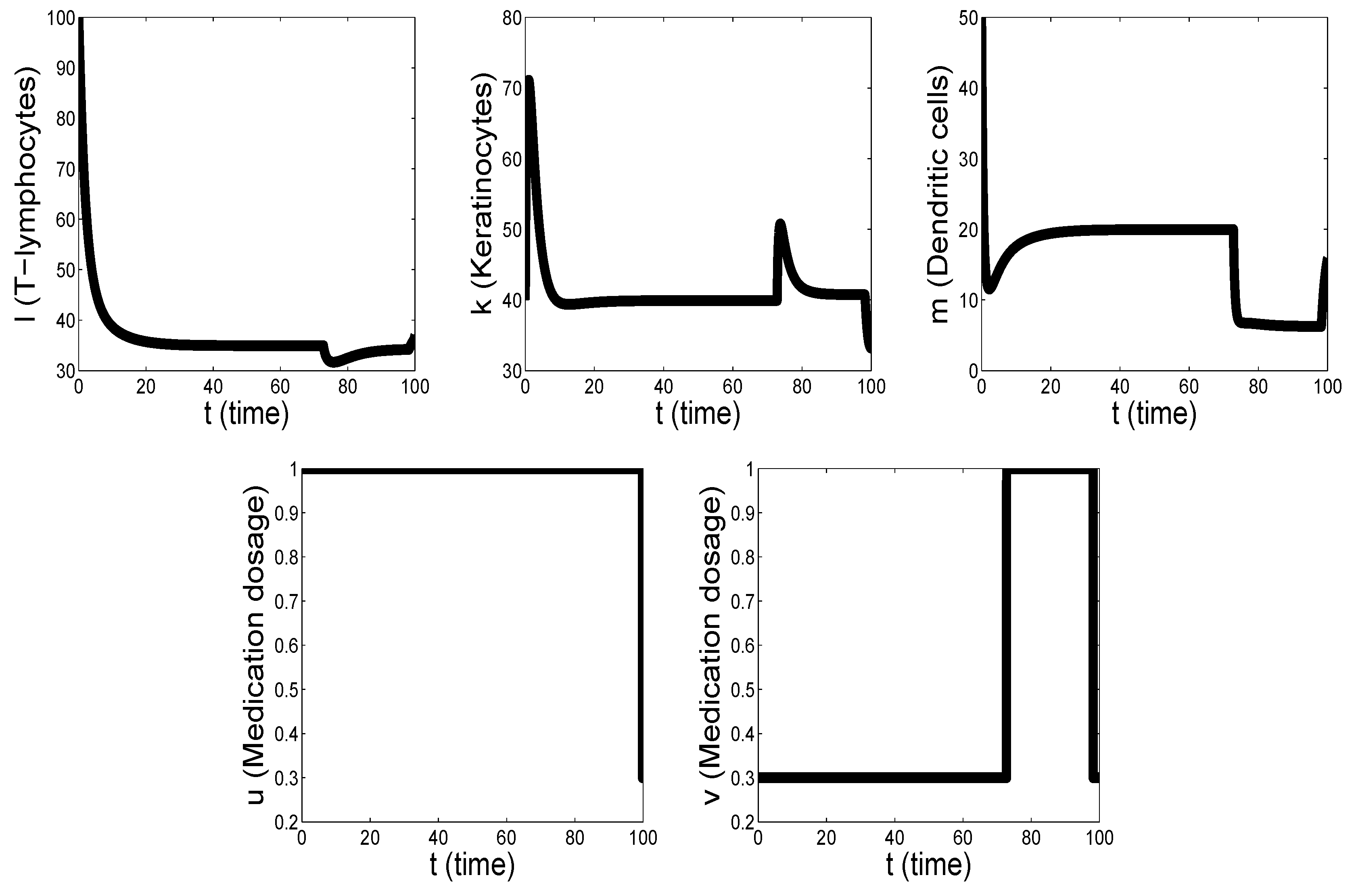
With the increase of the value of $\lambda$ (for example, $\lambda =1.2$), the actual optimal control ${\tilde{u}}_{*}(t)$ responsible for taking a drug that suppresses the interaction between T-lymphocytes and keratinocytes during most of the entire treatment period (95 days) has an interval corresponding to a smooth increase in the dosage of the used medication (singular arc). At the beginning and at the end of such an interval of psoriasis treatment there are the periods with increasing number of switchings from the lower intensity to the greatest intensity and vice versa (chattering). In addition, the whole process of this treatment ends with the interval of the greatest intensity (maximum dosage of the medication intake). Moreover, the schedule of taking a drug that suppresses the interaction between T-lymphocytes and dendritic cells does not qualitatively change. Almost during the entire period of psoriasis treatment (98 days), it is taken at the minimum dosage. Then, on the 99th day of the treatment period, the schedule for taking such a drug changes to the opposite. During the remaining two days it is taken at the maximum dosage.

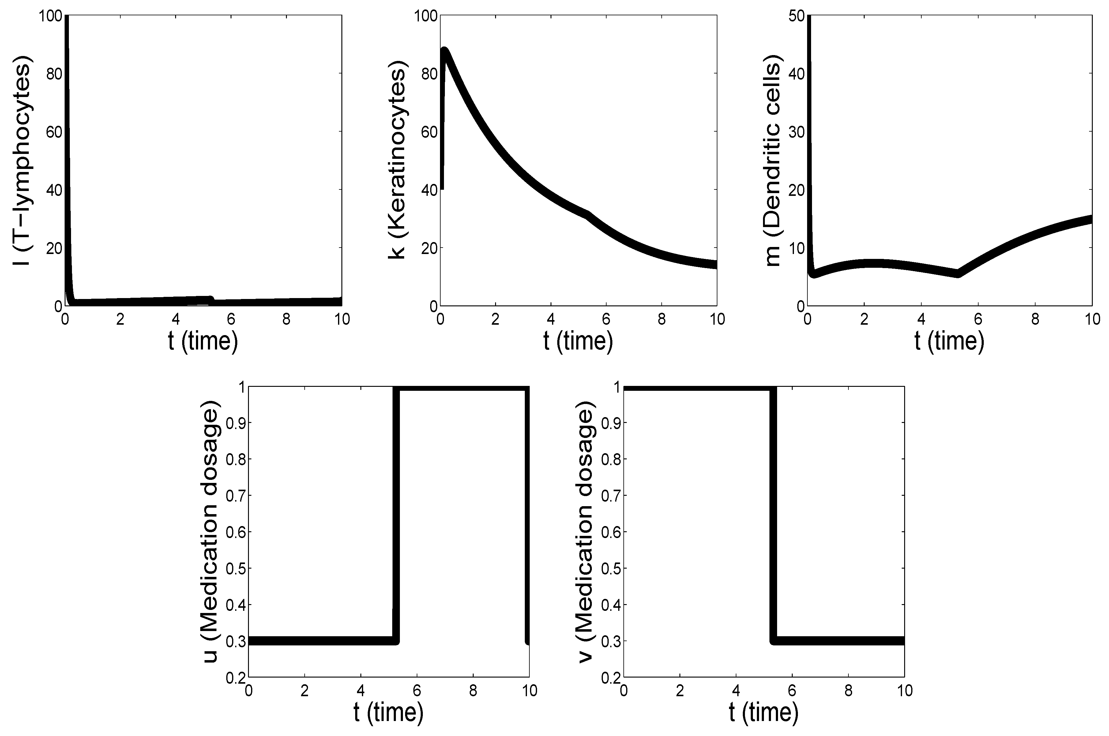
Next, it was found that with the decrease or increase of the length of psoriasis treatment (for example, 10 days or 190 days), the above schedule of the drugs intake does not qualitatively change. It should be noted only that with the reduction in the duration of this period, the first change in the schedule of taking medications begins to occur earlier (see Figure 3 and Figure 4 for 10 days), and with an increase in the duration of such a period, on the contrary, later (for example, 190 days).

Figure 3. Optimal solutions and optimal controls for $\lambda =0.3$: (upper row) $l_{*}(t)$, $k_{*}(t)$, $m_{*}(t)$; (lower row) $u_{*}(t)$, $v_{*}(t)$; $J_{*}=14.09275$.

Figure 4. Optimal solutions and optimal controls for $\lambda =1.2$: (upper row) $l_{*}(t)$, $k_{*}(t)$, $m_{*}(t)$; (lower row) $u_{*}(t)$, $v_{*}(t)$; $J_{*}=2.644754$.

From the comparison of the schedule of the medication intake for 100 days psoriasis treatment, one can conclude that a drug that suppresses the interaction between T-lymphocytes and keratinocytes predominates over a drug that suppresses the interaction between T-lymphocytes and dendritic cells. To show that this predominance is not absolute in psoriasis treatment, we (along with the values of the parameters of System (1), the initial values (2) and the control constraints (3) presented in (104), use the following values taken from [13]:

$$\begin{array}{cccc}\sigma =9.0\hfill & \rho =14.0\hfill & \beta =0.065\hfill & \delta =0.01\hfill \\ \lambda =0.4\hfill & \mu =0.07\hfill & \nu =0.02\hfill & T=100.0\hfill \\ {\gamma }_1=0.0032\hfill & {\gamma }_2=0.0002\hfill & u_{min}=0.3\hfill & v_{min}=0.3\hfill \\ l_0=100.0\hfill & k_0=40.0\hfill & m_0=50.0\hfill \end{array}$$

The corresponding results of the numerical calculations are given in Figure 5, which include the graphs of the optimal controls $u_{*}(t)$, $v_{*}(t)$, the corresponding optimal solutions $l_{*}(t)$, $k_{*}(t)$, and $m_{*}(t)$, and the minimum value of the functional $J(u,v)$ of (5). From the analysis of the graphs of controls $u_{*}(t)$, $v_{*}(t)$ and Formula (105), we conclude that for the majority of 100 days psoriasis treatment we use the maximum dosage of a drug suppressing the interaction between T-lymphocytes and dendritic cells. A drug that suppresses the interaction between T-lymphocytes and keratinocytes, should be used at the minimum dosage for 99 days and only on the last day the schedule of taking this medication should be changed to the maximum dosage. This is the first conclusion we draw from Figure 5. The second conclusion is that unlike the results shown in Figure 1 and Figure 3, the first change in the schedule of taking drugs does not occur simultaneously in both, but only in one, which suppresses the interaction between T-lymphocytes and dendritic cells.

Figure 5. Optimal solutions and optimal controls for $T=100.0$: (upper row) $l_{*}(t)$, $k_{*}(t)$, $m_{*}(t)$; (lower row) $u_{*}(t)$, $v_{*}(t)$; $J_{*}=33.185501$.

Figure 6 shows that with increasing duration of the period of psoriasis treatment (for example, to 150 days), the actual optimal control ${\tilde{v}}_{*}(t)$ responsible for taking a drug that suppresses the interaction between T-lymphocytes and dendritic cells has a period with a smooth increase in the dosage of the used medication (singular arc).

Figure 6. Optimal solutions and optimal controls for $T=150.0$: (upper row) $l_{*}(t)$, $k_{*}(t)$, $m_{*}(t)$; (lower row) $u_{*}(t)$, $v_{*}(t)$; $J_{*}=33.185511$.

Finally, the graphs of the optimal solution $k_{*}(t)$ from Figure 1, Figure 2, Figure 3, Figure 4, Figure 5 and Figure 6 show that the optimal concentration of keratinocytes $k_{*}(t)$ reaches at the end T of the interval $[0,T]$ the level, which is the minimal for the entire period $[0,T]$ of psoriasis treatment. This fact is very important for the treatment of the disease.

8. Conclusions

On a given time interval, a nonlinear system of three differential equations describing psoriasis treatment was considered. It established the relationships between the concentrations of T-lymphocytes, keratinocytes, and dendritic cells, which were its phase variables. Also, two scalar bounded controls were introduced into the system that reflected the doses of drugs aimed at suppressing interactions between T-lymphocytes and keratinocytes, as well as between T-lymphocytes and dendritic cells. The problem of minimizing the concentration of keratinocytes at the final moment of the time interval was stated for such a system. To analyze the optimal solution of the minimization problem consisting of the optimal controls and the corresponding optimal solutions of the original system, the Pontryagin maximum principle was applied. It allowed to obtain the Cauchy problem for the switching functions describing the behavior of the optimal controls. An analysis of this Cauchy problem showed that such controls could be either bang-bang functions, or, in addition to bang-bang intervals, they could contain singular arcs. Next, the possibility of simultaneous existence of singular arcs of the optimal controls was studied. The orders of singular arcs of such controls were found, the corresponding necessary optimality conditions for them were checked. Also, the forms of concatenations of singular arcs with nonsingular intervals (where the optimal controls are bang-bang functions) were investigated. After that, the finding of specific optimal solution to the considered minimization problem was carried out numerically using “BOCOP–2.0.5”. The corresponding results of calculations and their discussion were provided.