A New Approximation Method with High Order Accuracy

Abstract

In this paper, we propose a new multilevel univariate approximation method with high order accuracy using radial basis function interpolation and cubic B-spline quasi-interpolation. The proposed approach includes two schemes, which are based on radial basis function interpolation with less center points, and cubic B-spline quasi-interpolation operator. Error analysis shows that our method produces higher accuracy compared with other approaches. Numerical examples demonstrate that the proposed scheme is effective.

1. Introduction

The radial basis function (RBF) method is applied in a number of fields, such as multivariate function approximation, neural networks, and the solution of differential equations. It provides excellent interpolants for high dimensional scattered data sets, and its corresponding theory had been extensively studied by many researchers (see [1,2,3,4,5,6,7]). Unfortunately, we have to solve a linear system of equations by using RBF interpolation, and the system matrix becomes badly conditioned when the interpolating centers distributed densely. This was interpreted by the trade-off principle that is sometimes called the uncertainty relation proposed by Schaback [4]. To avoid this problem, many quasi-interpolation methods can be used in another way. In [8], the authors constructed two high accuracy multiquadric quasi-interpolation operators named ${\mathcal{L}}_{\mathcal{W}}$ and ${\mathcal{L}}_{{\mathcal{W}}_2}$ by using multi-level method via inverse multiquadric radial basis function (IMQ-RBF) interpolation, and Wu and Schaback’s MQ quasi-interpolation operator ${\mathcal{L}}_{\mathcal{D}}$. Moreover, in [9], ${\mathcal{L}}_{\mathcal{D}}$ was utilized to solve a one-dimensional Sine–Gordon equation with good numerical accuracy. Since the quasi-interpolation operator ${\mathcal{L}}_{\mathcal{D}}$ only have an $O\left(h^2\right)$ error if at least $c^2\left|\log c\right|=O\left(h^2\right)$, in this paper, B-spine quasi-interpolation with high order accuracy is considered. As the piecewise polynomial, spline—especially B-spline—have become a fundamental tool without solving any linear equations. Spline solutions of differential equations are implemented in many studies. B-splines of various degrees in the collocation and Galerkin methods were introduced for the numerical solutions of partial differential equations (PDEs) such as Burgers’ equation in [10,11,12,13,14,15,16]. Zhu and Wang [17] applied the cubic B-spline quasi-interpolation as a spatial approximation scheme, and a low order explicit finite difference method as a temporal approximation scheme to solve Burgers’ equation, and found that the numerical results are in good agreement with exact solutions.

In this paper, we construct a new multilevel scheme by using radial power RBF interpolation and cubic B-spline quasi-interpolation proposed by Sablonnière in [18]. The rest of this paper is organized as follows. In Section 2, some basic facts on RBF interpolation are introduced. In Section 3, we review some basic properties of cubic B-spline quasi-interpolation operator. The construction and the error estimate of the new quasi-interpolation method are studied in Section 4. Finally, some numerical examples are given in Section 5.

2. RBF Interpolation

RBF was introduced by Krige [19] in 1951 to deal with geological problems. Hitherto, RBFs were widely used in many fields (e.g., [1,5]). The process of interpolation by using RBF is as follows.

For a given region $\mathrm{\Omega }\in {\mathbb{R}}^d$ and a finite set $X=\{x_1,\cdots ,x_N\}\subset \mathrm{\Omega }$ of distinct points, we can construct an interpolant to a given function f of the form

$$S_{f,X}\left(x\right)=\sum _{i=1}^N{\alpha }_i\varphi (\parallel x-x_i{\parallel }_2)+\sum _{j=1}^Q{\beta }_j{p}_j\left(x\right),\mathrm{for}x\in \mathrm{\Omega },$$

(1)

where ${\parallel ·\parallel }_2$ denote the Euclidean norm, $\varphi :{\mathbb{R}}_{\ge 0}\to \mathbb{R}$ is a given RBF, and ${\left(p_j\right)}_{1\le j\le Q}$ is a basis of the space ${\mathbb{P}}_m^d$ of polynomials of degree at most m. The coefficients ${\alpha }_i$ and ${\beta }_j$ in the expressing (1) defining $S_{\varphi ,X}$ are determined by solving the linear system

$$\left\{\begin{array}{c}{\displaystyle \sum _{i=1}^N{\alpha }_i\varphi (\parallel x_k-x_i{\parallel }_2)+\sum _{j=1}^Q{\beta }_j{p}_j\left(x_k\right)=f\left(x_k\right),1\le k\le N,}\hfill \\ {\displaystyle \sum _{i=1}^N{\alpha }_i{p}_j\left(x_i\right)=0,1\le j\le Q.}\hfill \end{array}\right.$$

(2)

In this paper, we use α, β, and ${f|}_X$ instead of ${({\alpha }_1,\cdots ,{\alpha }_N)}^T$, ${({\beta }_1,\cdots ,{\beta }_Q)}^T$, and ${(f\left(x_1\right),\cdots ,f\left(x_N\right))}^T$, respectively. Solvability of this system is therefore equivalent to the solvability of the system

$$\left(\begin{array}{cc}{A}_{\varphi ,X}& P\\ P^T& 0\end{array}\right)\left(\begin{array}{c}\alpha \\ \beta \end{array}\right)=\left(\begin{array}{c}{f|}_X\\ 0\end{array}\right),$$

where $A_{\varphi ,X}=(\varphi (\parallel x_j-x_k{\parallel }_2))\in {\mathbb{R}}^{N\times N}$ and $P=\left(p_k\left(x_j\right)\right)\in {\mathbb{R}}^{N\times Q}$. System (2) is obviously solvable if the left-hand side (which is denoted by ${\tilde{A}}_{\varphi ,X}$) is invertible. From [2,3,20], we know that ${\tilde{A}}_{\varphi ,X}$ is invertible if $\varphi \left(r\right)$ is a conditional positive definite RBF of order m. If $m=0$, $\varphi \left(r\right)$ is said to be a strictly positive definite RBF. The most useful conditional positive definite RBFs of order m on ${\mathbb{R}}^d$ are given in Table 1, where the notation $\lceil t\rceil$ represents the smallest integer greater than or equal to $t\in \mathbb{R}$.

Table 1. The most useful conditional positive definite radial basis functions (RBFs). IMQ-RBF: inverse multiquadric RBF.

	$\mathit{\varphi }\left(\mathit{r}\right),\mathit{r}={\parallel \mathit{x}\parallel }_2,\mathit{c}>0$
Gaussians	$e^{-c{r}^2},$
Multiquadric RBFs	${(-1)}^{\lceil \mu /2\rceil }{(c^2+r^2)}^{\mu },\mu >0,\mu \notin {\mathbb{N}}_0$
Inverse Multiquadric RBFs	${(c^2+r^2)}^{\mu },\mu <0$
Thin-plate splines	${(-1)}^{k+1}{r}^{2k}\log \left(r\right),k\in \mathbb{N}$
Powers	${(-1)}^{\lceil k/2\rceil }{r}^k,k>0,k\notin 2{\mathbb{N}}_0$
Compactly Supported RBFs [6,21]	${\varphi }_{d,k}\left(r\right)$

The error estimate of the interpolation process using RBFs is considered taken place in the native space ${\mathcal{N}}_{\varphi }\left(\mathrm{\Omega }\right)$ determined by RBF ϕ and the region Ω. For strictly positive definite RBF ϕ, these spaces can be defined as the completion of the pre-Hilbert space

$$F_{\varphi }\left(\mathrm{\Omega }\right):={\mathrm{span}\left\{\varphi \right(\parallel ·-y\parallel }_2\left)\right|y\in \mathrm{\Omega }\},$$

equipped with the inner product

$${\left(\sum _{i=1}^M{a}_i\varphi (\parallel ·-x_i\parallel ),\sum _{j=1}^N{b}_j\varphi (\parallel ·-x_j\parallel )\right)}_{\varphi }:=\sum _{i=1}^M\sum _{j=1}^N{a}_i{b}_j\varphi (\parallel x_i-x_j\parallel ).$$

(3)

Since the error estimates are expressed in terms of the fill distance

$$h_{X,\mathrm{\Omega }}=\underset{x\in \mathrm{\Omega }}{\sup }\underset{x_j\in X}{\min }{\parallel x-x_j\parallel }_2,$$

therefore, the accuracy of approximation from $S_{f,X}$ to $f\in {\mathcal{N}}_{\varphi }\left(\mathrm{\Omega }\right)$ is studied for $h_{X,\mathrm{\Omega }}\to 0$. In this paper, we use a certain radial power RBF interpolation, so a theorem about error estimates of approximation by using IMQ-RBFs is given (see Section 11 in [5]).

Theorem 1.

Suppose that $\mathrm{\Omega }\subseteq {\mathbb{R}}^d$ is bounded and satisfies an interior cone condition. Let $\mathrm{\Phi }\left(x\right)={(-1)}^{\lceil k\rceil }{\parallel x\parallel }_2^k$, $k>0$, $k\notin 2{\mathbb{N}}_0$ be a power RBF. Denote the interpolant of a function $f\in {\mathcal{N}}_{\varphi }\left(\mathrm{\Omega }\right)$ based on this basis function and the set of centers $X=\{x_1,\cdots ,x_N\}\subseteq \mathrm{\Omega }$ by $S_{f,X}$. Then, there exists a constant $C>0$ such that the error between a function $f\in {\mathcal{N}}_{\varphi }\left(\mathrm{\Omega }\right)$ and its interpolant $S_{f,X}$ can be bounded by

$$\parallel f\left(x\right)-S_{f,X}{\left(x\right)\parallel }_{L_{\infty }\left(\mathrm{\Omega }\right)}\le C{h}_{X,\mathrm{\Omega }}^{k/2}·{\parallel f\parallel }_{{\mathcal{N}}_{\varphi }\left(\mathrm{\Omega }\right)},x\in \mathrm{\Omega },$$

with sufficiently small $h_{X,\mathrm{\Omega }}$.

3. Univariate B-Spline Quasi-Interpolants

For $I=[a,b]$, we denote by $S_d\left(X_n\right)$ the space of splines of degree d and $C^{d-1}$ on the uniform partition

$$X_n=\{x_i=a+ih,i=0,\cdots ,n\},$$

(4)

with meshlength $h=\frac{b-a}{n}$, where $b=x_n$. Let the B-spline basis of $S_d\left(X_n\right)$ be $\{B_j,j\in J\}$ with $J=\{1,2,\cdots ,n+d\}$, which can be computed by the de Boor–Cox formula [22]. Here, we add multiple knots at the endpoints: $a=x_{-d}=x_{-d+1}=\cdots =x_0$ and $b=x_n=x_{n+1}=\cdots =x_{n+d}$.

Univariate B-spline quasi-interpolants (QIs) can be defined as operators of the form

$$Q_{d}f=\sum _{j\in J}{\mu }_j{B}_j.$$

We denote by ${\prod }_d$ the space of polynomials of total degree at most d. In general, we impose that $Q_d$ is exact on the space ${\prod }_d$; i.e., $Q_d\left(p\right)=p$ for all $p\in {\prod }_d$, then the approximation order of $Q_d$ is $O\left(h^{d+1}\right)$ on smooth functions. In [18,23], the coefficient ${\mu }_j$ is a linear combination of discrete values of f at some point in the neighborhood of $supp\left(B_j\right)=[x_{j-d-1},x_j]$. The main advantage of QIs is that they have an explicit construction and there is no need to solve any system of linear equations. Since the cubic spline has become the most commonly used spline, in this paper, we use cubic B-spline quasi-interpolation.

Let $y_i=f\left(x_i\right),i=0,1,\cdots ,n,$ be the coefficients of the cubic B-spline quasi-interpolant

$$Q_{d}f=\sum _{j=1}^{n+3}{\mu }_j\left(f\right)B_j$$

(5)

are

$$\begin{array}{cc}\hfill {\mu }_1\left(f\right)& =y_0\hfill \\ \hfill {\mu }_2\left(f\right)& =\frac{1}{18}\left(7y_0+18y_1-9y_2+2y_3\right),\hfill \\ \hfill {\mu }_j\left(f\right)& =\frac{1}{6}\left(-y_{j-3}+8y_{j-2}-y_{j-1}\right),j=3,\cdots ,n+1,\hfill \\ \hfill {\mu }_{n+2}\left(f\right)& =\frac{1}{18}\left(2y_{n-3}-9y_{n-2}+18y_{n-1}+7y_n\right),\hfill \\ \hfill {\mu }_{n+3}\left(f\right)& =y_n.\hfill \end{array}$$

(6)

For $f\in C^4\left(I\right)$, we have the error estimate [18]

$$\parallel f-Q_d{f\parallel }_{\infty }\le C{\left|f^{\left(4\right)}\right|}_{\infty }·h^4,C\in \mathbb{R}.$$

(7)

4. New Quasi-Interpolation Method

From the above two sections, we note that we can get high approximation order by using RBFs interpolation, however, we have to solve an unstable linear system of equations when the number of interpolation centers increases. This drawback can be avoided by considering various methods; for instance, it is possible to use partition of unity methods [24,25] or Shepard’s like methods [26,27,28,29,30,31,32]. This problem can also be avoided by using B-spline quasi-interpolation. So, we construct a new quasi-interpolation operator $Q_r$ which possess the advantages of RBFs interpolation and B-spline quasi-interpolation.

For any function $f\in C^4$ and equispaced points (4). Let us fix $N<n$, and $0<k_1<k_2<\cdots <k_N<n$. Under these assumptions, let us suppose that the set of data ${\left\{\left(x_{k_j},f^{\left(4\right)}\left(x_{k_j}\right)\right)\right\}}_{j=1}^N$ is given, and that

$$X_N=\{x_{k_1},\cdots ,x_{k_N}\},h_2:=\underset{2\le i\le N}{\max }(x_{k_i}-x_{k_{i-1}}).$$

Then, according to Section 1, we can get an RBF interpolant $S_{f^{\left(4\right)},X_N}$ to approximate the fourth-order derivative of $f\left(x\right)$ on $[a,b]$, and satisfying

$$S_{f^{\left(4\right)},X_N}\left(x_{k_i}\right)=f^{\left(4\right)}\left(x_{k_i}\right),i=1,\cdots ,N.$$

Here, we use the power RBF

$$\varphi \left(r\right)=\parallel r\parallel ,$$

which can be derived from the fourth-order derivative of high power function

$$\psi \left(r\right)=\frac{1}{120}{\parallel r\parallel }^5.$$

Since $\varphi \left(r\right)$ is strictly positive definite function [7], we can express the interpolant $S_{f^{\left(4\right)},N}$ as follows:

$$S_{f^{\left(4\right)},X_N}\left(x\right)=\sum _{i=1}^N{\alpha }_i\varphi \left(\right|x-x_{k_i}\left|\right),$$

(8)

and the coefficients ${\left\{{\alpha }_i\right\}}_{i=1}^N$ are determined by the interpolation conditions

$$S_{f^{\left(4\right)},X_N}\left(x_{k_j}\right)=\sum _{i=1}^N{\alpha }_i\varphi \left(\right|x_{k_j}-x_{k_i}\left|\right)=f^{\left(4\right)}\left(x_{k_j}\right),j=1,\cdots ,N.$$

(9)

Let us denote by

$$\begin{array}{c}{\mathrm{\Psi }}_{X_N}=\left(\varphi \left(\right|x-x_{k_1}\left|\right),\cdots ,\varphi \left(\right|x-x_{k_N}|\right),\alpha ={({\alpha }_1,\cdots ,{\alpha }_N)}^T,\hfill \\ A_{\varphi ,X_N}=\left(\varphi \right(|x_{k_j}-x_{k_i}{\left|\right))}_{1\le i,j\le N},f_{X_N}^{\left(4\right)}={(f^{\left(4\right)}\left(x_{k_1}\right),\cdots ,f^{\left(4\right)}\left(x_{k_N}\right))}^T,\hfill \end{array}$$

(10)

from Section 1, we know that Equation (9) is solvable, so

$$\alpha ={\left(A_{\varphi ,X_N}\right)}^{-1}·f_{X_N}^{\left(4\right)}.$$

(11)

Moreover, $S_{f^{\left(4\right)},X_N}\left(x\right)$ defined in (8) has a Lagrange-type representation

$$S_{f^{\left(4\right)},X_N}\left(x\right)=\sum _{i=1}^N{u}_i\left(x\right)f^{\left(4\right)}\left(x_{k_i}\right).$$

(12)

Let us suppose that $U\left(x\right)=\left(u_1\left(x\right),\cdots ,u_N\left(x\right)\right)$; by Equations (8) and (12), we get

$$U\left(x\right)={\mathrm{\Psi }}_{X_N}·{\left(A_{\varphi ,X_N}\right)}^{-1}·f_{X_N}^{\left(4\right)}.$$

By using f and the coefficient α defined in (11), we construct a function in the form

$$e\left(x\right)=f\left(x\right)-\sum _{i=1}^N{\alpha }_i\psi \left(\right|x-x_{k_i}\left|\right).$$

(13)

Then, we can define a MQ quasi-interpolation by using $Q_d$ defined by (5) and (6) on the data ${\left(x_i,e\left(x_i\right)\right)}_{1\le i\le n}$, and then the new quasi-interpolation operator is presented as

$$Q_{r}f\left(x\right)=\sum _{i=1}^N{\alpha }_i\psi \left(\right|x-x_{k_i}\left|\right)+Q_{d}e\left(x\right).$$

(14)

According to the above section, we know that the quasi-interpolation $Q_r$ is composed of power interpolation and $Q_d$ quasi-interpolation. As we mentioned in Section 1, the error estimate for $\varphi \left(r\right)=\parallel r\parallel$ interpolation is considered in a native space ${\mathcal{N}}_{\varphi }$. Let f be such that $f^{\left(4\right)}\left(x\right)\in {\mathcal{N}}_{\varphi }$. According to (13), (14), and (7), we have

$$\begin{array}{cc}\hfill \parallel f-Q_{r}f{\parallel }_{\infty }& ={\parallel f-\sum _{i=1}^N{\alpha }_i\psi \left(\right|·-x_{k_i}\left|\right)-Q_{d}e\parallel }_{\infty }\hfill \\ & =\parallel e-Q_d{e\parallel }_{\infty }\le C{\parallel e^{\left(4\right)}\parallel }_{\infty }·h^4.\hfill \end{array}$$

(15)

Since

$$\begin{array}{cc}\hfill \parallel e^{\left(4\right)}{\parallel }_{\infty }& ={\parallel f^{\left(4\right)}-\sum _{i=1}^N{\alpha }_i{\psi }^{\left(4\right)}\left(\right|·-x_{k_i}\left|\right)\parallel }_{\infty }\hfill \\ & ={\parallel f^{\left(4\right)}-\sum _{i=1}^N{\alpha }_i\varphi \left(\right|·-x_{k_i}\left|\right)\parallel }_{\infty }={\parallel f^{\left(4\right)}-\sum _{i=1}^N{u}_i{f}^{\left(4\right)}\left(x_{k_i}\right)\parallel }_{\infty }.\hfill \end{array}$$

(16)

From (12), we can easily get that (16) is the error estimate of power interpolation to $f^{\left(4\right)}\left(x\right)$.

From Theorem 1 and (16), we can get

$$\parallel f-Q_r{f\parallel }_{\infty }\le C{\parallel f^{\left(4\right)}\parallel }_{{\mathcal{N}}_{\varphi }}·h_{X_N,I}^{k/2}·h^4,C\in {\mathbb{R}}^{+}.$$

(17)

So, we conclude our result on the error estimate of the quasi-interpolant $Q_r$ as follows:

Theorem 2.

For a given function f, suppose that $f^{\left(4\right)}\in {\mathcal{N}}_{\varphi }$. Then, there exists a constant $C>0$ such that

$$\parallel f-Q_r{f\parallel }_{\infty }\le C{\parallel f^{\left(4\right)}\parallel }_{{\mathcal{N}}_{\varphi }}·h_{X_N,I}^{k/2}·h^4.$$

5. Numerical Example

We consider the following function

$$f\left(x\right)=x^9,$$

given in [8], and use $Q_r$ to approximate it. Moreover, we compare the error with $Q_d$ and power interpolation; here we adopt $l_{\infty }$-norm that is taken to be the maximum absolute error at the $2^9$ equally spaced points on $[0,1]$.

The profile of the function is shown in Figure 1. For convenience, we set $h_2/4=h=0.025$, and $x_{k_i}=h_2^i$, $(i=0,\cdots ,N=4)$, then the approximation error using by $Q_r$ is shown in Figure 2, the approximation error using by $Q_d$ is shown in Figure 3, and the approximation error using by power interpolation with $h_2=0.1$ is shown in Figure 4. From these examples, we can see that the approximation effect of $Q_r$ is much better than $Q_d$ and power interpolation.

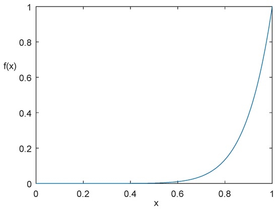
Figure 1. The graph of $f\left(x\right)$.

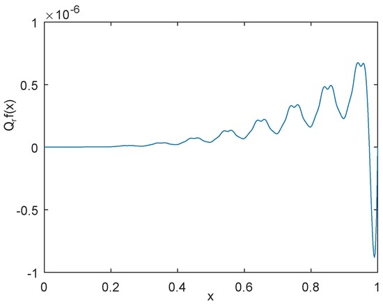
Figure 2. The graph of error using by $Q_r$ with $h_2/4=h=0.025$.

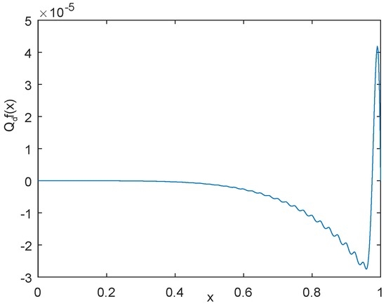
Figure 3. The graph of error using by $Q_d$ with $h=0.025$.

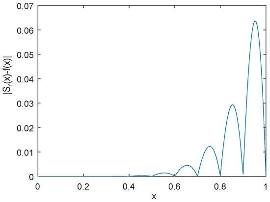
Figure 4. The graph of error using by power interpolation with $h_2=0.1$.

6. Conclusions

In this paper, we construct a new quasi-interpolation $Q_r$ based on power interpolation and $Q_d$ scheme. Our scheme has the advantages of higher approximation order. Besides that, it can avoid ill-condition problems compared with RBFs interpolation. From the numerical example, we can see that the accuracy is much better than $Q_d$ and power interpolation themselves. However, it would be interesting to compare the proposed method with other methods present in literature as a future work, as for example the operators proposed in [26,33], using appropriate test functions.

References

- Buhmann, M.D. Radial Basis Functions. Theory and Implementations; Cambridge University Press: Cambridge, UK, 2003. [Google Scholar]
- Micchelli, C.A. Interpolation of scattered data: Distance matrices and conditionally positive definite functions. Constr. Approx. 1986, 2, 11–22. [Google Scholar] [CrossRef]
- Powell, M.J.D. The theory of radial basis function approximation in 1990. In Advances in Numerical Analysis; Light, W., Ed.; Oxford Scinece Publications: Oxford, UK, 1992; Volume II. [Google Scholar]
- Schaback, R. Error estimates and condition number for radial basis function interpolation. Adv. Comput. Math. 1995, 3, 251–264. [Google Scholar] [CrossRef]
- Wendland, H. Scattered data approximation. In Cambridge Monographs on Applied and Computational Mathematics; Cambridge University Press: Cambridge, UK, 2005; Volume 17. [Google Scholar]
- Wu, Z.M. Compactly supported positive definite radial functions. Adv. Comput. Math. 1995, 4, 283–292. [Google Scholar] [CrossRef]
- Fasshauer, G.E. Meshfree Approximation Methods with Matlab; World Scientific Publishing: Singapore, 2007. [Google Scholar]
- Jiang, Z.W.; Wang, R.H.; Zhu, C.G.; Xu, M. High Accuracy Multiquadric Quasi-interpolation. Appl. Math. Model. 2011, 35, 2185–2195. [Google Scholar] [CrossRef]
- Jiang, Z.W.; Wang, R.H. Numerical solution of one-dimensional SineCGordon equa- tion using high accuracy multiquadric quasi-interpolation. Appl. Math. Comput. 2012, 218, 7711–7716. [Google Scholar]
- Ali, H.A.; Gardner, R.T.; Gardner, G.A. A collocation method for Burgers’ equation using cubic B-splines. Comput. Methods Appl. Mech. Eng. 1992, 100, 325–337. [Google Scholar] [CrossRef]
- Dağ, İ.; Irk, D.; Saka, B. A numerical solution of the Burgers’ equation using cubic B-splines. Appl. Math. Comput. 2005, 163, 199–211. [Google Scholar] [CrossRef]
- Dağ, İ.; Saka, B.; Boz, A. B-spline Galerkin methods for numerical solutions of the Burgers’ equation. Appl. Math. Comput. 2005, 166, 506–522. [Google Scholar] [CrossRef]
- Ramadan, M.A.; El-Danaf, T.S.; Alaal, F. A numerical solution of the Burgers’ equation using septic B-splines. Chaos Solitons Fract. 2005, 26, 795–804. [Google Scholar] [CrossRef]
- Saka, B.; Dağ, İ. Quartic B-spline collocation methods to the numerical solutions of the Burgers’ equation. Chaos Solitons Fract. 2007, 32, 1125–1137. [Google Scholar] [CrossRef]
- Saka, B.; Dağ, İ. A numerical study of the Burgers’ equation. J. Frankl. Inst. 2008, 345, 328–348. [Google Scholar] [CrossRef]
- Zaki, S.I. A quintic B-spline finite elements scheme for the KdVB equation. Comput. Methods Appl. Eng. 2000, 188, 121–134. [Google Scholar] [CrossRef]
- Zhu, C.G.; Wang, R.H. Numerical solution of Burgers’ equation by cubic B-spline quasi-interpolation. Appl. Math. Comput. 2009, 208, 260–272. [Google Scholar] [CrossRef]
- Sablonnière, P. Univariate spline quasi-interpolants and applications to numerical analysis. Rend. Sem. Mat. Univ. Pol. Torino 2005, 63, 211–222. [Google Scholar]
- Krige, D.G. A Statistical Approach to Some Mine Valuation and Allied Problems on the Witwatersrand. Master’s Thesis, University of Witwatersrand, Johannesburg, South Africa, 1951. [Google Scholar]
- Madych, W.R. Miscellaneous error bounds for multiquadric and related interpolators. Comput. Math. Appl. 1992, 24, 121–138. [Google Scholar] [CrossRef]
- Wendland, H. Piecewise polynomial, positive definite and compactly supported radial functions of minimal degree. Adv. Comput. Math. 1995, 4, 389–396. [Google Scholar] [CrossRef]
- De Boor, C. A Practical Guide to Splines; Revised edition; Springer: New York, NY, USA, 2001. [Google Scholar]
- Sablonnière, P. Quasi-interpolants splines sobre particiones uniforms. In Proceedings of the 1st Meeting in Approximation Theory of the University of Jaén, Ubeda, Spain, 29 June–2 July 2000; Prépublication IRMAR 00-38. Rennes, France, June 2000. [Google Scholar]
- Cavoretto, R.; De Marchi, S.; De Rossi, A.; Perracchione, E.; Santin, G. Partition of unity interpolation using stable kernel-based techniques. Appl. Numer. Math. 2016. [Google Scholar] [CrossRef]
- Cavoretto, R.; De Rossi, A.; Perracchione, E. Efficient computation of partition of unity interpolants through a block-based searching technique. Comput. Math. Appl. 2016, 71, 2568–2584. [Google Scholar] [CrossRef]
- Caira, R.; Dell’Accio, F. Shepard-Bernoulli operators. Math Comput. 2007, 76, 299–321. [Google Scholar] [CrossRef]
- Caira, R.; Dell’Accio, F.; Di Tommaso, F. On the bivariate Shepard-Lidstone operators. J. Comput. Appl. Math. 2012, 236, 1691–1707. [Google Scholar] [CrossRef]
- Dell’Accio, F.; Di Tommaso, F. Scattered data interpolation by Shepard’s like methods: Classical results and recent advances, Dolomites Research Notes on Approximation. Dolomites Res. Notes Approx. 2016, 9, 32–44. [Google Scholar]
- Costabile, F.A.; Dell’Accio, F.; Di Tommaso, F. Enhancing the approximation order of local Shepard operators by Hermite polynomials. Comput. Appl. Math. 2012, 64, 3641–3655. [Google Scholar] [CrossRef]
- Costabile, F.A.; Dell’Accio, F.; Di Tommaso, F. Complementary Lidstone interpolation on scattered data sets. Numer. Algorithms 2013, 64, 157–180. [Google Scholar] [CrossRef]
- Dell’Accio, F.; Di Tommaso, F. Complete Hermite-Birkhoff interpolation on scattered data by combined Shepard operators. J. Comput. Appl. Math. 2016, 300, 192–206. [Google Scholar] [CrossRef]
- Dell’Accio, F.; Di Tommaso, F.; Hormann, K. On the approximation order of triangular Shepard interpolation. IMA J. Numer. Anal. 2016, 36, 359–379. [Google Scholar] [CrossRef]
- De Marchi, S.; Dell’Accio, F.; Mazza, M. On the constrained mock-Chebyshev least-square. J. Comput. Appl. Math. 2015, 280, 94–109. [Google Scholar] [CrossRef]
© 2017 by the author; licensee MDPI, Basel, Switzerland. This article is an open access article distributed under the terms and conditions of the Creative Commons Attribution (CC-BY) license (http://creativecommons.org/licenses/by/4.0/).