Article

Rational Spline Image Upscaling with Constraint Parameters

1
School of Computer Science and Technology, Shandong University of Finance and Economics, Jinan 250014, China
2
School of Mathematics, Shandong University, Jinan 250100, China
3
School of Computer Science and Technology, Shandong University, Jinan 250101, China
*
Author to whom correspondence should be addressed.
Math. Comput. Appl. 2016, 21(4), 48; https://doi.org/10.3390/mca21040048
Submission received: 30 September 2016 / Revised: 14 November 2016 / Accepted: 14 November 2016 / Published: 13 December 2016
(This article belongs to the Special Issue Information and Computational Science)

Abstract

:
Image interpolation is one of key contents in image processing. We present an interpolation algorithm based on a rational function model with constraint parameters. Firstly, based on the construction principle of the rational function, the detection threshold is selected through contour analysis. The smooth and non-smooth areas are interpolated by bicubic interpolation and general rational interpolation, respectively. In order to enhance the contrast in non-smooth areas and preserve the details, the parameter optimization technique is applied to get optimal shape parameters. Experimental results on benchmark test images demonstrate that the proposed method achieves competitive performance with the state-of-the-art interpolation algorithms, especially in image details and texture features.

1. Introduction

Interpolation acts as a bridge between the continuous world and the discrete one. As an important technique, it pervades many applications [1,2]. A digital image is not an exact snapshot of reality, it is only a discrete approximation. Image interpolation focuses on the issue which obtains a high-resolution image from a low-resolution one. Image interpolation plays an important role in image processing, and it is widely used in various fields, such as aerospace, medical, military, scientific research, communications, remote sensing satellite, television, film production, etc.
Generally speaking, the interpolation technique is used in nearly every geometric transformation, such as translation, scaling, rotation, etc. Such operations are utilized in many commercial digital image processing software [3]. The main issue of image interpolation is to maintain texture details and edge structure, while eliminating blocking artifacts, texture disorder, and other visual artifacts. Quantities of image interpolation methods have been proposed in several articles [4,5,6,7,8,9,10,11,12,13]. In these existing methods, linear filters (as the simplest technique) have been widely used in image interpolation, such as the bilinear, bicubic [4], and cubic spline algorithms [5]. Although these traditional methods are effective, they have disadvantages in ringing artifacts, blurred details, and so forth. Because the image can be affected by many factors, including the light, natural background, and the characteristics of its own texture, all in all, the relationship between pixels is not linear [14].
With ever-increasing capacity of computation power, many image interpolation methods have been proposed in the past few years. Jeong et al. [15] presented a multi-frame example-based super-resolution (SR) algorithm using locally directional self-similarity. Jha et al. [16] proposed a new image interpolation method using adaptive weights based on inverse gradients and distances from the pixels used in prediction. In [17], an edge-guided interpolation approach was proposed, which improved the accuracy of interpolation by detecting edges and fitting them with templates. In [18], predetermined edge patterns were used to obtain optimal parameters. As a consequence, according to the original images’ edge structures, high quality interpolated images could be obtained. Edge-Directed interpolation (EDI) methods have been presented [19]. Said and Pearlman [20] proposed a source model which focuses on the integrity of detected edges and modifies the interpolation to adapt to the original one. Then, a New Edge-Directed Interpolation (NEDI) adaptive method was presented, which obtains better subjective quality than EDI. Based on the geometric duality between the low-resolution covariance and the high-resolution covariance, the relationship of high-resolution covariance and the low-resolution one can be estimated [6]. A soft-decision interpolation technique (SAI) was proposed, which estimates unknown pixels in groups [13].
We dedicated our research to the integration of image interpolation and human visual perception. However, how to design the interpolation algorithm that combines with visual perception for the purpose of getting an “ideal” interpolated image is still a challenge for image interpolation methods. In this paper, a new image interpolation method based on rational function model is proposed. Considering the speed and quality of the interpolated image, the input image will be classified into smooth areas and non-smooth areas. For smooth areas, a bicubic interpolation is used to lower time complexity. For non-smooth areas, the proposed optimal rational interpolation function is used to improve the accuracy of interpolation. The bicubic interpolation function is a special form of the same interpolation function model on the condition that the parameters are chosen with some specific values. Namely, parameters α and β equal 1. The mean value of nine interpolation data points is the threshold, and is used for non-smooth area detection. Image interpolation, processing, region detection, different region interpolation, and visual contrast enhancement are all based on one rational interpolation model. Experimental results show good image quality results in both edges and details. The algorithm framework is shown in Figure 1.
This paper is organized as follows: Section 2 introduces the fundamental principles of the rational function model and its properties. Section 3 presents the proposed interpolation algorithm. Experimental results are shown for demonstration in Section 4. Section 5 concludes this paper.

2. A Bivariate Rational Interpolation

In recent years, the univariate rational spline interpolations with parameters have been developed [21,22,23]. These kinds of interpolation splines have a simple mathematical representation and can preserve property of interpolated curve and surface. Motivated by the univariate rational spline interpolation, the bivariate rational interpolation with parameters based on the function values has been studied in [24,25,26,27,28,29]. The interpolation function has a piecewise explicit rational mathematical representation with parameters, and it can be represented by its basis.
Let Ω : [ a , b ; c , d ] be the plane region, let f ( x , y ) be a bivariate function defined in the region Ω, and let a = x 1 < x 2 < < x n < x n + 1 = b and c = y 1 < y 2 < < y m < y m + 1 = d be the knot sequences. Denote f ( x i , y j ) by f i , j ; then, { ( x i , y j , f i , j ) , i = 1 , 2 , n , n + 1 ; j = 1 , 2 , m , m + 1 } are the given set of data points. For any point ( x , y ) [ x i , x i + 1 ; y j , y j + 1 ] in the x y -plane, let h i = x i + 1 x i , θ = x x i h i , and l j = y j + 1 y j , η = y y j l j . For each y = y j , j = 1 , 2 , m + 1 , construct the x-direction interpolation curve; this is given by
P i , j * ( x ) = p i , j * ( x ) q i , j * ( x ) , x [ x i , x i + 1 ] , i = 1 , 2 , n 1 ,
where
p i , j * ( x ) = ( 1 θ ) 3 α i , j f i , j + θ ( 1 θ ) 2 V i , j * + θ 2 ( 1 θ ) W i , j * + θ 3 f i + 1 , j , q i , j * ( x ) = ( 1 θ ) α i , j + θ ,
and
V i , j * = ( α i , j + 1 ) f i , j + α i , j f i + 1 , j , W i , j * = ( α i , j + 2 ) f i + 1 , j h i Δ i + 1 , j * ,
with α i , j > 0 , and Δ i , j * = ( f i + 1 , j f i , j ) / h i . This interpolation is called the rational cubic interpolation based on function values which satisfies
p i , j * ( x i ) = f i , j , p i , j * ( x i + 1 ) = f i + 1 , j ,
p i , j * ( x i ) = Δ i , j * , p i , j * ( x i + 1 ) = Δ i + 1 , j * .
Obviously, the interpolation is a local one, it is defined in the interval [ x i , x i + 1 ] and depends on the data at three points { ( x r , y j , f r , j ) , r = i , i + 1 , i + 2 } and the parameter α i , j .
For each pair ( i , j ) , i = 1 , 2 , n 1 and j = 1 , 2 , m 1 , using the x-direction interpolation function P i , j * ( x ) , define the bivariate rational interpolating function P i , j ( x , y ) on [ x i , x i + 1 ; y j , y j + 1 ] as follows
P i , j ( x , y ) = p i , j ( x , y ) q i , j ( y ) , i = 1 , 2 , , n 1 ; j = 1 , 2 , , m 1
where
p i , j ( x , y ) = ( 1 η ) 3 β i , j P i , j * ( x ) + η ( 1 η ) 2 V i , j + η 2 ( 1 η ) W i , j + η 3 P i , j + 1 * ( x ) , q i , j ( y ) = ( 1 η ) β i , j + η ,
and
V i , j = ( β i , j + 1 ) P i , j * ( x ) + β i , j P i , j + 1 * ( x ) , W i , j = ( β i , j + 2 ) P i , j + 1 * ( x ) l j Δ i , j + 1 ( x ) ,
with β i , j > 0 , and Δ i , j ( x ) = ( P i , j + 1 * ( x ) P i , j * ( x ) ) / l j .
In the subregion [ x i , x i + 1 ; y j , y j + 1 ] , the function P i , j ( x , y ) is called a bivariate rational interpolation function based on function values. It depends on the data at nine points { ( x r , y s , f r , s ) , r = i , i + 1 , i + 2 , s = j , j + 1 , j + 2 } and which satisfies
P i , j ( x r , y s ) = f ( x r , y s ) ,   r = i , i + 1 ,   s = j , j + 1 .
Consider the equally spaced knots case; namely, for all i = 1 , 2 , , n and j = 1 , 2 , , m , h i = h j and l i = l j . The interpolating function P i , j ( x , y ) is C 1 in the whole interpolating region. The bivariate rational interpolating function P i , j ( x , y ) can be expressed as follows:
P i , j ( x , y ) = r = 0 2 s = 0 2 ω r s ( θ , α i ; η , β j ) f i + r , j + s
where
ω r s ( θ , α i ; η , β j ) = ω r ( θ , α i ) ω s ( η , β j )
ω 0 ( θ , α i ) = ( 1 θ ) 2 ( α i + θ ) ( 1 θ ) α i + θ
ω 1 ( θ , α i ) = θ ( 1 θ ) α i + 3 θ 2 2 θ 3 ( 1 θ ) α i + θ
ω 2 ( θ , α i ) = θ 2 ( 1 θ ) ( 1 θ ) α i + θ .
The terms ω r s ( θ , α i ; η , β j ) ,   r = 0 , 1 , 2 ;   s = 0 , 1 , 2 are called the basis of the bivariate interpolation, which satisfy
r = 0 2 s = 0 2 ω r s ( θ , α i ; η , β j ) = 1 .
From Equation (3), the interpolating function P i , j ( x , y ) is defined by a given set of data points { f i , j ,   f i + 1 , j ,   f i + 2 , j ;   f i , j + 1 , f i + 1 , j + 1 ,   f i + 2 , j + 1 ;   f i , j + 2 ,   f i + 1 , j + 2 ,   f i + 2 , j + 2 } . Applying the interpolating function, we can construct a patch through points f i , j , f i + 1 , j ,   f i , j + 1 , f i + 1 , j + 1 .

3. Basic Algorithms

Generally speaking, there is always a contradiction between the processing speed of interpolation and the resultant quality in image interpolation. The commonly used methods [6,7,13] usually adopt different interpolation functions for different regions Furthermore, the different region detection algorithm is not related to the interpolation. Namely, the used methods are not based on the interpolation function. Because the image has natural attributes, its inherent attributes are inevitably affected by using the commonly used methods. Thus, we present a novel interpolation model to solve this problem. Moreover, the processing speed of interpolation and the resultant quality are all preserved using the new algorithm.

3.1. Image Non-Smooth Areas Detection

In this paper, a variety of textures and edges of the image area are called non-smooth areas. The smooth areas contain abundant detailed information, and have critical effects on the image quality. First of all, the non-smooth areas are detected.
From the rational function, a patch can be constructed given nine data points. All of them have different effects on the patch through their weights ω r s ( θ , α ; η , β ) . When the weights present great differences from each other, the patch becomes more and more non-flat, considered as non-smooth area in the interpolated image. As mentioned above, the data points play a different role in the structure processing. The drawing and analyses of contours depends on the decision of the sign. On this basis, contour analysis is used to detect the non-smooth areas. The detection model is based on the interpolation model. As mentioned above, an interpolated patch is constructed using nine data points. The points play different roles in the structure processing. The vertices of the patch are the key points. The other data points are auxiliary. As the detection threshold, the mean value of the nine data points can be used for detecting the non-smooth areas in the interpolated image. Namely, for any given set of data r = 0 2 s = 0 2 f r , s , r , s = 0 , 1 , 2 , the detection threshold λ is given as follows:
λ = r = 0 2 s = 0 2 f r , s 9 .
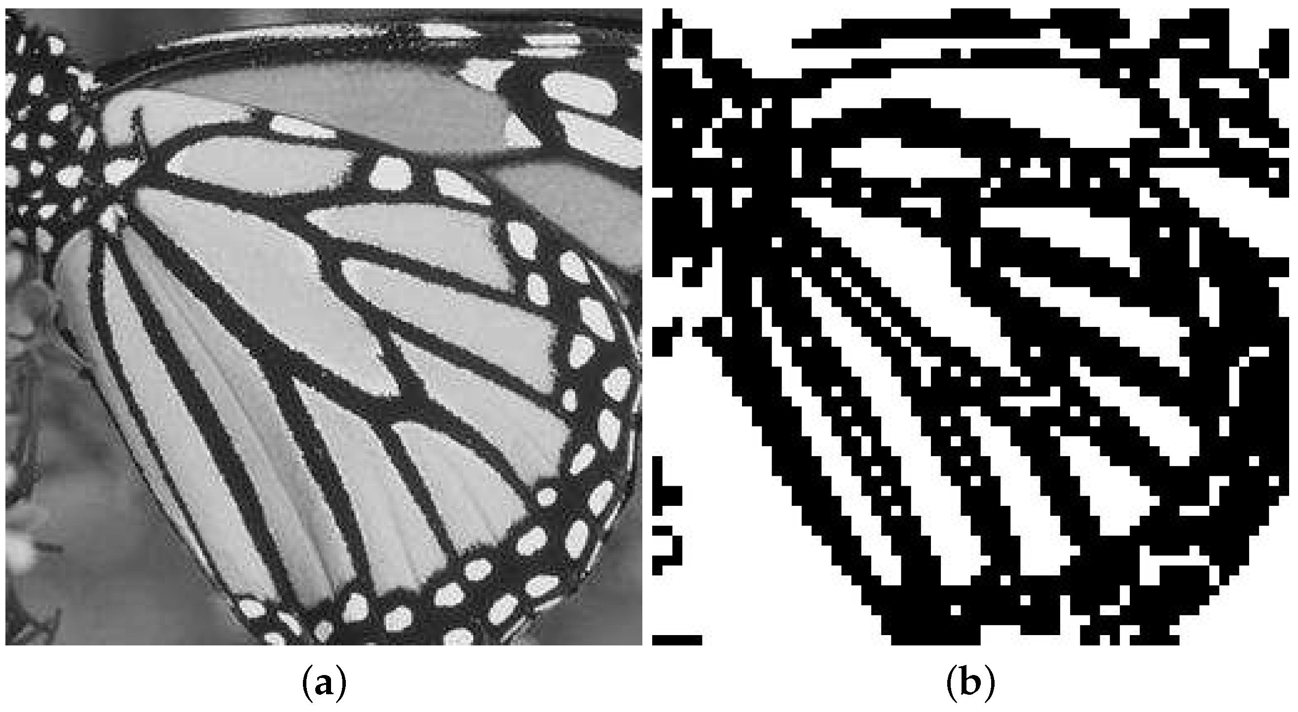
Let δ = f r , s λ , r , s = 0 , 1 ; from the contours drawing and analyses, if δ are all nonpositive and have nonnegative sign, the region is regarded as non-smooth. Otherwise it is smooth. Basically, the detection threshold is selected based on the rational function construction. The non-smooth detection results are shown in Figure 2.

3.2. Image Interpolation

An image is a set of values on a 2D plane. It is affected by the material of the object surface, the physical appearance of background objects , light strength and angle, and noise of the imaging progress. These data are purely random and can be constructed completely. The value of these data are gradually changed. In general, iit is nonlinear. As an nonlinear function, bivariate rational interpolation is a good choice to implement image interpolation. As is well known, interpolation processing speed is an important standard to measure an interpolation algorithm. Bivariate rational interpolation with parameters has nice properties. If the parameters equal to 1, it is a bicubic interpolation function. In this case, it may be written as
P i , j ( x , y ) = r = 0 2 s = 0 2 ω r s ( θ , η ) f i + r , j + s
where
ω r s ( θ , η ) = ω r ( θ ) ω s ( η )
and
ω 0 ( θ ) = θ 3 θ 2 θ + 1 , ω 1 ( θ ) = 2 θ 3 + θ 2 + θ , ω 2 ( θ ) = θ 3 θ 2 .
From Section 3.1, an image should be divided into multiscale edge regions and non-multiscale edge areas by using region detection. In order to reduce computational complexity, the multiscale edge regions and non-multiscale edge areas are interpolated by bicubic interpolation and rational interpolation, respectively. As follows, image interpolation based on the rational function model is introduced.
Given a m × n image I m , n , let f i , j ( 0 i m 1 , 0 j n 1 ) be the gray value of the i line and the j row of I m , n . The pixel coordinate is ( i , j ) . Denote a two-dimension discrete signal by I m , n . At the integer points it is simple. Denote the data point by the gray value of each pixel. Then, the continuous interpolating surface can be constructed based on a bivariate rational interpolation method for a discrete image. For the random point f i , j in an image, our concern is how to construct the white points in a rectangular cell. First, the interpolation data must be ascertained. The data points are r = 0 2 s = 0 2 f r , s ,   r , s = 0 , 1 , 2 . Then, based on the α i and β j values, we can obtain the interpolation function P 1 ( x , y ) by substitution of the interpolation data into Equation (3). Finally, the function values of the white points are calculated by proper x and y.

3.3. Parameters Optimization

For image interpolation based on the rational function, the following optimal equation is derived from Equation (3).
max g r a d ( P i , j ( x , y ) ) = max P x 2 + P y 2
then
max g r a d ( P i , j ( x , y ) ) max ( | P x | + | P y | ) .
Denote
F ( θ , α i ; η , β j ) = | P x | + | P y |
the following equation is derived.
max F ( θ , α i ; η , β j ) s . t . α i > 0 , β j > 0
the parameters α i , β j are satisfied with the above equation as the optimal solution. The optimal parameters α i , β j are denoted by α i * , β j * .
It must be pointed out that some interpolated image pixels are varied by selecting parameters α i * , β j * . P i , j ( x , y ) defined by 3 should satisfy the boundary property, and the interpolating patch can be modified when the parameters are different. Furthermore, for the interpolated image, it also satisfies 0 P i , j ( x , y ) 255 . For the case of the maximum value of P i , j ( x , y ) > 255 , assume that P i , j ( x , y ) reaches its maximum value P i , j * ( x , y ) at point ( x * , y * ) in subregion [ x i , x i + 1 ; y j , y j + 1 ] ; i.e., P i , j ( x * , y * ) > 255 , P i , j ( x , y ) should be redefined by
255 × P i , j ( x , y ) P i , j ( x * , y * ) .

4. Experiments

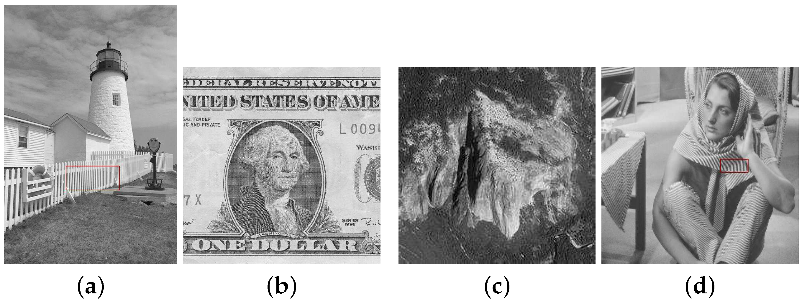
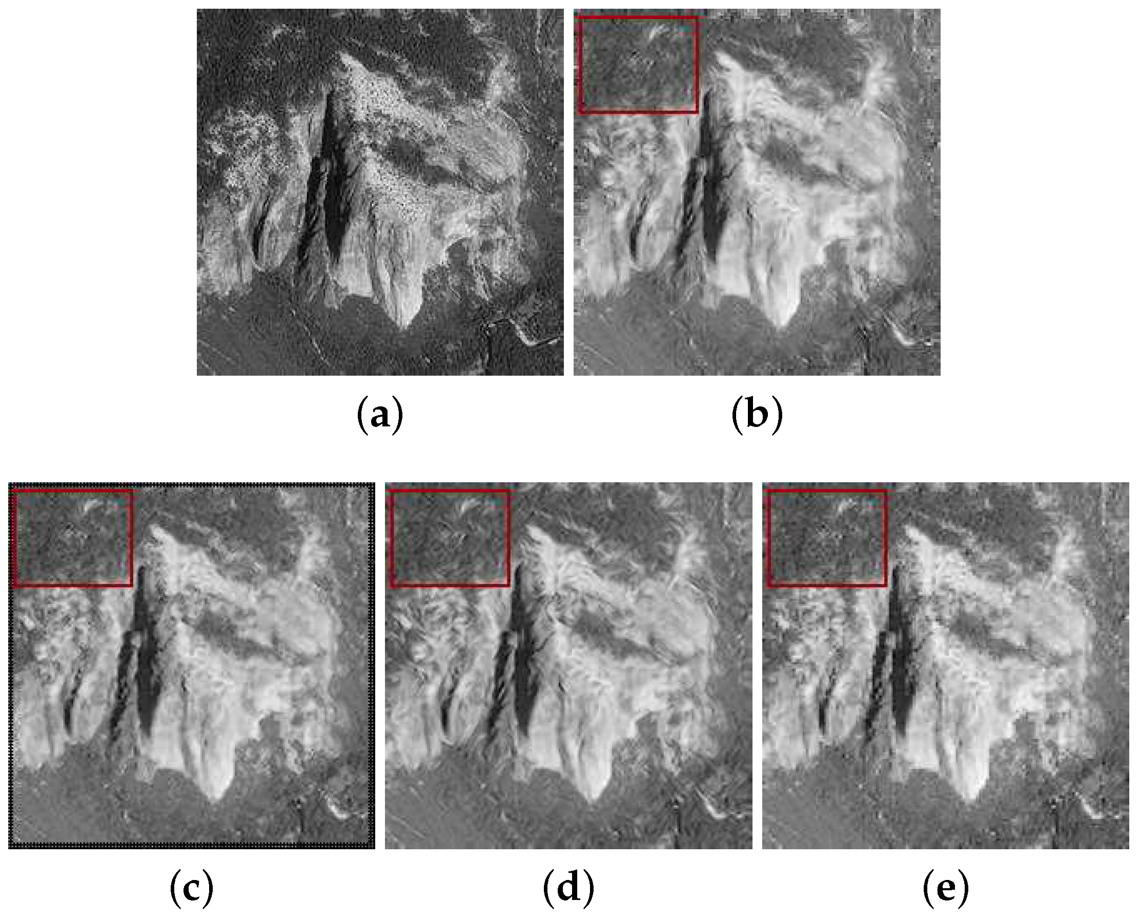
Experiments were conducted to evaluate the effectiveness of the interpolation algorithm. We compare three state-of-the-art interpolation algorithms, including NEDI [6], DFDF [7], SAI [13]. All experiments are performed with software provided by the authors of these algorithms. In our experiments, the four gray images shown in Figure 3 are applied to test visual effects. Table 1 gives the Peak Signal to Noise Ratio (PSNRs) and Structural Similarity Index (SSIMs) generated by all algorithms for the images. It can be seen that the proposed method has a higher average PSNR and SSIM among the compared algorithms.
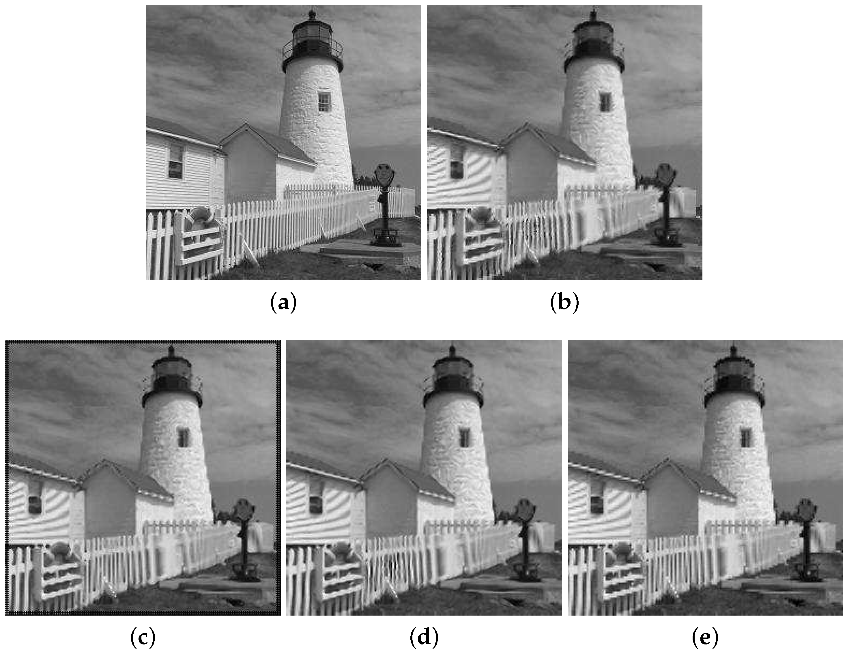
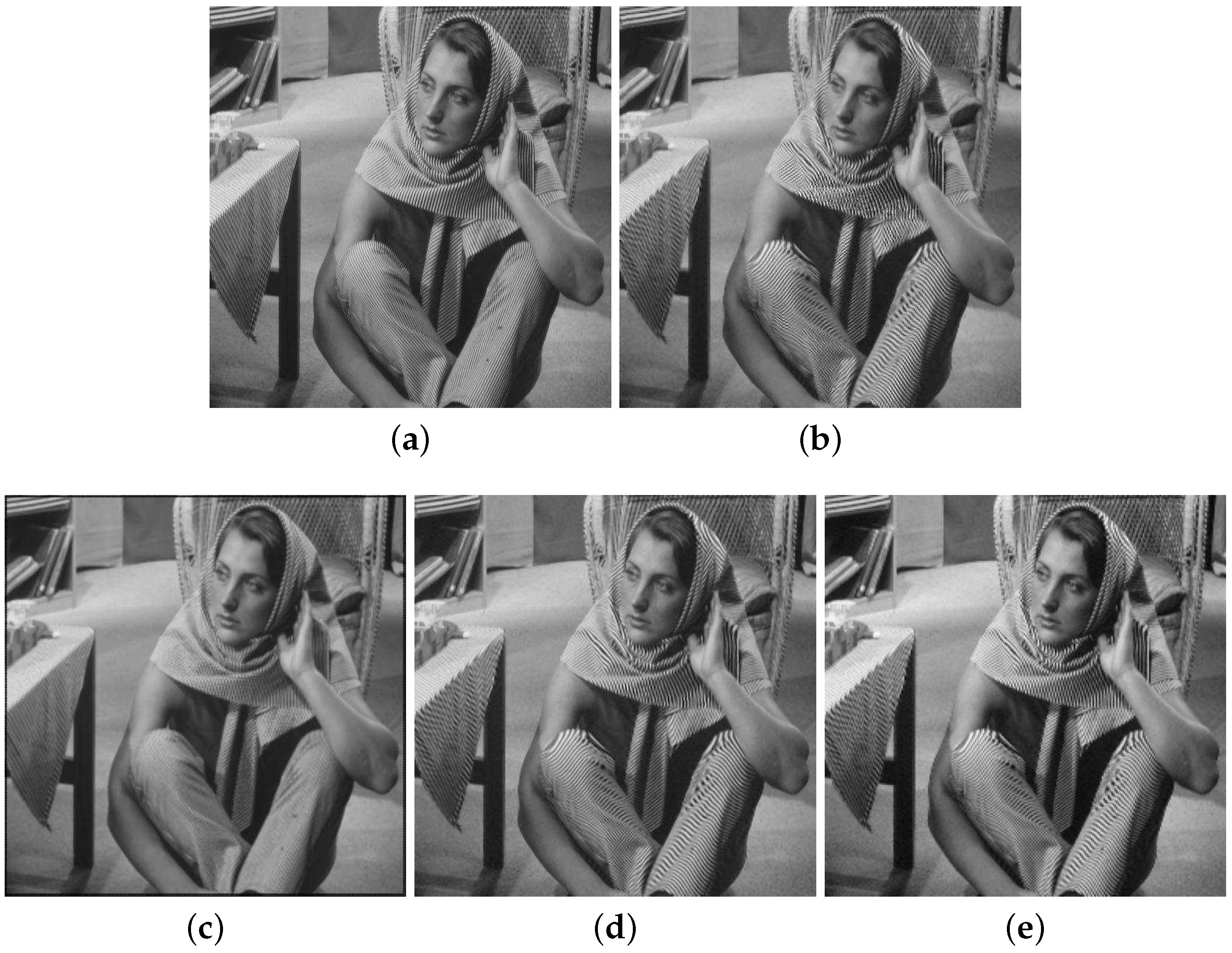
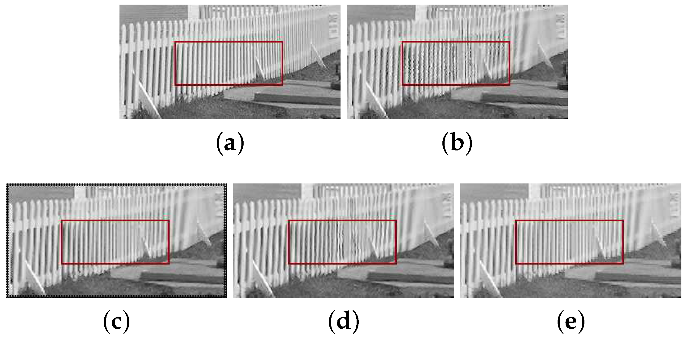
We performed tests on natural images to show the improvements of the proposed method in the visual effects. Figure 4, Figure 5 and Figure 6 show the comparison of interpolation in test images. In Figure 5, all of the interpolation algorithms had aliasing in texture, but our method gave less. In Figure 6, we can see that NEDI suffers from some noisy interpolation artifacts. The SAI method also suffers from noisy artifacts. Our method had better performance in maintaining image features. As shown in Figure 7 and Figure 8, shape loss and noisy points. were introduced in images of a door and fence by the use of NEDI and SAI. The DFDF algorithm also introduced some errors of edge and texture. In general, experimental results on benchmark test images demonstrate that the proposed method achieved very competitive performance with the state-of-art interpolation algorithms, especially in image details and texture features.

5. Conclusions

Although image interpolation is not the most advanced research subject, research results in this field have come forth continuously in recent years. They are usually based on relatively simple theory and have broad applicability However, the interpolation expression forms are various. Therefore, according to the advantages of the different interpolation methods, we can take advantage of these methods and get good results. However, these combination methods have complicated forms, and do not meet the needs of timeliness and practicality. Basically, these methods often neglect the natural image attributes. The main contributions of our method are not combination, but adopting function constructed in Section 2. In this process, non-smooth area detection, image interpolation in different regions, and visual perception are merged into one interpolation function model. The image details and texture features are preserved by using this algorithm, and it can help to describe the image more objectively; hence, more features of the image can be preserved.

Acknowledgments

This work was supported by National Natural Science Foundation of China (No. 61373080,61672018), the Fostering Project of Dominant Discipline and Talent Team of Shandong Province Higher Education Institutions and Natural Science Foundation of Shandong Province (No. ZR2015AM007).

Author Contributions

Xunxiang Yao and Yunfeng Zhang conceived and designed the experiments; Fangxun Bao performed the experiments; Caiming Zhang analyzed the data; Fangxun Bao contributed analysis tools; Xunxiang Yao wrote the paper.

Conflicts of Interest

The authors declare no conflict of interest.

References

  1. Wu, J.; Anisetti, M.; Wu, W.; Damiani, E.; Jeon, G. Bayer demosaicking with polynomial interpolation. J. IEEE Trans. Image Process. 2016, 25, 5369–5382. [Google Scholar] [CrossRef]
  2. Pan, H.; Zou, Z.; Zhang, G.; Zhu, X. A penalized spline-based attitude model for high-resolution satellite imagery. J. IEEE Trans. Geosci. Remote Sens. 2016, 54, 1849–1959. [Google Scholar] [CrossRef]
  3. Su, D.; Willis, P. Image interpolation by pixel-level data-dependent triangulation. Comput. Graph. Forum 2004, 23, 189–201. [Google Scholar] [CrossRef]
  4. Keys, R.G. Cubic convolution interpolation for digital image processing. IEEE Trans. Acoust. Speech Signal Process. 1981, 29, 1153–1160. [Google Scholar] [CrossRef]
  5. Hou, H.; Andrews, H. Cubic splines for image interpolation and digital filtering. IEEE Trans. Acoust. Speech Signal Process. 1978, 26, 508–517. [Google Scholar]
  6. Li, X.; Orchard, M.T. New edge-directed interpolation. IEEE Trans. Image Process. 2001, 15, 1521–1527. [Google Scholar]
  7. Zhang, L.; Wu, X. Image interpolation via directional filtering and data fusion. IEEE Trans. Image Process. 2001, 10, 1521–1527. [Google Scholar]
  8. Battiato, S.; Stanco, F. Alz: Adaptive learning for zooming digital images. In Proceedings of the International Conference on Consumer Electronics (ICCE 2007), Las Vegas, NV, USA, 10–14 January 2007.
  9. Takeda, H.; Farsiu, S.; Milanfar, P. Kernel regression for image processing and reconstruction. IEEE Trans. Image Process. 2007, 16, 349–366. [Google Scholar] [CrossRef] [PubMed]
  10. Battiato, S.; Giuffrida, E.U.; Rundo, F. A cellular neural network for zooming digital colour images. In Proceedings of the International Conference on Consumer Electronics (ICCE 2008), Las Vegas, NV, USA, 9–13 January 2008.
  11. Giachetti, A.; Asuni, N. Fast artifacts-free image interpolation. In Proceedings of the 2008 British Machine Vision Conference, Leeds, UK, 4–9 September 2008.
  12. Asuni, N.; Giachetti, A. Accuracy improvements and artifacts removal in edge based image interpolation. In Proceedings of the 3rd International Conference on Computer Vision Theory and Applications, Funchal, Portugal, 1 July 2008.
  13. Zhang, X.; Wu, X. Image interpolation by adaptive 2-d autoregressive modeling and soft-decision estimation. IEEE Trans. Image Process. 2008, 17, 887–896. [Google Scholar] [CrossRef] [PubMed]
  14. Liu, X.; Zhao, D.; Xiong, R.; Ma, S.; Gao, W.; Sun, H. Image interpolation via regularized local linear regression. IEEE Trans. Image Process. 2011, 20, 3455–3469. [Google Scholar] [PubMed]
  15. Jeong, S.; Yoon, I.; Jeon, J.; Paik, J. Multi-frame example-based super-resolution using locally directional self-similarity. In Proceedings of the IEEE International Conference on Consumer Electronics, Las Vegas, NV, USA, 9–12 January 2015; pp. 353–358.
  16. Jha, A.K.; Kumar, A.; Schaefer, G.; Ahad, M.A.R. An adaptive distance-based edge preserving interpolation algorithm for natural images. In Proceedings of the 2015 IEEE International Conference on Informatics, Electronics and Vision, Fukuoka, Japan, 15–18 June 2015.
  17. Jensen, K.; Anastassiou, D. Subpixel edge localization and the interpolation of still images. IEEE Trans. Image Process. 1995, 4, 285–295. [Google Scholar] [CrossRef] [PubMed]
  18. Carrato, S.; Tenze, L. A high quality 2 x image interpolator. IEEE Signal Process. Lett. 2000, 7, 132–135. [Google Scholar] [CrossRef]
  19. Woods, J.W. Two-dimensional discrete markovian fields. IEEE Trans. Inf. Theory 1972, 18, 232–240. [Google Scholar] [CrossRef]
  20. Said, A.; Pearlman, W.A. A new, fast and efficient image codec based on set partitioning of hierarchical trees. IEEE Trans. Circuits Syst. Video Technol. 1996, 6, 243–250. [Google Scholar] [CrossRef]
  21. Nyiri, E.; Gibaru, O.; Auquiert, P. Fast L1-ck polynomial spline interpolation algorithm with shape-preserving properties. Comput. Aided Geom. Des. 2011, 28, 65–74. [Google Scholar] [CrossRef]
  22. Zhu, C.; Wang, R.; Shi, X.; Liu, F. Functional splines with different degrees of smoothness and their applications. Comput. Aided Des. 2008, 40, 616–624. [Google Scholar] [CrossRef]
  23. Wang, R.; Lang, F. Special multivariate quadratic spline space. Math. Comput. Model. 2009, 49, 760–769. [Google Scholar] [CrossRef]
  24. Duan, Q.; Zhang, Y.; Twizell, E. A bivariate rational interpolation and the properties. Appl. Math. Comput. 2006, 179, 190–199. [Google Scholar] [CrossRef]
  25. Zhang, Y.; Duan, Q.; Twizell, E. Convexity control of a bivariate rational interpolating spline surfaces. Comput. Graph. 2007, 31, 679–687. [Google Scholar] [CrossRef]
  26. Duan, Q.; Bao, F.; Zhang, Y. Shape control of a bivariate interpolating spline surface. Int. J. Comput. Math. 2008, 85, 813–825. [Google Scholar] [CrossRef]
  27. Zhang, Y.; Bao, F.; Zhang, C.; Qi, D. A weighted bivariate blending rational interpolation function and visualization control. J. Comput. Anal. Appl. 2012, 14, 1303–1321. [Google Scholar]
  28. Zhang, Y.; Bao, F.; Zhang, C.; Duan, Q. Local shape control of a bivariate rational interpolating surface with mixing conditions. In Proceedings of the 2011 Eighth International Symposium on Voronoi Diagrams in Science and Engineering (ISVD), Qing Dao, China, 28–30 June 2011; pp. 200–205.
  29. Sun, Q.; Bao, F.; Zhang, Y.; Duan, Q. A bivariate rational interpolation based on scattered data on parallel lines. J. Vis. Commun. Image Represent. 2013, 24, 75–80. [Google Scholar] [CrossRef]
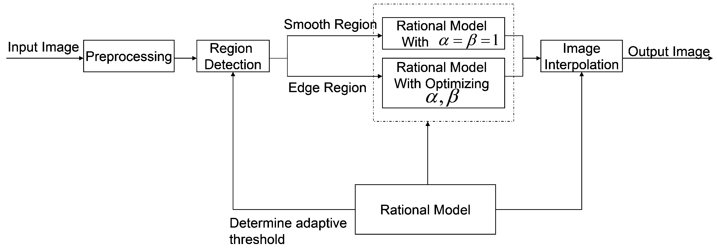
Figure 1. Algorithm framework.
Mca 21 00048 g001
Figure 2. Region detection. (a) Original image; (b) Non-smooth areas.
Mca 21 00048 g002
Figure 3. Images used for quantitative comparison. (a) Light-tower; (b) Dollar; (c) Cliff; (d) Barbara.
Mca 21 00048 g003
Figure 4. (a) Original Image; (b) NEDI; (c) DFDF; (d) SAI; (e) Proposed Method.
Mca 21 00048 g004
Figure 5. (a) Original Image; (b) NEDI; (c) DFDF; (d) SAI; (e) Proposed Method.
Mca 21 00048 g005
Figure 6. (a) Original Image; (b) NEDI; (c) DFDF; (d) SAI; (e) Proposed Method.
Mca 21 00048 g006
Figure 7. (a) Original Image; (b) NEDI; (c) DFDF; (d) SAI; (e) Proposed Method.
Mca 21 00048 g007
Figure 8. (a) Original Image; (b) NEDI; (c) DFDF; (d) SAI; (e) Proposed Method.
Mca 21 00048 g008
Table 1. Peak Signal to Noise Ratio (PSNR) and Structural Similarity Index (SSIM)  results of the reconstructed high-resolution (HR)  images by different methods.
NEDIDFDFSAIOur Method
PSNRSSIMPSNRSSIMPSNRSSIMPSNRSSIM
Light-tower22.780.793723.250.797122.860.800523.370.8009
Dollar19.100.808419.210.806619.240.805519.360.8118
Cliff25.080.711525.050.718425.160.723325.220.7268
Barbara22.350.851323.640.876623.540.863524.120.8801
Milkdrop30.970.915634.360.919632.390.917634.480.9216
Couple28.650.939129.060.941329.320.944329.140.9420
Goldhill26.600.764526.690.767826.920.777226.920.7750
Door33.120.944633.080.944731.160.946733.200.9478
Sky28.410.915428.950.860829.050.936428.960.9378
Boat25.820.894125.540.837825.430.912025.610.8973
Average25.220.820725.740.822525.580.832625.980.8384
NEDI: new edge-directed interpolation; SAI: a soft-decision estimationtechnique for adaptive image interpolation; DFDF: directional filtering and data fusion.