Article

VRP-GMRES(m) Iteration Algorithm for Fast Multipole Boundary Element Method

College of Science, Yanshan University, Qinhuangdao 066004, Hebei, China
*
Author to whom correspondence should be addressed.
Math. Comput. Appl. 2016, 21(4), 49; https://doi.org/10.3390/mca21040049
Submission received: 10 October 2016 / Revised: 22 November 2016 / Accepted: 28 November 2016 / Published: 13 December 2016
(This article belongs to the Special Issue Information and Computational Science)

Abstract

:
To solve large scale linear equations involved in the Fast Multipole Boundary Element Method (FM-BEM) efficiently, an iterative method named the generalized minimal residual method (GMRES(m)) algorithm with Variable Restart Parameter (VRP-GMRES(m)) algorithm is proposed. By properly changing a variable restart parameter for the GMRES(m) algorithm, the iteration stagnation problem resulting from improper selection of the parameter is resolved efficiently. Based on the framework of the VRP-GMRES(m) algorithm and the relevant properties of generalized inverse matrix, the projection of the error vector r m + 1 on r m is deduced. The result proves that the proposed algorithm is not only rapidly convergent but also highly accurate. Numerical experiments further show that the new algorithm can significantly improve the computational efficiency and accuracy. Its superiorities will be much more remarkable when it is used to solve larger scale problems. Therefore, it has extensive prospects in the FM-BEM field and other scientific and engineering computing.

1. Introduction

Mathematical models of partial differential equations are usually established for many problems in scientific and engineering fields. After discretization, the equations can be concluded as the solution of a large scale linear system of equations, which can be expressed as
A x = b , A R n × n , x , b R n ,
where the coefficient matrix A is nonsingular. The generalized minimal residual (GMRES(m)) algorithm based on the Galerkin principle is the most successful method to solve Equation (1). At present, it has served as the fast solver for the Fast Multipole Boundary Element Method (FM-BEM). FM-BEM is a combination of the fast multipole expansion method (FMM) and the traditional boundary element method (BEM). FMM was first proposed by Greengard and Rokhlin [1,2] to accelerate the evaluation of interactions of large ensembles of particles governed by the Laplace’s equation. The main idea behind the FMM is a multipole expansion of the kernel in which the connection between the collocation point and the source point is separated. Many research works have been published since then to improve and extend the applicability of the FMM [3,4,5,6,7]. Recently, Gu and Chen [8,9] applied the FMM to accelerate the solutions of the regularized meshless method (RMM) for large-scale three-dimensional elasticity problems and extended the singular boundary method (SBM) for the solution of 3D problems in linear elasticity. With the FMM and iterative solver GMRES(m), we are able to construct the FM-BEM. In the last several decades, the FM-BEM has been developed and used successfully for solving many large-scale applied mechanics problems. Shen and Liu put forward an adaptive fast multipole boundary element method for three-dimensional acoustic wave problems [10]; Wang and Yao came up with a new version of FMM for the numerical analysis of mechanical properties in 3D particle reinforced composites [11]; Gui and Huang presented an optimization FMM-BEM for a 3D Elastic Problem [12] and more work on these topics can be found in References [13,14,15]. In addition, the GMRES(m) algorithm has become the research focus in many fields [16,17,18]. Recent computations showed that it was very effective when the coefficient matrix A was well-conditioned or not severely ill-conditioned [19,20]. Otherwise preconditioned techniques must be applied [21,22,23,24].
For the GMRES(m) algorithm, the selected parameter m is fixed during the whole iterative process; therefore, the selection of m is one of the key factors for the algorithm implementation. Research shows that a small value of m may result in slow convergence or no convergence, while a large value of m will cause too much of a memory requirement. Therefore, it is a difficult problem for many scholars to properly select the parameters m. Recently, some researchers have tried to overcome these difficulties by changing the restart parameter m in the GMRES(m) algorithm. Baker tried to improve the convergence by selecting an arbitrary parameter m. In addition, he tried it by determining the parameter m according to the residual vector norm ratio of two successive iterations [25,26,27]. However, the effect was not so good. Peairs determined the value of m by a reinforcement learning method, which indicated that proper changing of m could improve the computational efficiency. However, it was only a kind of machine learning method. Thus, it had certain limitations [28].
In this paper, the GMRES(m) algorithm combined with the FM-BEM is studied, and a new kind of GMRES(m) algorithm with Variable Restart Parameter (VRP-GMRES(m) algorithm) is presented. By appropriately changing a variable restart parameter, the new algorithm can effectively avoid many disadvantages caused by improper selection of parameter m in the GMRES(m) algorithm. At the same time, the computational efficiency and accuracy will be greatly improved.

2. Fundamental Theory for the GMRES(m) Algorithm

2.1. Galerkin Principle

Give an arbitrary initial value x 0 R n . Let x = x 0 + z , and then Equation (1) is equivalent to
A z = r 0 ,
where r 0 = b A x 0 indicates the initial residual vector. Suppose that K m and L m are two m-dimensional Krylov subspaces in R n , and they are formed by
K m = s p a n r 0 , A r 0 , , A m 1 r 0 ,
L m = s p a n A r 0 , A 2 r 0 , , A m r 0 = A K m .
Let v 1 , v 2 , , v m and w 1 , w 2 , , w m be the bases of K m and L m , respectively; V m = v i i = 1 m and W m = w i i = 1 m . For the solution of Equation (2) , the Galerkin principle can be described as follows: give a fixed m > 0 , and find an approximate solution z m K m , so that ( r 0 A z m ) L m , namely, ( r 0 A V m y m ) L m or ( r 0 A V m y m , w i ) = 0 , y m R m .

2.2. Arnoldi Process

The Arnoldi process can be described as follows:
  • For the given m > 0 and x 0 R n , compute v 1 = r 0 r 0 r 0 r 0 , r 0 = b A x 0 .
  • When k = 1 , 2 , , m , compute v ¯ k + 1 = A v k i = 1 k h i , k v i , h i , k = A v k , v i and h k + 1 , k = v ¯ k + 1 , respectively. It is obvious that v ¯ k + 1 v i i = 1 , 2 , , k .
  • If h k + 1 , k = 0 , then v k + 1 = 0 and stop calculation. Otherwise, let v k + 1 = v ¯ k + 1 v ¯ k + 1 h k + 1 , k h k + 1 , k .
The Arnoldi process has the following important property:
Theorem 1.
In the Arnoldi process, let V m + 1 = ( V m v m + 1 ) and H ¯ m = H m h m + 1 , m e m T , and then we have the following relationship [28]:
A V m = V m H m + h m + 1 , m v m + 1 e m T , A V m = V m + 1 H ¯ m , V m + 1 T V m + 1 = I ,
where H m = ( h i j ) m is an upper Hessenberg matrix, e m T = ( 0 , 0 , , 1 ) R m , and I is an m + 1 order identity matrix.

2.3. GMRES(m) Algorithm

Theorem 2.
Suppose that A R n × n and L m = A K m , x = x 0 + z = x 0 + V m y . Then, the approximate solution z m obtained from the Galerkin principle makes the residual r 0 A z be at a minimum in the Krylov subspace K m , and the residual satisfies [29]
r = b A x = r 0 A z = β e 1 H ¯ m y ,
where β = r 0 , e 1 = ( 1 , 0 , , 0 ) T R m + 1 .
Theorem 2 indicates that min z m K m r 0 A z m = min y R m β e 1 H ¯ m y . The basic thought of the GMRES(m) algorithm is to give a fixed restart parameter m and compute z m by an iterative procedure so that r m = r 0 A z m < ε , ε > 0 .
The GMRES(m) algorithm includes the following steps:
  • Give a fixed integer m < < n and an initial value x ( 0 ) R n , compute r ( 0 ) = b A x ( 0 ) , and let r 0 = r ( 0 ) .
  • Obtain v i i = 1 m and H ¯ m through the Arnoldi process.
  • Solve the least squares problem
    min y R m β e 1 H ¯ m y
    to obtain y m , where e 1 = 1 , 0 , , 0 T R m + 1 . Then, compute z m = V m y m .
  • Form an iterative process x ( k + 1 ) = x ( k ) + z m or r ( k + 1 ) = r ( k ) A z m , k = 0 , 1 , 2 , .
  • If r ( k + 1 ) < ε , then x * x k + 1 and stop calculation. Otherwise, let r 0 = r ( k + 1 ) , and go to 2.
For the GMRES(m) algorithm, arbitrary selection of parameter m cannot guarantee convergence. In fact, appropriate change of m can effectively improve the convergence and avoid the phenomenon of slow convergence or even no convergence.

3. VRP-GMRES(m) Iterative Algorithm and Convergence Analysis

3.1. VRP-GMRES(m) Algorithm

The basic thought of the VRP-GMRES(m) algorithm is to appropriately change the restart parameter m and carry out iterative procedures so that the residual vector satisfies r m = r 0 A z m < ε , ε > 0 . It includes the following main steps:
  • Give an integer m < < n and an initial value x ( 0 ) R n , compute r ( 0 ) = b A x ( 0 ) , and let r 0 = r ( 0 ) .
  • Carry out the Arnoldi process and obtain v i i = 1 m and H ¯ m .
  • Solve the least squares problem
    min y R m β e 1 H ¯ m y
    and get y m . Then, compute z m = V m y m .
  • Form an iterative process by x ( k + 1 ) = x ( k ) + z m , k = 0 , 1 , 2 , Compute r ( k + 1 ) = b A x ( k + 1 ) .
  • If r ( k + 1 ) < ε . Then, x * x k + 1 and stop. If r ( k + 1 ) ε , then let r 0 = r ( k + 1 ) , m = m + 1 , and go to 2.
For the VRP-GMRES(m) algorithm, slow convergence or no convergence rarely occurs. However, the memory requirement will grow with the increase of parameter m , which can be cleverly avoided. When m increases to some extent and the residual norm reduces to a proper value, the parameter m can be fixed and the GMRES(m) algorithm will be carried out.

3.2. Convergence Analysis

Definition 1.
Suppose that A C m × n , X C m × n , at the same time if
A X A = A , X A X = X , ( A X ) H = A X , ( X A ) H = X A ,
then X is the pseudo inverse matrix of A, denoted A + , namely X = A + [30].
Theorem 3.
Suppose that A C m × n , and A = B C is the maximum rank decomposition of A, then X = C H ( C C H ) 1 ( B H B ) 1 B H is the pseudo inverse matrix of A.
Proof of Theorem 3.
A X A = B C C H ( C C H ) 1 ( B H B ) 1 B H B C = B C = A ,
X A X = C H ( C C H ) 1 ( B H B ) 1 B H B C C H ( C C H ) 1 ( B H B ) 1 B H = C H ( C C H ) 1 ( B H B ) 1 B H = X .
Hereto, the first two Moore Penrose equations are established. The following is to verify the other two Moore Penrose equations:
( A X ) H = [ B C C H ( C C H ) 1 ( B H B ) 1 B H ] H = [ B ( B H B ) 1 B H ] H = B ( B H B ) 1 B H = A X ,
( X A ) H = [ C H ( C C H ) 1 ( B H B ) 1 B H B C ] H = [ C H ( C C H ) 1 C ] H = C H ( C C H ) 1 C = X A ,
From Definition 1, the matrix X is a pseudo inverse matrix of A.  ☐
Corollary 1.
Suppose that A C m × n is a matrix with full column rank. Then, we have
A + = A H A 1 A H .
Theorem 4.
Suppose that r m and r m + 1 are the error vector of the m cycle and m + 1 , respectively. Then, the following relationship is established:
cos r m , r m + 1 = r m + 1 2 r m 2 .
Proof of Theorem 4.
For the VRP-GMRES(m) algorithm, when m = m + 1 , the subspace K m becomes
K m + 1 = s p a n r m , A r m , , A m r m .
From the Arnoldi process, v i i = 1 m + 1 and H ¯ m + 1 are obtained, where v 1 = r m β , β = r m 2 , cos r m , r m + 1 = cos v 1 , r m + 1 = v 1 T r m + 1 r m + 1 2 .
From Equation (5), the least squares solution y m + 1 = H ¯ m + 1 + β e 1 , e 1 R m + 2 is obtained, where H ¯ m + 1 + is a real matrix with full column rank. According to Equation (6), we have
H ¯ m + 1 + = H ¯ m + 1 T H ¯ m + 1 1 H ¯ m + 1 T .
Then,
y m + 1 = H ¯ m + 1 T H ¯ m + 1 1 H ¯ m + 1 T β e 1 , e 1 R m + 2 .
On the other hand, we have
r m + 1 = b A x m + 1 = b A x m + V m + 1 y m + 1 = r m A V m + 1 y m + 1 .
Accrording to Equation (3), we have A V m + 1 = V m + 2 H ¯ m + 1 . Then, we have
r m + 1 = r m V m + 2 H ¯ m + 1 y m + 1 = β v 1 V m + 2 H ¯ m + 1 y m + 1 .
Thus,
r m + 1 2 2 = ( β v 1 V m + 2 H ¯ m + 1 y m + 1 ) T ( β v 1 V m + 2 H ¯ m + 1 y m + 1 ) = β 2 β v 1 T V m + 2 H ¯ m + 1 y m + 1 β y m + 1 T H ¯ m + 1 T V m + 2 T v 1 + y m + 1 T H ¯ m + 1 T V m + 2 T V m + 2 H ¯ m + 1 y m + 1 = β 2 β h T y m + 1 ( β y m + 1 T H ¯ m + 1 T V m + 2 T v 1 β y m + 1 T H ¯ m + 1 T V m + 2 T V m + 2 H ¯ m + 1 H ¯ m + 1 T H ¯ m + 1 1 H ¯ m + 1 T e 1 ) = β 2 β h T y m + 1 = β ( β h T y m + 1 ) .
At the same time,
v 1 T r m + 1 = v 1 T ( β v 1 V m + 2 H ¯ m + 1 y m + 1 ) = β h T y m + 1
( h T indicates a vector formed by the first line elements in H ¯ m + 1 ), follows
c o s r m , r m + 1 = β h T y m + 1 β ( β h T y m + 1 ) = r m + 1 2 r m 2 .
Theorem 5.
For the VRP-GMRES(m) algorithm, let E = r m 2 , E ¯ = r m + 1 2 , and therefore E ¯ < E .
Proof of Theorem 5.
In Equation (8), cos r m , r m + 1 1 , namely,
r m + 1 2 r m 2 1 .
Because h T y m + 1 0 , it follows
E ¯ = r m + 1 2 < r m 2 = E .

4. Numerical Experiments

In this section, three different types of numerical experiments are given to illustrate the validity and feasibility of the VRP-GMRES(m) algorithm. In Example (1) and Example (2), take x ( 0 ) = ( 0 , 0 , , 0 ) T R ( n 1 ) 2 as the initial value and ε = 1 × 10 8 as the convergence criterion.
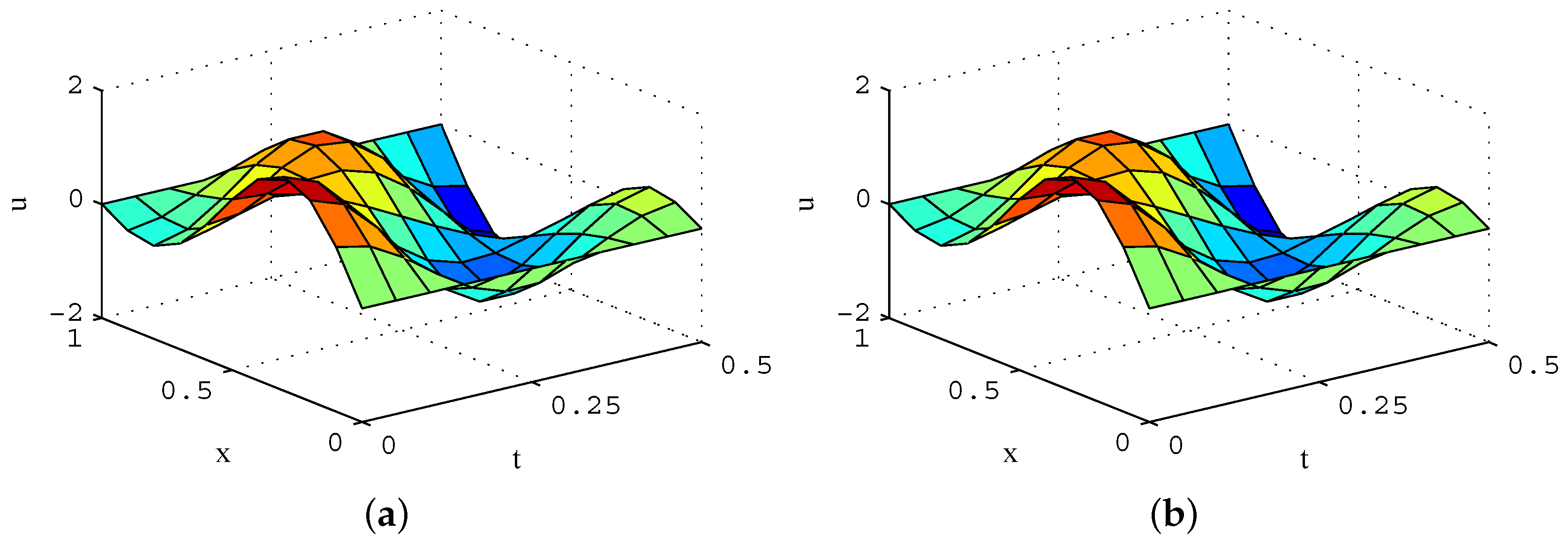
Example 1.
Consider the following one-dimensional Wave equation:
u t t = 4 u x x , 0 < x < 1 , 0 < t < 0 . 5 , u 0 , t = u 1 , t = 0 , 0 t 0 . 5 , u x , 0 = f x = sin π x + sin 2 π x , 0 x 1 , u t x , 0 = g x = 0 , 0 x 1 .
As is shown in Figure 1a, the exact solution is u x , t = sin π x cos 2 π t + sin 2 π x cos 4 π t , where u x , t indicates the amplitude. For the problem expressed by Equation (10), n equall divisions along the x-direction and t-direction can be obtained by the central difference method.
A x = b , A R n 1 2 × n 1 2 , x , b R ( n 1 ) 2 .
Equation (11) is solved by the VRP-GMRES(m) algorithm, and the numerical results are shown in Figure 1b. From Figure 1, the numerical solution is consistent with the exact solution.
Equation (
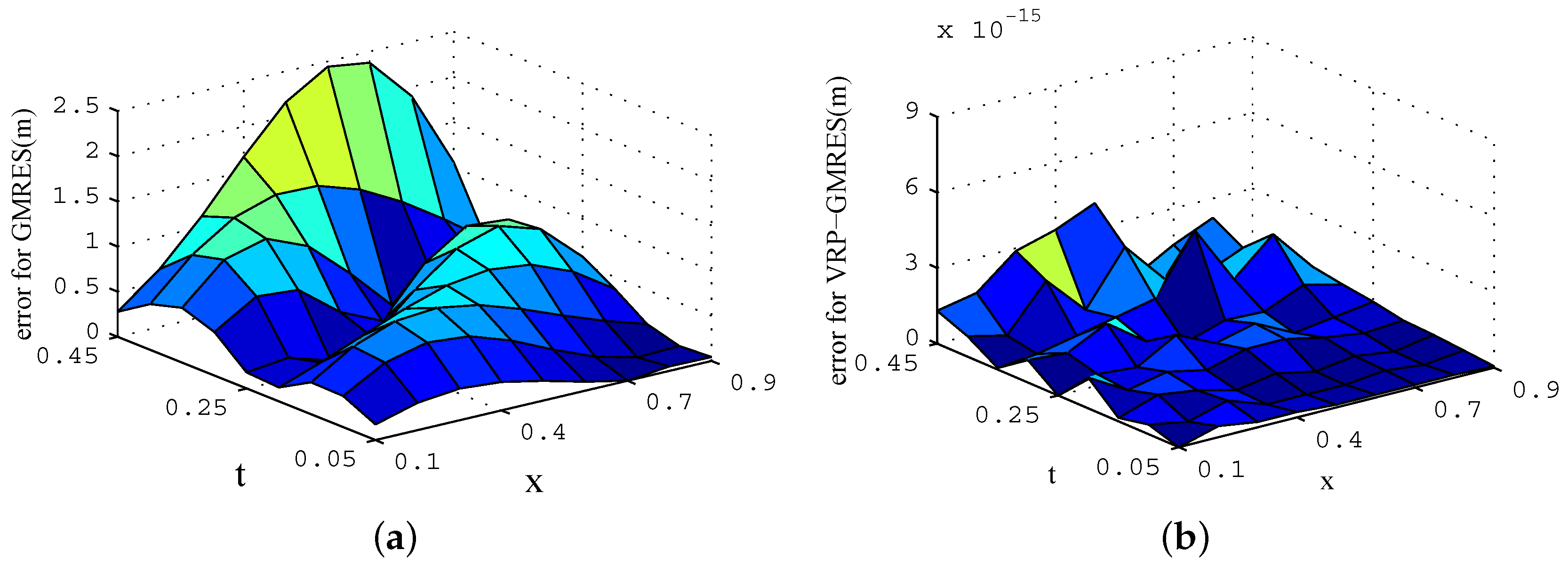
11) is solved by the GMRES(m) algorithm and VRP-GMRES(m) algorithm, respectively. When n = 10 , m = 7 , the condition number is 56.5079. For the GMRES(m) algorithm, iterative stagnation occurs after 9 iterations, and the residual norm is 1.4099. However, for the VRP-GMRES(m) algorithm, the residual norm has reduced to 1.4230 × 10 14 after only 3 iterations, as is shown in 
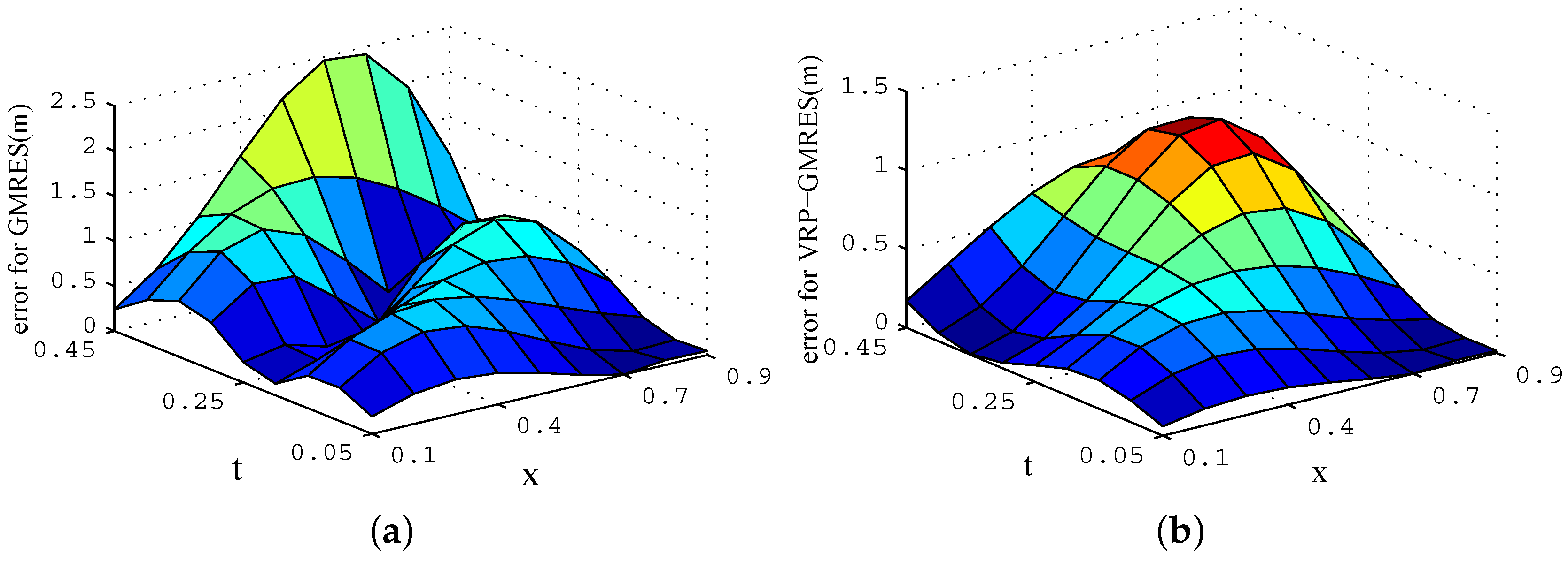
Figure 2. The comparison of absolute errors in the iterative process is shown in Figure 2 and Figure 3.
From Figure 2 and Figure 3, for the same number of iterations, we can see that the absolute errors generated from the VRP-GMRES(m) algorithm are much smaller than those from the GMRES(m) algorithm. With the increase in the number of iterations, the errors from the VRP-GMRES(m) algorithm reduces much faster. It shows that the new algorithm not only has higher computational accuracy, but can also speedily converge.
The parameters n and m are taken as different values and the calculation results from the two algorithms are compared. Table 1, Table 2, Table 3 and Table 4 show the iteration times, computation time, computational accuracy and convergence, respectively. From Table 1, Table 2 and Table 3, we can see that the new algorithm is fast convergent, stable, highly accurate and effective. From Table 1, Table 2, Table 3 and Table 4, the selection of parameter m is very important for the GMRES(m) algorithm, and larger or smaller value of m will result in an algorithm failure. However, it has no effect on the VRP-GMRES(m) algorithm because the variable restart parameter m can partly reduce the sensitivity of m.
In fact, the condition number of coefficient matrix A keeps growing with the increase of n. When n = 60 , it reaches 2.1098 × 10 3 , which makes Equation (11) become severely ill-conditioned. From Table 1, under the same accuracy, the number of iterations for the GMRES(m) algorithm is 11.7 times larger than that for the VRP-GMRES(m) algorithm, and the computation time is 10.7 times larger. With the increase of computing scale, the VRP-GMRES(m) algorithm will be much more effective, and its engineering application prospect is much wider.
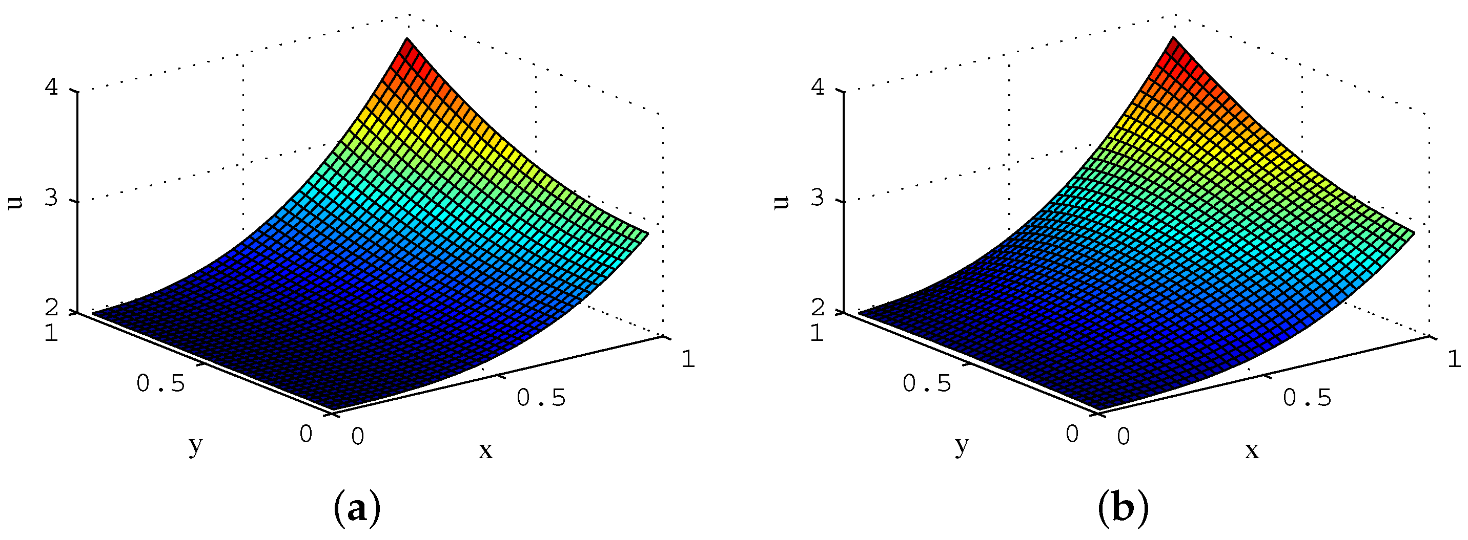
Example 2.
Consider the following two-dimensional Poisson equation:
u x x + u y y = 2 3 x + x 2 + y 2 , x , y Ω , u x , y = x 2 x + y 2 + 2 , x , y Ω ,
where Ω = ( x , y ) 0 x 1 , 0 y 1 .
The exact solution is u x , y = x 2 x + y 2 + 2 , which indicates a temperature distribution function. The temperature distribution is shown in Figure 4a. For the problem expressed by Equation (12), n equal divisions along the x-direction and t-direction can be obtained by a five-point difference scheme. After discretization, a linear equation can be obtained, which is expressed as follows:
A x = b , A R n 1 2 × n 1 2 , x , b R ( n 1 ) 2 .
Take n = 40 , m = 10 , Equation (13) is solved by the VRP-GMRES(m) algorithm , and the temperature distribution is shown in Figure 4b. From Figure 4, the numerical solution is consistent with the exact solution.
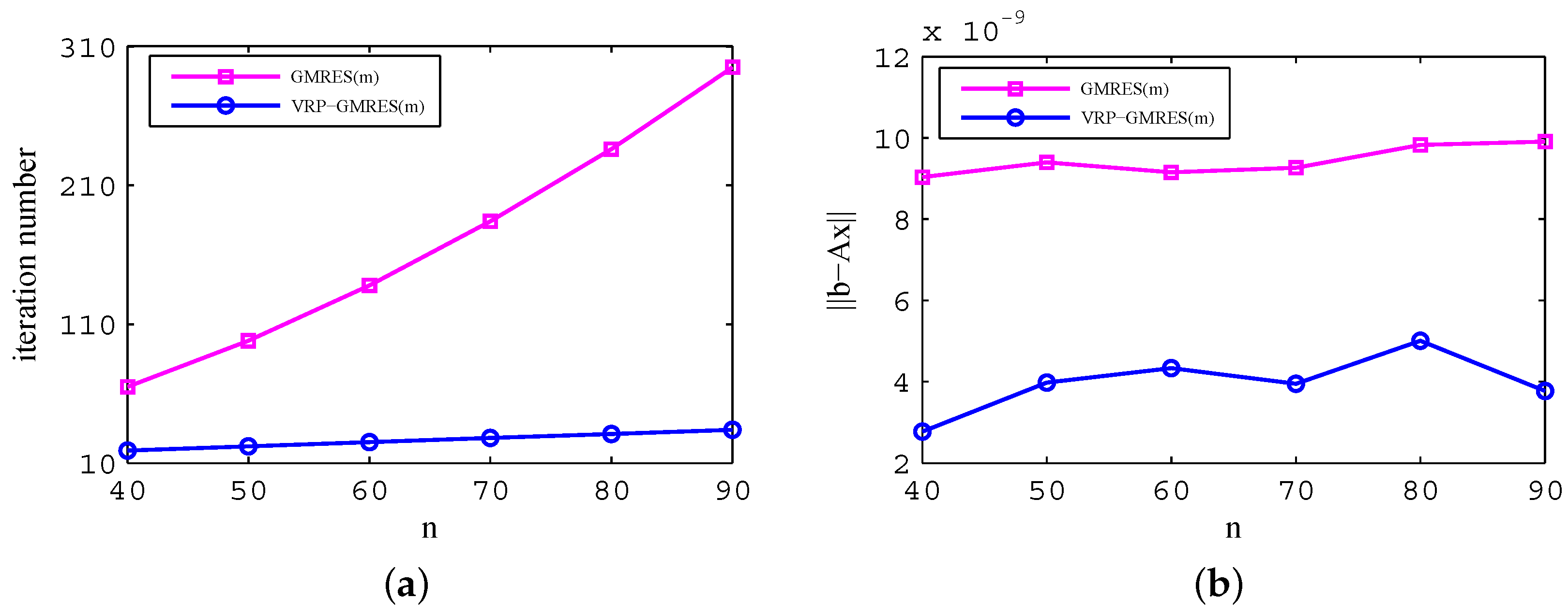
When m = 10 , Equation (13) is solved by the GMRES(m) algorithm and VRP-GMRES(m) algorithm, respectively. With the increase of the computational scale, there are few changes in the iteration times for the VRP-GMRES(m) algorithm, and it is much lower than that for the GMRES(m) algorithm, as shown in Figure 5a. Thus, the new algorithm has higher computational efficiency. At the same time, it has higher computational accuracy, as is shown in Figure 5b. In addition, the total computation time for the VRP-GMRES(m) algorithm is much less than that for the GMRES(m) algorithm, as is shown in Table 5.
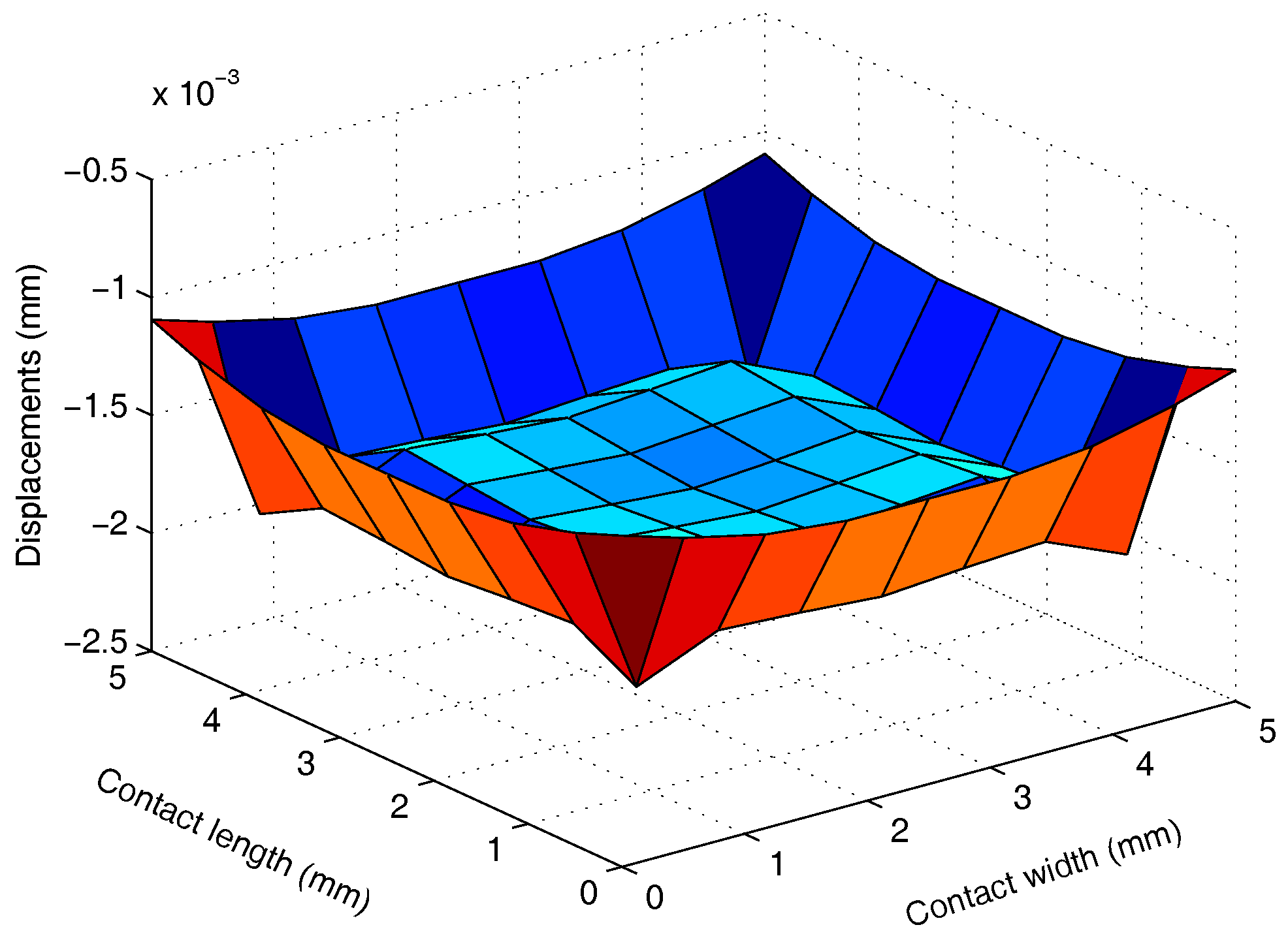
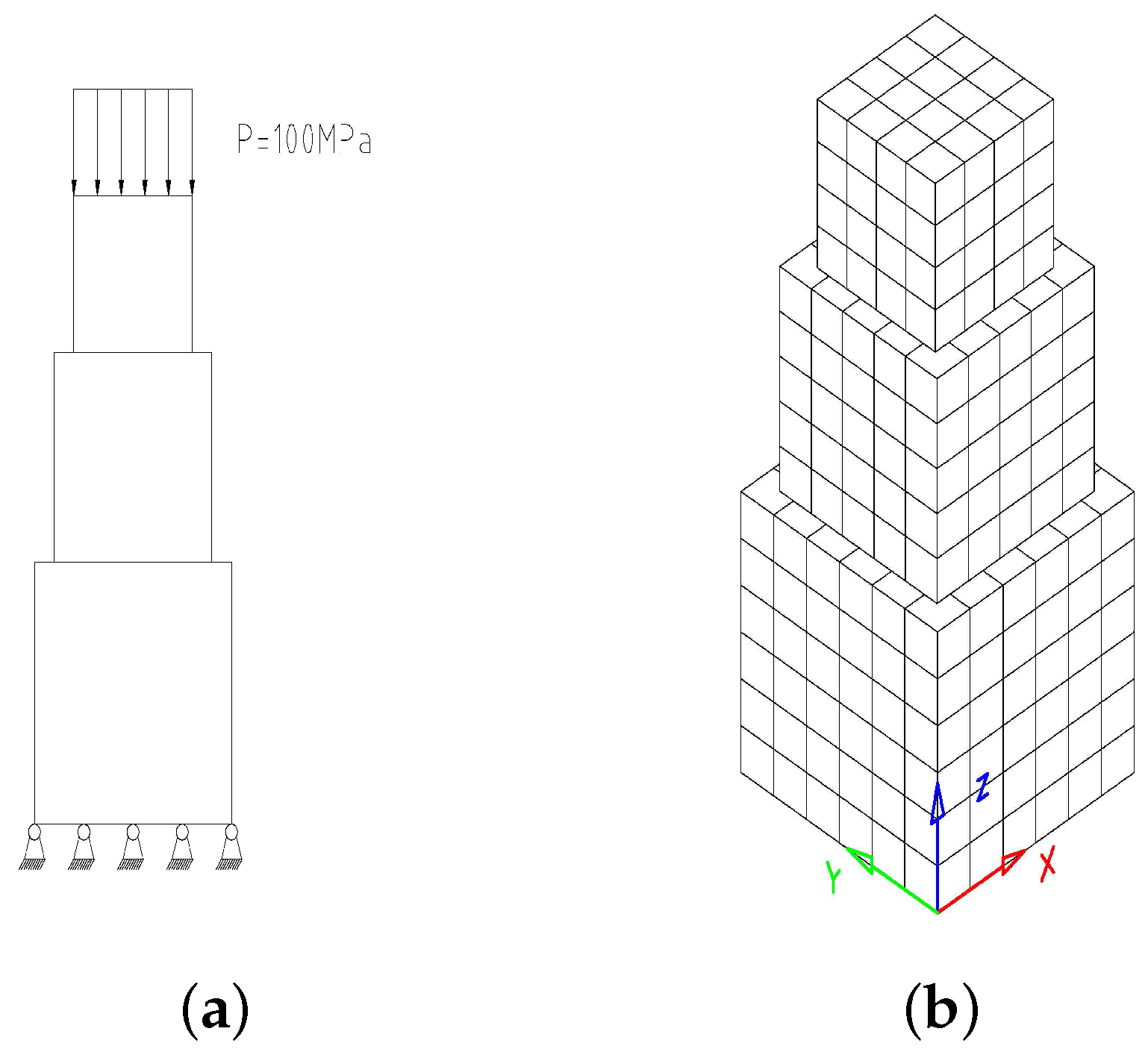
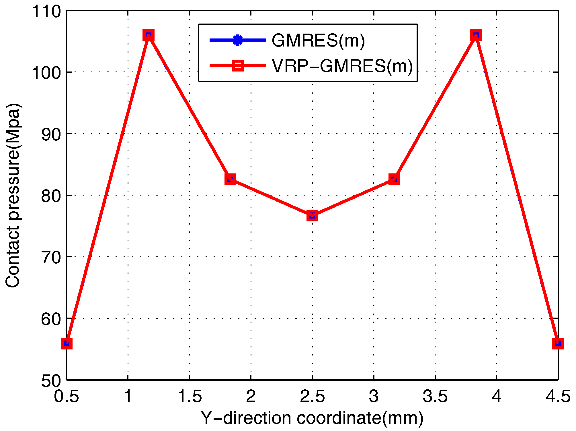
Example 3.
Consider an elastic body A, B, C (with sides of 5 m m , 4 m m , 3 m m ) in contact with each other. The model and the discrete meshes are shown in Figure 6. The discrete data are shown in Table 6. Bodies A, B and C are of the same material with Young modulus E = 210 G P a , Poisson ratio υ = 0.3 , and the friction coefficient f = 0.2 . For body C, a uniform load P = 100 M P a is applied tothe top surface. The total load is divided into six steps, and the contact tolerance is 0.001 m m .
In the example, the VRP-GMRES(m) algorithm is used as a fast solver for the FM-BEM, and some results are shown in Figure 7, which are consistent with those obtained by the GMRES(m) algorithm. The iteration times by the GMRES(m) algorithm and VRP-GMRES(m) algorithm are shown in Table 7. From Table 7, we can see that there are few changes in the iteration times for the VRP-GMRES(m) algorithm. However, the relative error is quite small for the pressure of the same node, as is shown in Figure 8.
From Table 7 and Figure 8 , the VRP-GMRES(m) algorithm is more rapidly and stably convergent than the GMRES(m) algorithm.

5. Conclusions

In this paper, an iterative VRP-GMRES(m) algorithm is proposed for the solution of linear equations, which can be used as an improved solver of the FM-BEM and can be used to solve many mathematical, mechanical, physical and engineering problems. Through theoretical analysis, the new algorithm is proved to be rapidly convergent with higher computational accuracy. Numerical experiments show that the presented algorithm not only has higher computational efficiency and accuracy, but also is much more stable. The results of the last example also prove that it is highly efficient and rapidly convergent for the elastic problems. On the whole, the new algorithm has extensive prospects in the FM-BEM field and other large-scale scientific and engineering computing.

Acknowledgments

This work is supported by National Natural Science Foundation of China (No. 11301459) and Natural Science Foundation of Hebei Province (No. A2015203121).

Conflicts of Interest

The authors declare no conflict interest.

References

  1. Greengard, L.; Rokhlin, V. A fast algorithm for particle simulations. J. Comput. Phys. 2001, 73, 325–348. [Google Scholar] [CrossRef]
  2. Rokhlin, V. A fast algorithm for the discrete Laplace transformation. J. Complex. 1988, 4, 12–32. [Google Scholar] [CrossRef]
  3. White, C.A.; Head-Gordon, M. Derivation and efficient implementation of the fast multipole method. J. Chem. Phys. 1994, 101, 6593–6605. [Google Scholar] [CrossRef]
  4. White, C.A.; Johnson, B.G.; Gill, P.M.W.; Head-Gordon, M. The continuous fast multipole method. Chem. Phys. Lett. 1994, 230, 8–16. [Google Scholar] [CrossRef]
  5. White, C.A.; Head-Gordon, M. Rotating around the quartic angular momentum barrier in fast multipole method calculations. J. Chem. Phys. 1996, 105, 5061–5067. [Google Scholar] [CrossRef]
  6. Beatson, R.; Greengard, L. A Short Course on Fast Multipole Methods. Wavelets Multilevel Methods & Elliptic Pdes; Oxford University Press: Oxford, UK, 1997. [Google Scholar]
  7. Cheng, H.; Greengard, L.; Rokhlin, V. A Fast Adaptive Multipole Algorithm in Three Dimensions. J. Comput. Phys. 1999, 155, 468–498. [Google Scholar] [CrossRef]
  8. Gu, Y.; Chen, W.; Gao, H.; Zhang, C. A meshless singular boundary method for three-dimensional elasticity problems. Int. J. Numer. Methods Eng. 2016, 107, 109–126. [Google Scholar] [CrossRef]
  9. Wang, Z.; Gu, Y.; Chen, W. Fast-multipole accelerated regularized meshless method for large-scale isotropic heat conduction problems. Int. J. Heat Mass Transf. 2016, 101, 461–469. [Google Scholar] [CrossRef]
  10. Shen, L.; Liu, Y.J. An adaptive fast multipole boundary element method for three-dimensional acoustic wave problems based on the Burton-Miller formulation. Comput. Mech. 2007, 12, 554–561. [Google Scholar] [CrossRef]
  11. Wang, H.; Yao, Z. Large Scale Analysis of Mechanical Properties in 3-D Fiber-Reinforced Composites Usinga New Fast Multipole Boundary Element Method. J. Tsinghua Univ. (Sci. Technol.) 2007, 12, 461–472. [Google Scholar]
  12. Wang, H.; Yao, Z. Application of a new fast multipole BEM for simulation of 2D elastic solid with large number of inclusions. Acta Mech. Sin. 2004, 20, 613–622. [Google Scholar]
  13. Liu, Y. Fast Multipole Boundary Element Method: Theory and Applications in Engineering; Cambridge University Press: Cambridge, UK, 2009. [Google Scholar]
  14. Engheta, N.; Murphy, W.D.; Rokhlin, V.; Vassiliou, M.S. The fast multipole method (FMM) for electromagnetic scattering problems. IEEE Trans. Antennas Propag. 1992, 40, 634–641. [Google Scholar] [CrossRef]
  15. Liu, Y.J.; Nishimura, N.; Yao, Z.H. A fast multipole accelerated method of fundamental solutions for potential problems. Eng. Anal. Bound. Elem. 2005, 29, 1016–1024. [Google Scholar] [CrossRef]
  16. Philippeon, B.; Reichel, L. The generation of Krylov subspace bases. Appl. Numer. Math. 2012, 62, 1171–1186. [Google Scholar] [CrossRef]
  17. Luo, D.M.; Chen, P.J.; Wu, X.M. Application of GMRES algorithm to hovering rotor simulation. Kongqi Donglixue Xuebao/Acta Aerodyn. Sin. 2012, 30, 471–476. [Google Scholar]
  18. Dai, Y.Z.; Song, J.Z.; Ren, H.L.; Li, H. Application of GMRES to the hydroelastic analysis of large ofshore structure. Ocean Eng. 2003, 21, 15–22. [Google Scholar]
  19. Pu, B.Y.; Huang, Y.Z.; Wen, C. A preconditioned and extrapolation-accelerated GMRES method for PageRank. Appl. Math. Lett. 2014, 37, 95–100. [Google Scholar] [CrossRef]
  20. Saad, Y.; Schultz, M.H. GMRES a Generalized Minimal Residual Algorithm for Solving Non-symmetric Linear Systems. Siam J. Sci. Stat. Comput. 2006, 7, 856–869. [Google Scholar] [CrossRef]
  21. Ayachour, E.H. A fast implementation for GMRES method. J. Comput. Appl. Math. 2003, 159, 269–283. [Google Scholar] [CrossRef]
  22. Jose, E.P.; Alex, A.P.; Ricardo, P.; Carlos, P.P. Making use of BDE-GMRES methods for solving short and long-term dynamics in power systems. Int. J. Electr. Power Energy Syst. 2013, 45, 293–302. [Google Scholar]
  23. Yin, J.F.; Hayami, K. Preconditione GMRES methods with incomplete Givens orthogonalization method for large sparse least-squares problems. J. Comput. Appl. Math. 2009, 226, 177–186. [Google Scholar] [CrossRef]
  24. Lin, F.R.; Yang, S.W.; Jin, X.Q. Preconditioned iterative methods for fractional diffusion equation. J. Comput. Phys. 2014, 256, 109–117. [Google Scholar] [CrossRef]
  25. Liang, Y.; Szularz, M.; Yang, L.T. Finite-element-wise domain decomposition iterative solvers with polynomial preconditioning. Math. Comput. Model. 2013, 58, 421–437. [Google Scholar] [CrossRef]
  26. Baker, A.H. On Improving the Performance of the Linear Solver Restarted Gmres; University of Colorado at Boulder: Boulder, CO, USA, 2003. [Google Scholar]
  27. Baker, A.H.; Jessup, E.R.; Kolev, T.V. A simple strategy for varying the restart parameter in GMRES(m). J. Comput. Appl. Math. 2009, 230, 751–761. [Google Scholar] [CrossRef]
  28. Peairs, L.; Chen, T.Y. Using reinforcement learning to vary the m in GMRES(m). Procedia Comput. 2011, 4, 2257–2266. [Google Scholar] [CrossRef]
  29. Essai, A. Weighted FOM and GMRES for solving nonsymmetric linear systems. Numer. Algorithms 1998, 18, 227–292. [Google Scholar] [CrossRef]
  30. Cai, D.Y.; Bai, F.S. Advanced Numerical Analysis; Tsinghua University Press: Beijing, China, 1997. [Google Scholar]
Figure 1. Amplitude distribution ( n = 10 , m = 7 ). (a) exact solution; and (b) numerical solution.
Mca 21 00049 g001
Figure 2. Absolute errors after three iterations. (a) generalized minimal residual method (GMRES)(m) algorithm; (b) Variable Restart Parameter(VRP)-GMRES(m) algorithm.
Mca 21 00049 g002
Figure 3. Absolute errors after two iterations. (a) GMRES(m) algorithm; (b) VRP-GMRES(m) algorithm.
Mca 21 00049 g003
Figure 4. Temperature distribution ( n = 40 , m = 10 ). (a) exact solution; and (b) numerical solution.
Mca 21 00049 g004
Figure 5. Comparison of the computational efficiency and accuracy under different meshes for the two algorithms ( m = 10 ). (a) comparison of computational efficiency; and (b) comparison of computational accuracy.
Mca 21 00049 g005
Figure 6. Calculation model and discrete meshes.
Mca 21 00049 g006
Figure 7. Displacements on the contact surface for body A ( z = 5 mm).
Mca 21 00049 g007
Figure 8. Comparison of pressure using two algorithms ( x = 2.5 mm, z = 5 mm).
Mca 21 00049 g008
Table 1. Comparison of iteration times for the two algorithms.
nmGMRES(m)VRP-GMRES(m)
108112
201932
302933
40391512
50547914
608516414
Table 2. Comparison of computation times for the two algorithms.
nmGMRES(m) [s]VRP-GMRES(m) [s]
1080.0294150.018254
20190.0289820.013442
30290.0921440.086172
40391.3818250.847108
505423.5396354.683026
6085157.34053114.662790
Table 3. Comparison of computational accuracy for the two algorithms.
nmGMRES(m)VRP-GMRES(m)
1082.1069 × 10 9 2.9235 × 10 14
20191.1751 × 10 15 1.1984 × 10 15
30292.0093 × 10 12 5.4751 × 10 14
40392.4647 × 10 9 2.1327e × 10 10
50543.3092 × 10 11 2.0783 × 10 11
60852.0593 × 10 9 6.5913 × 10 13
Table 4. Comparison of convergence for the two algorithms.
nmGMRES(m)VRP-GMRES(m)
108stagnatedConvergent
2019stagnatedConvergent
3029stagnatedConvergent
4039stagnatedConvergent
5054stagnatedConvergent
6085stagnatedConvergent
Table 5. Comparison of computation times under different meshes for the two algorithms ( m = 10 ).
nGMRES(m) [s]VRP-GMRES(m) [s]
401.5808470.829866
505.7025552.445235
6016.9653062.445235
7043.20433514.072318
80100.07763827.731674
90189.67162451.908418
Table 6. Discrete data.
Body ABody BBody CSum
Node number15221898468
Element number15021696462
Contact nodes364925110
Contact elements25361677
Degree number6488013691818
Table 7. Comparison of iteration times for the two algorithms.
m91113151719
GMRES(m)19217393675537
VRP-GMRES(m)262626262626

