Variant of Constants in Subgradient Optimization Method over Planar 3-Index Assignment Problems

Abstract

A planar 3-index assignment problem (P3AP) of size $n$ is an NP-complete problem. Its global optimal solution can be determined by a branch and bound algorithm. The efficiency of the algorithm depends on the best lower and upper bound of the problem. The subgradient optimization method, an iterative method, can provide a good lower bound of the problem. This method can be applied to the root node or a leaf of the branch and bound tree. Some conditions used in this method may result in one of those becoming optimal. The formulas used in this method contain some constants that can be evaluated by computational experiments. In this paper, we show a variety of initial step length constants whose values have an effect on the lower bound of the problem. The results show that, for small problem sizes, when n < 20, the most suitable constants are best chosen in the interval [0.1, 1]. Meanwhile, the interval [0.05, 0.1] is the best interval chosen for the larger problem sizes, when n ≥ 20.

1. Introduction

Consider a scheduling machine problem where there are $n$ machines, $n$ tasks, and $n$ time slots provided. Let $c_{ijk}$ be the cost associated with the assignment where the machine $i$ does the task $j$ at the time slot $k$. The problem is to find an assignment that will minimizes the total cost and satisfies the following three conditions:

(i)

at every fixed time slot, every machine works in parallel;

(ii)

each machine does a different task on a different time slot; and

(iii)

after the last time slot, all machines have completed all tasks.

Let $x_{ijk}$ for $i,j,k=1,2,\mathrm{...},n$ be the decision variables where $x_{ijk}=1$ if the machine $i$ is assigned to do the task $j$ at the time slot $k$, otherwise $x_{ijk}=0$. The problem can be represented by the following mathematical programming:

$$\begin{array}{ll}\text{minimize\hspace{0.17em}}\hfill & {\displaystyle \sum _{i=1}^n}{\displaystyle \sum _{j=1}^n}{\displaystyle \sum _{k=1}^n}{c}_{ijk}{x}_{ijk}\hfill \\ \text{subject\hspace{0.17em}to}\hfill & {\displaystyle \sum _{i=1}^n}{x}_{ijk}=1,\hfill & \forall j,k=1,2,\mathrm{...},n\hfill \\ \hfill & {\displaystyle \sum _{j=1}^n}{x}_{ijk}=1,\hfill & \forall i,k=1,2,\mathrm{...},n\hfill \\ \hfill & {\displaystyle \sum _{k=1}^n}{x}_{ijk}=1,\hfill & \forall i,j=1,2,\mathrm{...},n\hfill \\ \hfill & x_{ijk}\in \left\{0,1\right\}\hfill & \forall i,j,k=1,2,\mathrm{...},n\hfill \end{array}$$

(1)

This problem is called the planar 3-index assignment problem (P3AP). The problem was shown to be an NP-complete problem by Frieze in 1983 [1]. Tabu search heuristics and several approximation algorithms have been developed to solve the problem. The first approximation was presented by Kumar et al. [2]. The algorithm had a performance guarantee of $1/2$. This was improved to $1-e^{-1}$ and 0.669 by Gomes et al. [3] and Katz-Rogozhnikov and Sviridenko [4], respectively. Subgradient optimization procedures have been developed in order to create a good lower bound in an exact branch and bound algorithm for solving the problem (see Magos and Miliotis [5]). The idea and general steps of the subgradient optimization methods are presented in Section 2. In Section 3 and Section 4, a modified subgradient optimization method for solving P3AP is presented and its computational results are given, respectively.

2. Subgradient Optimization Methods and Modifications

The subgradient optimization method was first developed in 1985 [6]. The method aimed to solve non-differentiable optimization problems. One such problem is mathematical programming. The problem optimizes a non-differentiable function with some constraints as follows:

$$\begin{array}{lll}Z=\hfill & \text{Minimize}\hfill & cx\\ \hfill & \text{Subject\hspace{0.17em}to}\hfill & Ax\le b\\ \hfill & \hfill & Dx\le d\hfill \\ \hfill & \hfill & x\ge 0\text{ and integer}\hfill \end{array}$$

(2)

where $x$ is an $\left(n\times 1\right)$-column matrix, $c$ is a $\left(1\times n\right)$-row matrix, $b$ is an $\left(m\times 1\right)$-column matrix, $d$ is an $\left(r\times 1\right)$-row matrix, $A$ is an $\left(m\times n\right)$-coefficient matrix, and $D$ is an $\left(r\times n\right)$-coefficient matrix. The structure of Problem (2) is suitable for applying Lagrangean relaxation [7] in order to construct an easier solvable problem. We can propose that the constraints $Ax\le b$ will be incorporated into the objective function using the Lagrangean multiplier vector $u=\left(u_i\right)$ where $u_i\ge 0$ for $i=1,2,\mathrm{...},m$. Then, the corresponding Lagrangean relaxation problem can be written as follows:

$$\begin{array}{lll}L\left(u\right)=\hfill & \text{minimize}\hfill & cx+u\left(Ax-b\right)\\ \hfill & \text{subject to}\hfill & Dx\le d\\ \hfill & \hfill & x\ge 0\text{ and integer}\hfill \end{array}$$

(3)

Since $u_i\ge 0$ for all $i=1,2,\mathrm{...},m$, the objective value $L\left(u\right)\le Z$ for all $u$. Assume that $L^{*}=\max \{L\left(u\right),\text{ for all }u\}$. Then, $L^{*}$ is the best lower bound found by the Lagrangean relaxation method. In order to find $L^{*}$, the successive values of $u_i$ need to be determined. The “subgradient optimization method” is the most useful iterative method to do so.

At the $t$-th iteration of the method, we suppose that $x^{\left(t\right)}$ is an optimal solution to Problem (3) with the Lagrangean multiplier vector $u^{\left(t\right)}$. The vector $A{x}^{\left(t\right)}-b$ provides a subgradient directions ${\mu }^{\left(t\right)}$ of $L\left(u\right)$ at the point $u^{\left(t\right)}$. At the $\left(t+1\right)$-th iteration, the Lagrangean multiplier vector $u^{\left(t + 1\right)}$ can be determined as follows:

$$u^{\left(t+1\right)}=u^{\left(t\right)}+s^{\left(t\right)}{\mu }^{\left(t\right)}$$

(4)

where $s^{\left(t\right)}$ is a step length, commonly determined as

$$s^{\left(t\right)}={\lambda }^{\left(t\right)}\frac{L\left(u^{*}\right)-L\left(u^{\left(t\right)}\right)}{\parallel {\mu }^{\left(t\right)}{\parallel }^2}$$

(5)

where $L\left(u^{*}\right)$ is the optimal objective value to Problem (3), and ${\lambda }^{\left(t\right)}$ is a step length constant of the method at the $t$-th iteration. In general, the method will converge the optimal solution if one of the following conditions holds [8]:

(i)

$s^{\left(t\right)}\ge 0,\underset{t\to \infty }{\lim }\left(s^{\left(t\right)}\parallel {\mu }^{\left(t\right)}\parallel \right)=0$ and ${\displaystyle \sum }_{t=1}^{\infty }\left(s^{\left(t\right)}\parallel {\mu }^{\left(t\right)}\parallel \right)=\infty$;

(ii)

$s^{\left(t\right)}\ge 0,\underset{t\to \infty }{\lim }{s}^{\left(t\right)}=0,{\displaystyle \sum }_{t=1}^{\infty }{s}^{\left(t\right)}=\infty$ and $\left\{{\mu }^{\left(t\right)}\right\}$ is bounded for $t\ge 1$.

The step length $s^{\left(t\right)}$ plays a crucial role in any subgradient optimization method. Different choices of step length and target values for the method have been presented [9]. Moreover, the step length constant ${\lambda }^{\left(t\right)}$ definitely plays a crucial role for the value of the step length $s^{\left(t\right)}$. Many choices of $\lambda$-value have been proposed; some authors have defined $0<{\lambda }^{\left(t\right)}\le 1$ [7], but most others have used $0<{\lambda }^{\left(t\right)}\le 2$ [5,8,10]. Held and others [10] used their computational result to report some good rules for the $\lambda$-value as follows:

(i)

set $\lambda =2$ for $2n$ iterations where $n$ is a measure of the size of the problem; and

(ii)

successively halve both the values of $\lambda$ and the number of iterations until $s^{\left(t\right)}$ is sufficiently small.

These rules were applied in the subgradient optimization algorithm for solving classical assignment problems:

$$\begin{array}{ll}\text{minimize\hspace{0.17em}}\hfill & {\displaystyle \sum _{i=1}^n}{\displaystyle \sum _{j=1}^n}{c}_{ij}{x}_{ij}\hfill \\ \text{subject\hspace{0.17em}to}\hfill & {\displaystyle \sum _{i=1}^n}{x}_{ij}=1,\hfill & j=1,\mathrm{...},n\hfill \\ \hfill & {\displaystyle \sum _{j=1}^n}{x}_{ij}=1,\hfill & i=1,\mathrm{...},n\hfill \\ \hfill & \hfill x_{ijk}\ge 0\hfill & i,j=1,\mathrm{...},n\hfill \end{array}$$

(6)

A modified subgradient optimization method for solving the classical assignment problem was presented in 1981 by Bazaraa and Sherali [11]. In this method, a simple subgradient is used to identify the search direction. Another modified subgradient method was proposed by Fumero in 2001 [8]. The main difference between these two methods lies in the employment of the search direction. These two methods, as well as the method proposed by Held and others, were compared for efficiency by Fumero in 2001 [8]. The results showed that the modified method proposed by Fumero provided higher objective values in the initial steps.

In 1981, Fisher [12] supported the rules of identifying the $\lambda$-value proposed by Held and others. He confirmed that the $\lambda$-value must be between $0$ and $2$ for the subgradient procedure to converge to optimum. Unfortunately, there is no literature that provides the exact value to the step length constant, $\lambda$. However, a common practice is to use a decreasing sequence of $\lambda$-values.

Since the objective function value of Problem (3), $L\left(u^{*}\right)$, is unknown, most of the proposed applications have adopted a known upper bound ($\text{UB}$) in the step length formula, Equation (5). Thus, the formula becomes

$$s^{\left(t\right)}={\lambda }^{\left(t\right)}\frac{UB-L\left(u^{\left(t\right)}\right)}{\parallel {\mu }^{\left(t\right)}{\parallel }^2}$$

(7)

In order to avoid the zigzagging behavior in the Markov nature of the subgradient method and to improve its convergence rate, modified subgradient techniques have been proposed [13,14,15,16]. The techniques contain a suitable combination of the current and previous subgradient called search direction

$$d^{\left(t\right)}={\alpha }^{\left(t\right)}{\mu }^{\left(t\right)}+{\beta }^{\left(t\right)}{d}^{\left(t-1\right)}$$

(8)

where ${\alpha }^{\left(t\right)}$ and ${\beta }^{\left(t\right)}$ are search direction constants at the $t$-th iteration. Moreover, in the ($t+1$)-th iteration, the Lagrangean multiplier vector $u^{\left(t+1\right)}$ is determined as follows:

$$u^{\left(t+1\right)}=u^{\left(t\right)}+s^{\left(t\right)}{d}^{\left(t\right)}$$

(9)

These subgradient schemes have been analyzed for their convergence properties by Kim and Ahn [17]. It was shown that the method with these schemes has stronger convergence properties than the standard one.

3. Subgradient Optimization Method for the Planar 3-Index Assignment Problem

The structure of P3AP is suitable for applying the Lagrangean relaxation [5]. The relaxation can be formed by incorporating the constraints of type ${\displaystyle \sum }_{k=1}^n{x}_{ijk}=1$ into the objective function. Hence, Problem (1) becomes a Lagrangean relaxation problem as follows:

$$\begin{array}{llll}Z\left(u\right)=\hfill & \text{minimize\hspace{0.17em}}\hfill & {\displaystyle \sum _{i=1}^n}{\displaystyle \sum _{j=1}^n}{\displaystyle \sum _{k=1}^n}{c}_{ijk}{x}_{ijk}\hfill & +{\displaystyle \sum _{i=1}^n}{\displaystyle \sum _{j=1}^n}{u}_{ij}\left({\displaystyle \sum _{k=1}^n}{u}_{ijk}-1\right)\hfill \\ \hfill & \text{subject\hspace{0.17em}to}\hfill & {\displaystyle \sum _{i=1}^n}{x}_{ijk}=1,\hfill & \forall j,k=1,2,\mathrm{...},n\hfill \\ \hfill & \hfill & {\displaystyle \sum _{j=1}^n}{x}_{ijk}=1,\hfill & \forall i,k=1,2,\mathrm{...},n\\ \hfill & \hfill & x_{ijk}\in \{0,1\},\hfill & \forall i,j,k=1,2,\mathrm{...},n\end{array}$$

(10)

For any vector $u=\left(u_{ij}\right)$, $Z\left(u\right)$ is a lower bound of Problem (1). Then, the best lower bound can be found by solving the following problem: $\max Z\left(u\right)$ for all possible vectors $u$. A solution to the problem can be approximated by solving Problem (10) for a sequence of $u$ obtained through a “subgradient optimization method”. In 1980, Burkard and Froehlich [18] reported that the method produced good boundaries for Problem (1), but there were no details provided of the procedure used. Later, in 1994, Magos and Miliotis [5] implemented a subgradient optimization procedure that was modified from a subgradient scheme proposed by Camerini et al. [13]. The procedure employed many choices of the step length constant, $\mathsf{\lambda }$, but no details of the choices were given.

In this paper, we present variants of the $\mathsf{\lambda }$-values in the subgradient optimization method at the root node of the tree in the branch and bound algorithm for solving the problem. The procedure has been modified from the one proposed by Magos and Miliotis [5]. The main idea is unchanged, but the differences are: (1) the stopping criteria; (2) the condition rules for decreasing the step length constants; and (3) the step length formula. The stopping criterion and the rule for decreasing the step length constant in the modified procedure are much simpler, as shown in Table 1.

Table 1. The stopping criteria, the condition rules for decreasing the step length constant, and the step length formulas in the two subgradient optimization procedures.

The Procedures	Magos and Miliotis’s Procedure [5]	Modified Procedure
The stopping criteria	$2n$ iterations are allowed from the start of the procedure and subsequently $\frac{n}{2}$ iterations are gained after an improvement of at least 25% on the lower bound.	If there is 0.1% difference between the function values on the current and previous iterations, then the procedure stops.
The condition for decreasing the step length constant	$\frac{n}{2}$ iterations with the initial $\text{λ}$-value additional $\frac{n}{2}$ iterations for every 1% improvement $\mathsf{\lambda }$ are allowed. If no improvement is made within the iterations allowed, set $\lambda =\frac{\lambda }{1.5}$ and continue the procedure with that $\mathsf{\lambda }$-value for at least $\frac{n}{2}$ iterations.	Set $\lambda =\frac{\lambda }{1.5}$ if no improvement on any iteration where no improvement occurs.
Step length formula in the iteration $t$	$s^{\left(t\right)}=\lambda \frac{\mathrm{UB}-Z^{*}\left(u^{\left(t\right)}\right)}{{||d^{\left(t\right)}||}^2}$	$s^{\left(t\right)}=\lambda \frac{\mathrm{UB}-Z^{*}\left(u^{\left(t\right)}\right)}{{||{\mu }^{\left(t\right)}||}^2}$

For any fixed index $k$, Problem (10) becomes a classical assignment problem. It can be solved by the Hungarian method. A solution $x_{ijk}$ for every fixed index $k$ forms a subgradient direction vector, $\mu =\left({\mu }_{ij}\right)$ where ${\mu }_{ij}={\displaystyle \sum }_k{x}_{ijk}$. Then, a search direction vector at the current iteration $t$, denoted by $d^{\left(t\right)}$, is defined based on the subgradient direction, ${\mu }^{\left(t\right)}$, and the previous search direction, $d^{\left(t-1\right)}$. This vector can be formulated as

$$d_{ij}^{\left(t\right)}={\mu }_{ij}^{\left(t\right)}+{\beta }^{\left(t\right)}{d}_{ij}^{\left(t-1\right)}$$

(11)

where

$${\beta }^{\left(t\right)}≔\{\begin{array}{cc}\hfill \frac{-1.5{{\displaystyle \sum }}_{i=1}^n{{\displaystyle \sum }}_{j=1}^n{d}_{ij}^{\left(t-1\right)}{\mu }_{ij}^{\left(t\right)}}{{||d^{\left(t-1\right)}||}^2},\hfill & \hfill \mathrm{if}{\displaystyle \sum _{i=1}^n}{\displaystyle \sum _{j=1}^n}{d}_{ij}^{\left(t-1\right)}{\mu }_{ij}^{\left(t\right)}<0 \hfill \\ 0,\hfill & \mathrm{otherwise}.\hfill \end{array}$$

(12)

This idea is employed from Camerini et al. [13]. The current step length, $s^{\left(t\right)}$, is defined as

$$s^{\left(t\right)}=\lambda \frac{\mathrm{UB}-Z^{*}\left(u^{\left(t\right)}\right)}{{||{\mu }^{\left(t\right)}||}^2}$$

(13)

where UB is the current upper bound of Problem (1), and $Z^{*}\left(u^{\left(t\right)}\right)$ is the objective function value of Problem (10) with the current Langarean multiplier vector $u^{\left(t\right)}$. The step length constant value, $\lambda$, is discussed in Section 4. Finally, the Lagrangean multiplier vector for the next iteration is updated, as for Formula (9).

4. Computational Results and Conclusions

In this section, we present the computational results from applying the modified subgradient optimization procedure with some variations of the initial step length constant, ${\lambda }_0$. The procedure is operated on 1500 instants of P3AP of sizes $n=$ 5, 6, 7, 8, 9, 10, 12, 14, 16, 18, 20, 30, 40, 60, 80. Each problem size consists of 100 instants. All cost coefficients $c_{ijk}$ where $i, j, k=1, 2,\dots , n$ are integers sampled from a uniform distribution between 0 and 100. The dataset can be reached via www.math.psu.ac.th/html/th/component/content/article/75-person_detial/124-sutitar-m.html.

The purpose of the modified subgradient optimization procedure is to generate the best lower bound for Problem (1). The procedure provides different lower bounds according to different ${\lambda }_0$, even though all problems have the same actual size. The best lower bound found by this procedure is much better than the initial lower bound generated by the admissible transformations, see Burkard [19]. However, in the procedure in Magos and Miliotis’s paper [5], the authors considered that ${\lambda }_0=1.85$ at the root node of the branch and bound tree. For other nodes, the author considered two factors effecting the value: the magnitude of the duality gap, $\pi =\frac{\text{lower bound}}{\text{upper bound}}$, and the location of the node, denoted by $\rho ,$ with respect to the root of the tree. After several tests, their results are presented in Table 2.

Table 2. The initial step length constant ${\mathit{\lambda }}_{\mathbf{0}}$ presented by Magos and Miliotis [5].

	$\mathit{\pi }\ge \mathbf{0.95}$	$\mathbf{0.95}>\mathit{\pi }\ge \mathbf{0.7}$	$\mathbf{0.7}>\mathit{\pi }\ge \mathbf{0.6}$	$\mathbf{0.6}>\mathit{\pi }$
$\rho \le 10$	1.15	1.35	1.65	1.85
$10<\rho \le 20$	0.60	0.70	0.80	0.90
$20<\rho \le 30$	0.50	0.60	0.70	0.80
$30<\rho$	0.35	0.55	0.65	0.75

In our implementation, we show lower bounds behavior for the different cases of ${\lambda }_0$. Figure 1 depicts the average of the percentage increase of the lower bound when ${\mathsf{\lambda }}_0=$ 1.85, 1.5, 1 and 0.01 are employed. After applying the modified subgradient optimization procedure, the lower bounds of all instants were increased from the initial lower bound generated from an admissible transformation. However, the figure still indicates that, if a problem size is smaller, a higher ${\lambda }_0$ should be employed. On the other hand, for a bigger problem size, a smaller ${\lambda }_0$ should be used.

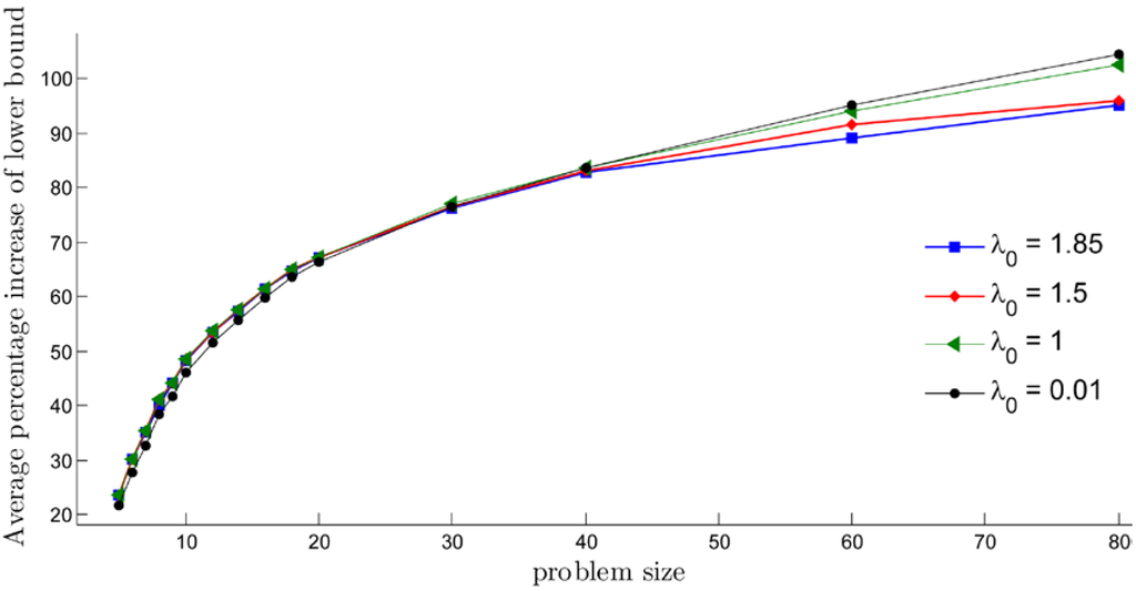
Figure 1. The average percentage increase of the lower bound after applying the modified subgradient optimization method with different ${\lambda }_0$-values.

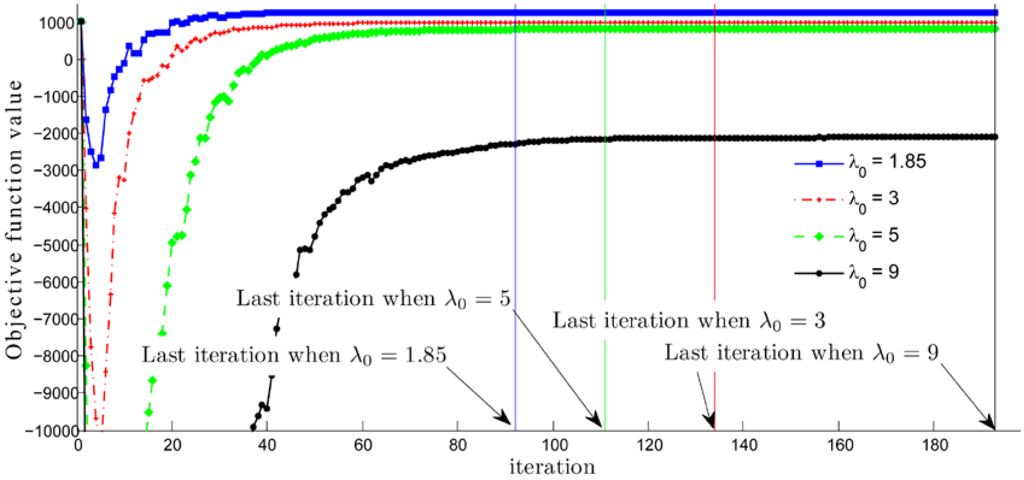
In most practices, authors set the value of the step length constant between 0 and 2, as is discussed in Section 2. However, our computational results have shown that choosing ${\lambda }_0\ge 2$ causes the minimum objective function value of Problem (10), the sink point in Figure 2 and Figure 3, to be deeper in accordance with the bigger ${\lambda }_0$. This value is extremely low, even for a small problem size. This especially occurs for a large problem size and is a major problem. Furthermore, the objective function value at the last iteration is much lower than the value at the earlier iterations, as seen in Figure 2. Consequently, it is not necessary to run the procedure until the stopping criteria is met. Moreover, in terms of lower bound behavior, ${\lambda }_0<2$, in our implementation ${\lambda }_0=1.85$, dominates the other cases with ${\lambda }_0\ge 2$, see Figure 2 and Figure 3. Therefore, it is not necessary to choose ${\lambda }_0$ values greater than 2.

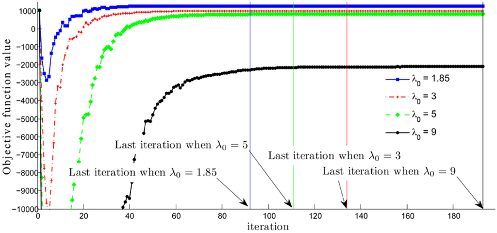
Figure 2. Objective function values, $Z^{*}\left(u^{\left(t\right)}\right)$, at each iteration $t$ , generated by the modified subgradient optimization method for solving an instant of size 8 when ${\lambda }_0\ge 1.85$.

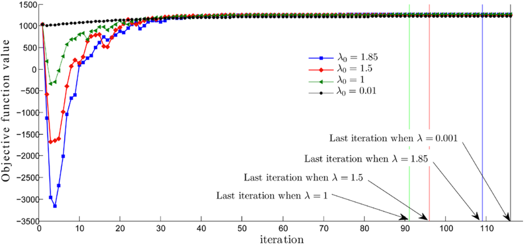
Figure 3. Objective function values, $Z^{*}\left(u^{\left(t\right)}\right)$, at each iteration $t$ , generated by the modified subgradient optimization method for solving an instant of size 8 when ${\lambda }_0\le 1.85$.

Consider the sequence of the objective function values of the considered instants, an example of which can be seen in Figure 3. The values decrease for some early iterations, then quickly increase for some iterations after hitting the possible minimum value (a sink point in the figure). After some iterations (mostly about 30 iterations), the values faintly increase until the stopping criteria are met. However, the objective function values in some iterations may be lower than some previous iterations, but this does not have an effect on the tendency of the sequence, as is shown in Figure 3.

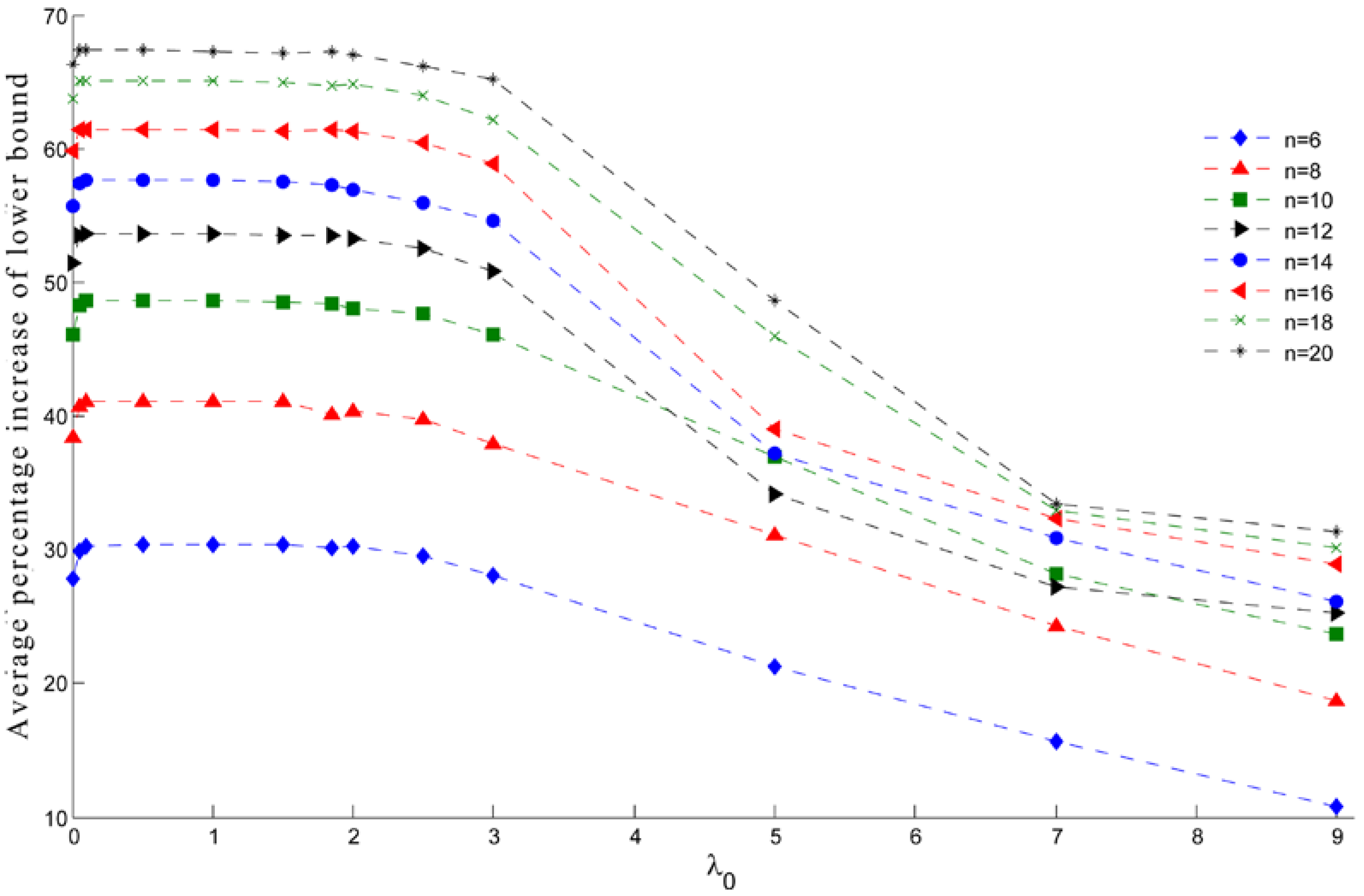
For every instant of problem sizes $n=$ 6, 8, 10, 12, 14, 16, 18, 20, the highest average percentage of increasing of the lower bound occurs when ${\lambda }_0$ lies in between 0.1 and 1, as is shown in Figure 4 and Table 3. These results support the idea of choosing a $\mathsf{\lambda }$-value between 0 and 2. However, the average percentage of increase of the lower bound for the instants of the large problem sizes $n=$ 30, 40, 60, and 80, the highest value occurs when ${\lambda }_0=0.075$ (see Table 3). Furthermore, our computational results have shown that setting ${\lambda }_0$ between 0.05 and 0.1 costs the lowest number of iterations for the procedure (see Table 4).

Figure 4. The average percentage of increase of the lower bound for the P3AP instants of size $n=$ 6, 8, 10, 12, 14, 16, 18, 20 generated by the modified subgradient optimization method with ${\lambda }_0=$ 0.001, 0.001, 0.05, 0.075, 0.1, 0.3, 0.5, 0.75, 1.

Table 3. The average percentage of increase of the lower bound for the P3AP generated by the modified subgradient optimization method with different ${\mathit{\lambda }}_{\mathbf{0}}$-values.

Problem	$\mathsf{\lambda }$
size	0.001	0.01	0.05	0.075	0.1	0.3	0.5	0.75	1
5	19.383	21.886	23.360	23.517	23.388	23.664	23.629	23.677	23.688
6	24.604	27.864	29.917	30.169	30.292	30.348	30.342	30.249	30.347
7	29.387	32.801	35.053	35.311	35.422	35.513	35.490	35.505	35.521
8	34.668	38.362	40.744	40.958	41.054	41.104	41.115	41.091	41.086
9	37.907	41.616	43.939	44.171	44.253	44.263	44.309	44.313	44.288
10	42.018	46.064	48.332	48.497	48.585	48.653	48.642	48.639	48.588
12	47.469	51.489	53.501	53.517	53.668	53.686	53.679	53.682	53.665
14	51.941	55.728	57.421	57.646	57.676	57.667	57.668	57.673	57.632
16	56.453	59.814	61.398	61.394	61.476	61.472	61.472	61.480	61.398
18	60.624	63.762	65.060	65.104	65.101	65.104	65.118	65.089	65.087
20	63.162	66.230	67.383	67.366	67.414	67.420	67.408	67.371	67.265
30	74.366	76.614	77.174	77.197	77.177	77.175	77.166	77.031	76.950
40	81.060	83.725	84.042	84.051	84.043	84.028	83.899	83.818	83.573
60	93.747	95.043	95.160	95.180	95.169	95.133	94.999	94.516	93.945
80	104.453	104.469	104.510	104.525	104.491	104.428	104.174	103.484	102.454

Note: Each bold value shows the highest average percentage of the increase of the lower bound for each problem size

Table 4. The average number of iterations in the modified subgradient optimization method for each problem size with different ${\mathit{\lambda }}_{\mathbf{0}}$-values.

Problem	$\mathsf{\lambda }$
size	0.001	0.01	0.05	0.075	0.1	0.3	0.5	0.75	1	1.25	1.5	1.85
5	349.7	62.2	45.2	40.2	42.0	54.8	48.2	49.8	60.7	54.4	55.8	88.6
6	366.4	80.0	59.4	60.7	60.6	63.1	64.3	68.7	76.5	75.6	73.2	97.2
7	386.0	91.8	69.8	68.9	68.8	75.0	76.0	79.2	90.4	87.3	83.5	105.6
8	380.8	101.1	76.1	75.6	76.1	83.2	87.4	89.2	99.9	96.5	94.2	111.0
9	360.2	108.4	78.3	80.4	80.6	84.3	90.0	95.4	103.2	99.2	96.0	108.0
10	383.5	110.3	80.9	80.0	82.0	90.0	93.6	97.7	107.4	104.2	100.6	110.5
12	371.0	120.0	85.4	86.5	89.5	97.2	98.1	107.2	116.7	113.2	109.2	108.4
14	378.5	127.3	90.2	93.9	97.2	99.8	106.1	115.5	121.3	120.6	115.6	111.4
16	381.5	132.2	93.3	96.5	98.5	104.3	113.2	117.8	130.0	122.5	120.8	111.3
18	364.3	136.0	101.9	100.5	101.0	108.9	115.7	121.4	133.5	131.7	125.8	116.8
20	356.3	141.1	100.9	102.0	103.7	113.5	121.3	125.4	138.1	132.3	126.2	112.1
30	322.2	162.5	111.8	116.5	115.9	125.7	129.7	140.5	152.9	150.1	146.7	114.4
40	296.6	172.8	121.4	124.6	125.2	139.0	144.3	150.7	168.9	163.4	156.7	119.2
60	264.7	204.4	137.2	141.5	139.2	152.7	162.2	172.6	192.6	189.0	184.4	131.1
80	247.8	242.3	154.0	152.2	152.9	170.6	182.8	189.3	249.0	218.0	200.2	148.1

Note: Each bold value shows the lowest average number of iterations.

Since a P3AP is an NP-complete problem [1], each problem has its own properties and it is not easy to find a global solution for this problem. The only known algorithm for finding the global optimal solution for this problem is a branch and bound algorithm. The efficiency of the algorithm depends on the best lower and upper bound found by the algorithm. The subgradient optimization method is one of the methods used for generating a good lower bound for the problem. The method can be applied to the root node or a leaf of the branch and bound tree. Some conditions used in the method may lead to an optimal solution. The exact value for some constants in the method need computer experiments, and the best choice will be made. For our experiments, the variant values of the initial step length constant ${\lambda }_0$, the most suitable are best chosen in the interval [0.1, 1] for small problem sizes, when $n<20$, and [0.05, 0.1] for bigger problem sizes, when $n\ge 20$.

References

- Frieze, A.M. Complexity of a 3-dimensional assignment problem. Eur. J. Op. Res. 1983, 13, 161–164. [Google Scholar] [CrossRef]
- Kumar, S.; Russell, A.; Sundaram, R. Approximating Latin square extensions. Algorithmica 1999, 24, 128–138. [Google Scholar] [CrossRef]
- Gomes, C.; Regis, R.; Shmoys, D. An improved approximation algorithm for the partial Latin square extension problem. Oper. Res. Lett. 2004, 32, 479–484. [Google Scholar] [CrossRef]
- Katz-Rogozhnikov, D.; Sviridenko, M. Planar Three-Index Assignment Problem via Dependent Contention Resolution; IBM Research Report; Thomas, J., Ed.; Watson Research Center: Yorktown Height, New York, NY, USA, 2010. [Google Scholar]
- Magos, D.; Miliotis, P. An algorithm for the planar three-index assignment problem. Eur. J. Op. Res. 1994, 77, 141–153. [Google Scholar] [CrossRef]
- Shor, N. Minimization methods for non-differentiable functions. In Springer Series in Computational Mathematics; Springer-Verlag: Berlin; Heidelberg, Germany, 1985. [Google Scholar]
- Sherali, H.D.; Choi, G. Recovery of primal solutions when using subgradient methods to solve Lagrangian duals of linear programs. Oper. Res. Lett. 1996, 19, 105–113. [Google Scholar] [CrossRef]
- Fumero, F. A modified subgradient algorithm for Lagrangean relaxation. Comput. Op. Res. 2001, 28, 33–52. [Google Scholar] [CrossRef]
- Goffin, J.L. On convergence rate of subgradient optimization methods. Math. Program. 1977, 13, 329–347. [Google Scholar] [CrossRef]
- Held, M.; Wolfe, P.; Crowder, H.P. Validation of subgradient optimization. Math. Program. 1974, 6, 62–88. [Google Scholar] [CrossRef]
- Bazaraa, M.S.; Sherali, H.D. On the choice of step size in subgradient optimization. Eur. J. Op. Res. 1981, 7, 380–388. [Google Scholar] [CrossRef]
- Fischer, M.L. The Lagrangean relaxation method for solving integer programming problems. Manag. Sci. 1981, 72, 1–18. [Google Scholar] [CrossRef]
- Camerini, P.; Fratta, L.; Maffioli, F. On improving relaxation methods by modified gradient techniques. Math. Program. Study 1975, 3, 26–34. [Google Scholar]
- Kim, S.; Koh, S.; Ahn, H. Two-direction subgradient method for non-differentiable optimization problems. Oper. Res. Lett. 1987, 6, 43–46. [Google Scholar] [CrossRef]
- Kim, S.; Koh, S. On Polyak’s improved subgradient method. J. Optim. Theory Appl. 1988, 57, 355–360. [Google Scholar] [CrossRef]
- Norkin, V.N. Method of nondifferentiable function minimization with average of generalized gradients. Kibernetika 1980, 6, 86–89. [Google Scholar]
- Kim, S.; Ahn, H. Convergence of a generalized subgradient method for non-differentiable convex optimization. Math. Program. 1991, 50, 75–80. [Google Scholar] [CrossRef]
- Burkard, R.E.; Froehlich, K. Some remark on 3-dimensinal assignment problems. Methods Op. Res. 1980, 36, 31–36. [Google Scholar]
- Burkard, E. Admissible transformations and assignment problems. Vietnam J. Math. 2007, 35, 373–386. [Google Scholar]
© 2016 by the author; licensee MDPI, Basel, Switzerland. This article is an open access article distributed under the terms and conditions of the Creative Commons by Attribution (CC-BY) license (http://creativecommons.org/licenses/by/4.0/).