
Numerical Simulation of Dense Solid-Liquid Mixing in Stirred Vessel with Improved Dual Axial Impeller


Abstract
:1. Introduction
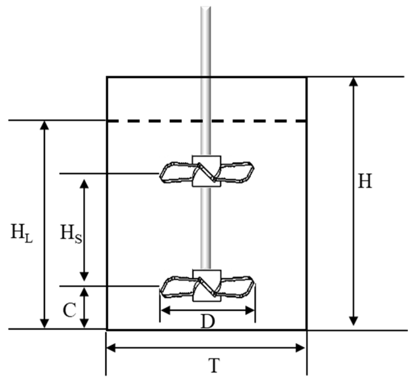
2. System Studied
3. Computational Model and Details
3.1. Equations of Motion
3.2. Turbulence Model
3.3. Interphase Drag Force and Drag Coefficient
3.4. Numerical Details
4. Results and Discussions
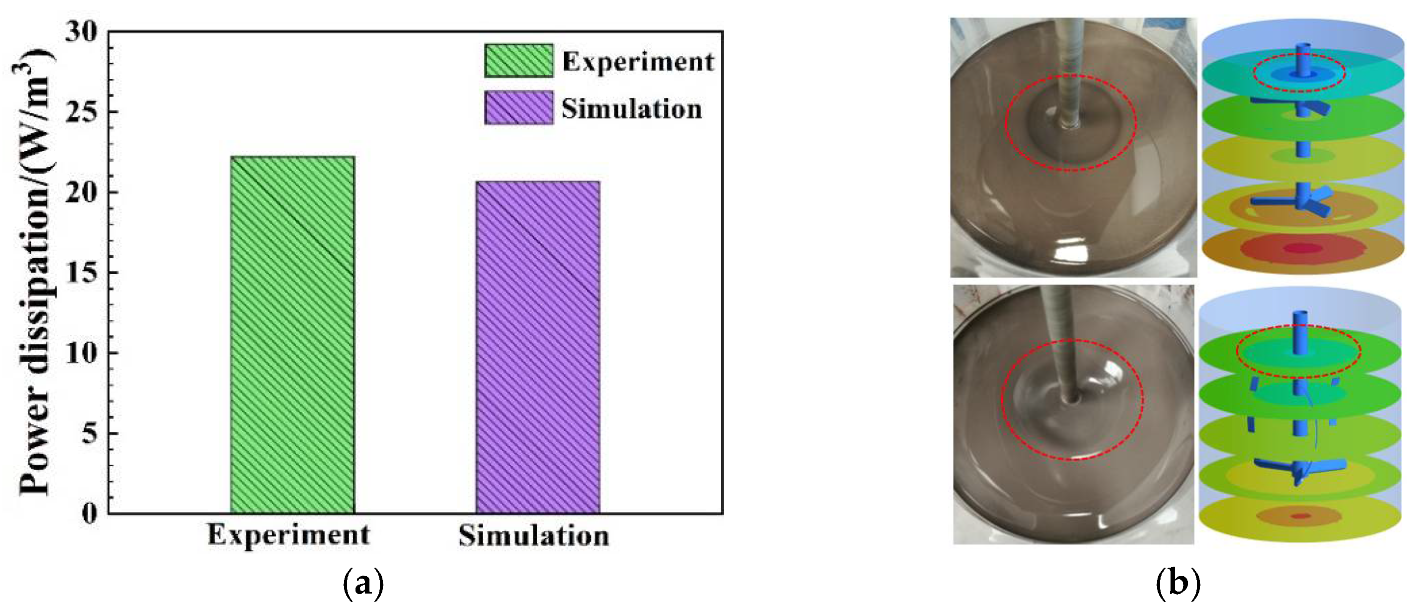
4.1. Verification of Modelling
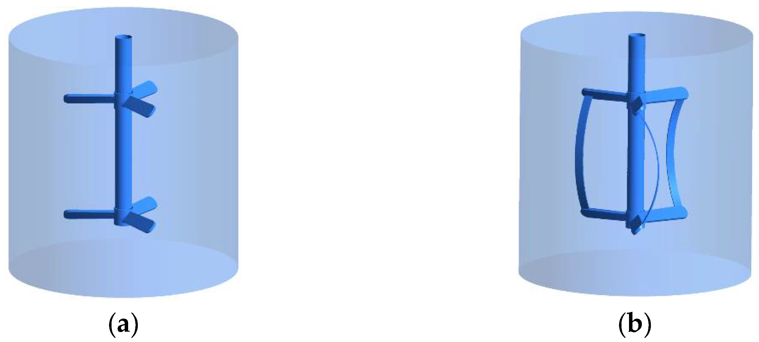
4.2. Strengthening Effects of the Improved Impeller
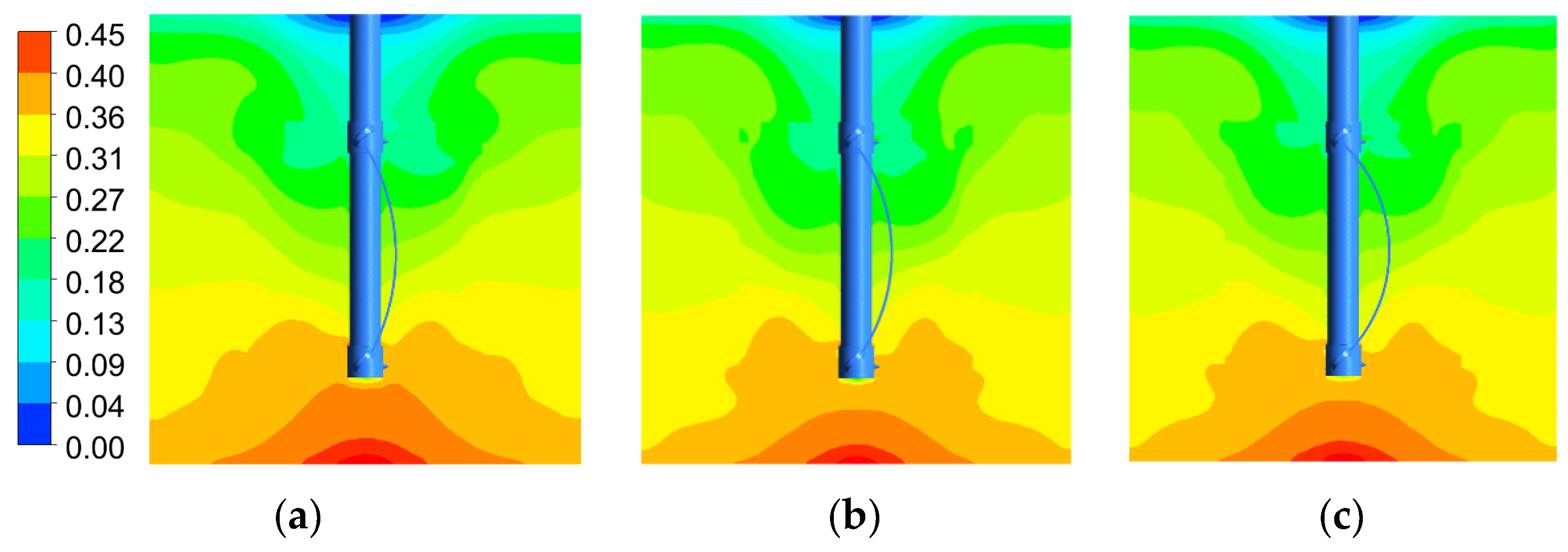
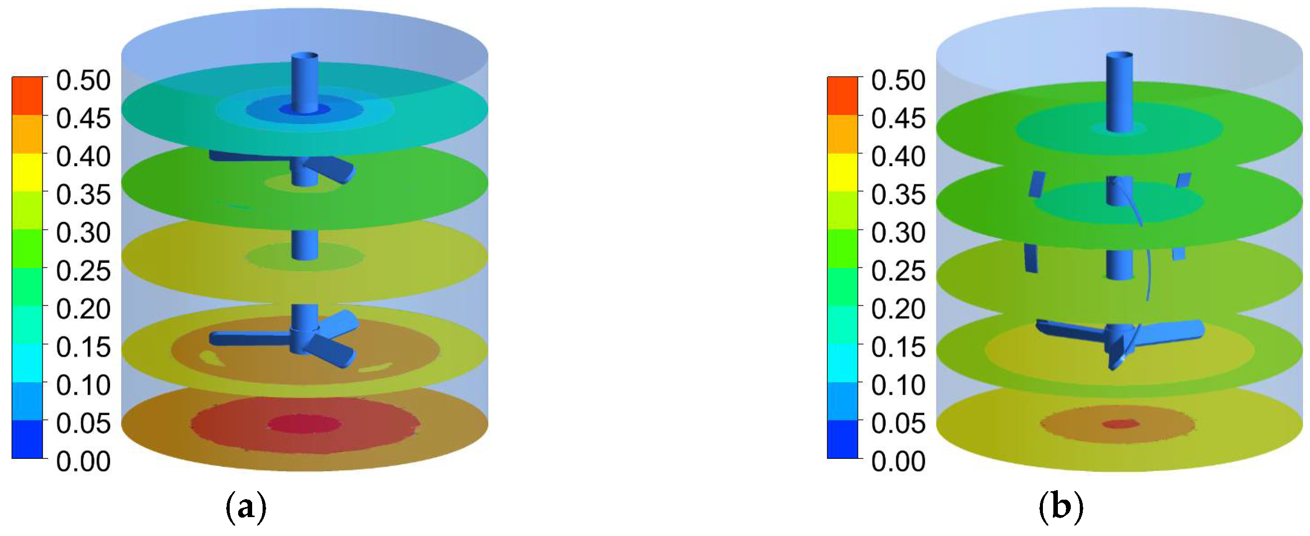
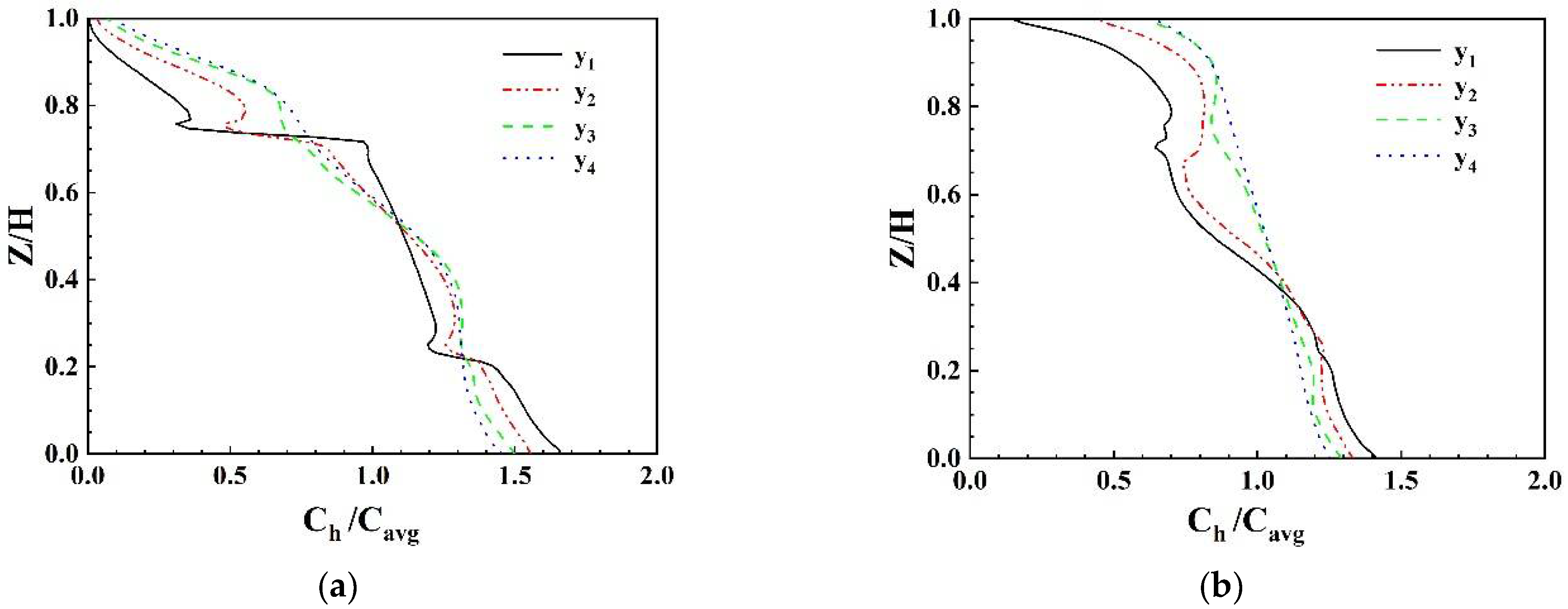
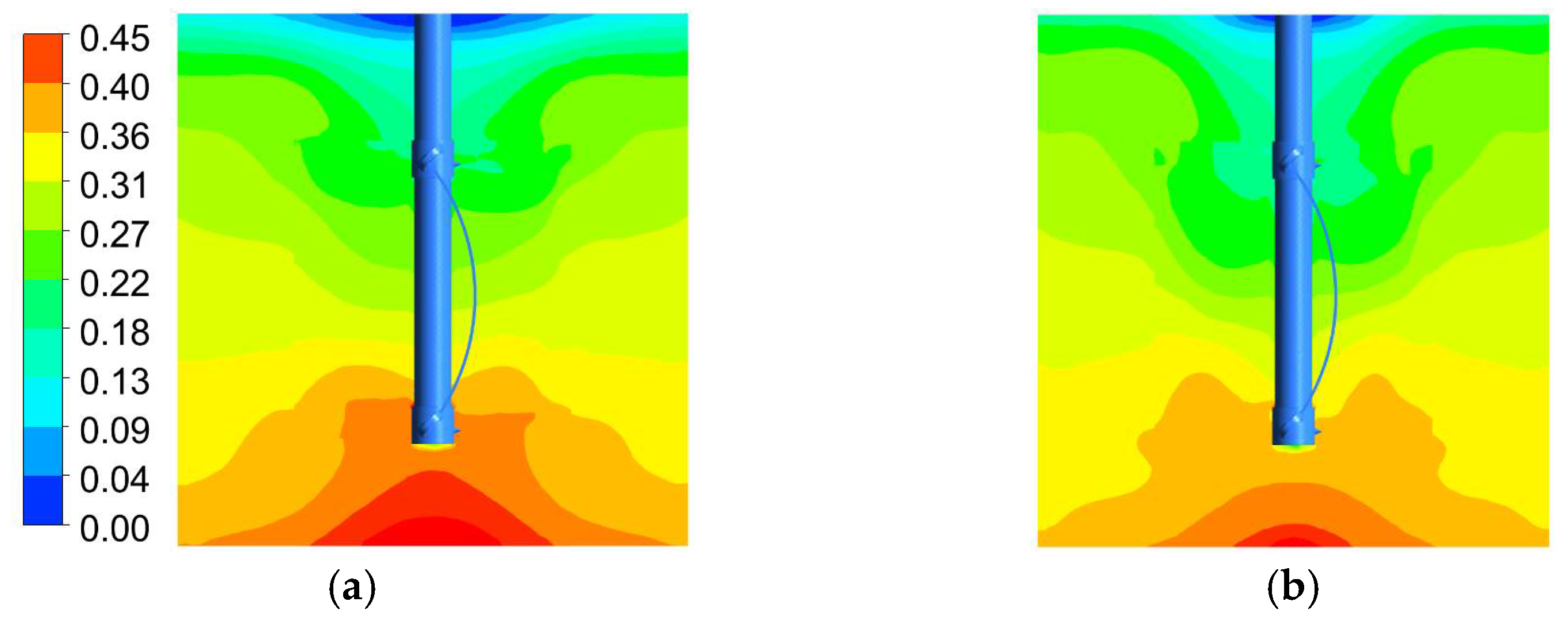
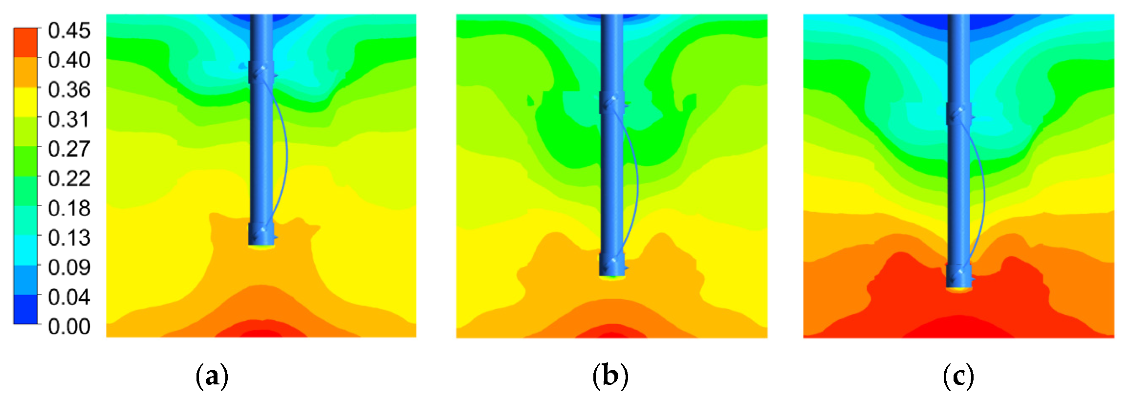
4.2.1. Comparison of Solid Particle Distribution
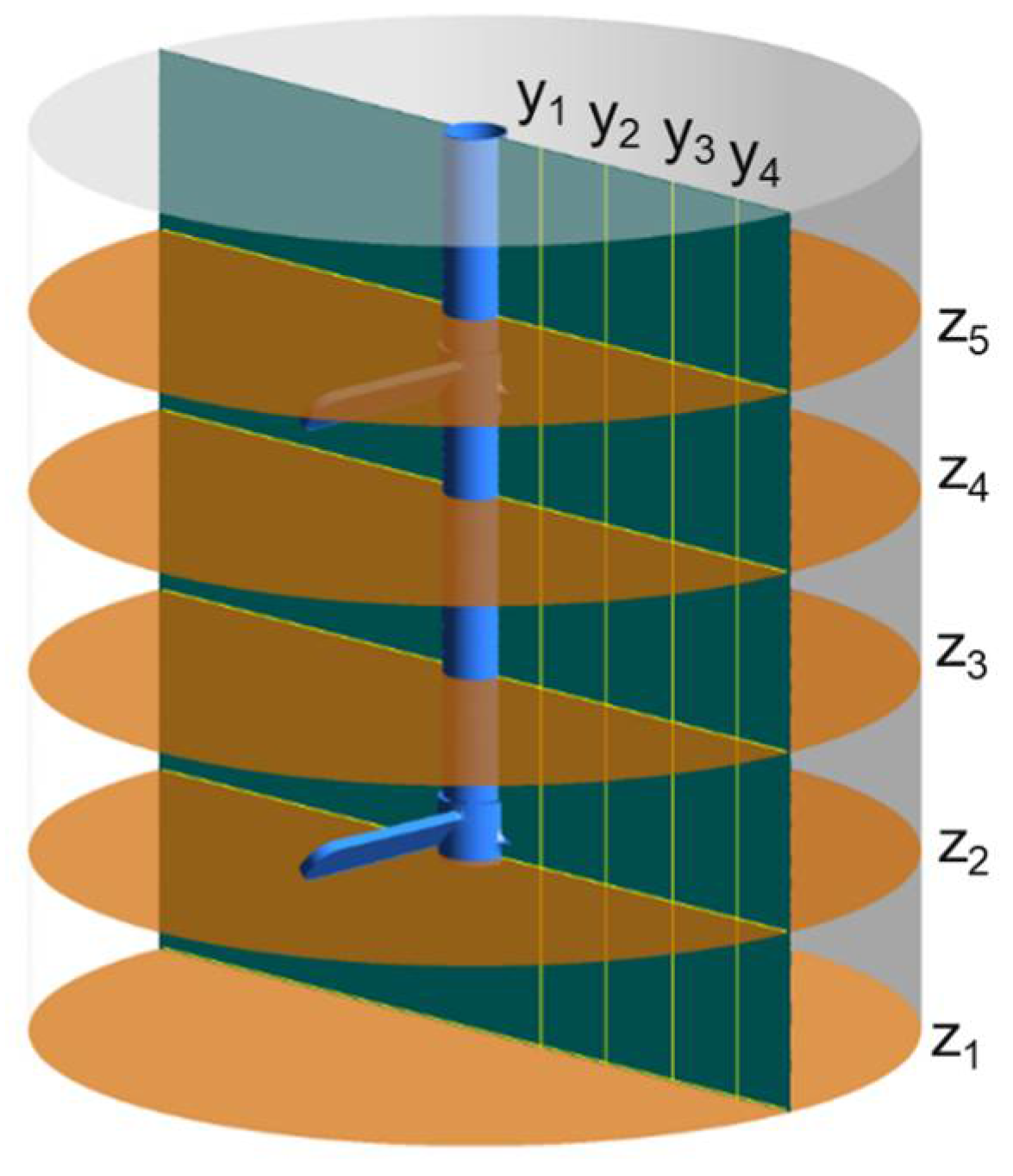
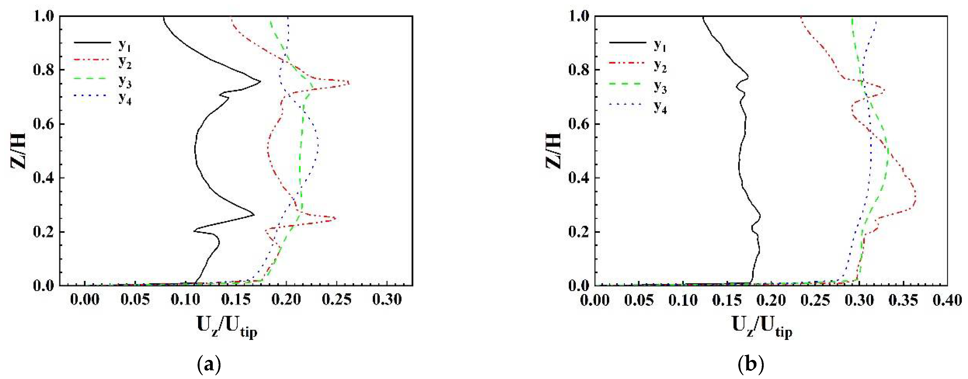
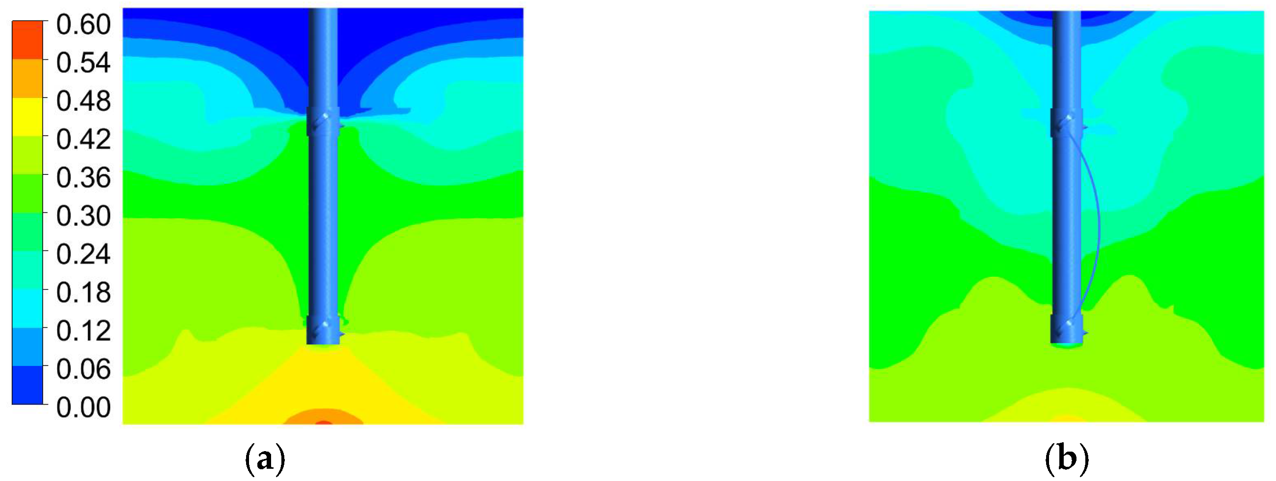
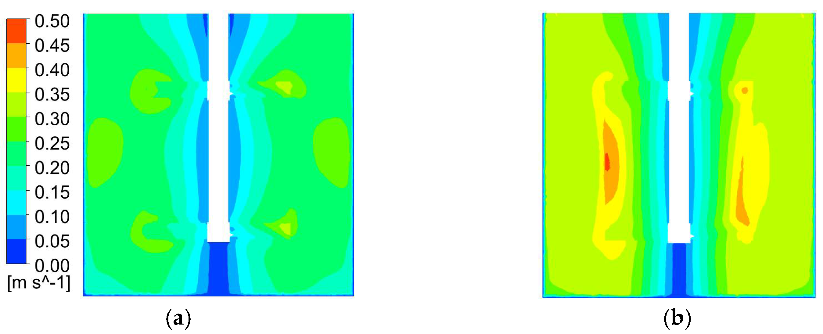
4.2.2. Comparison of Velocity
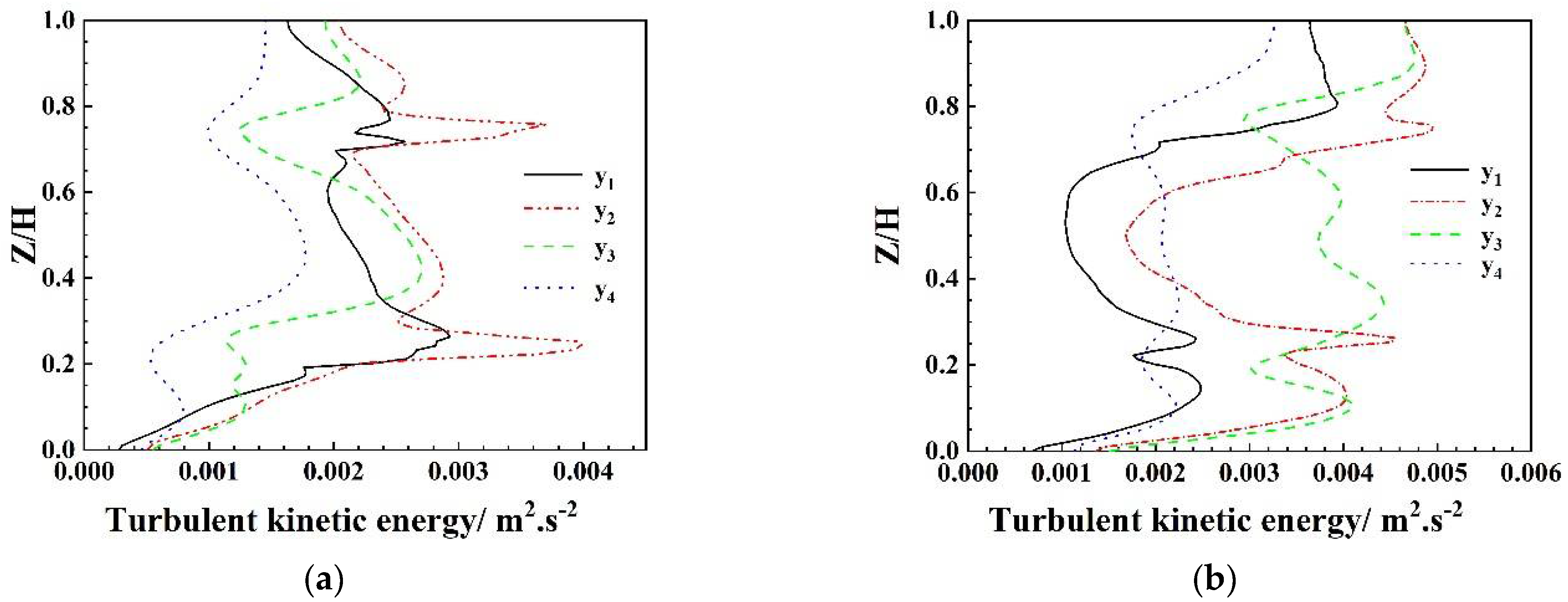
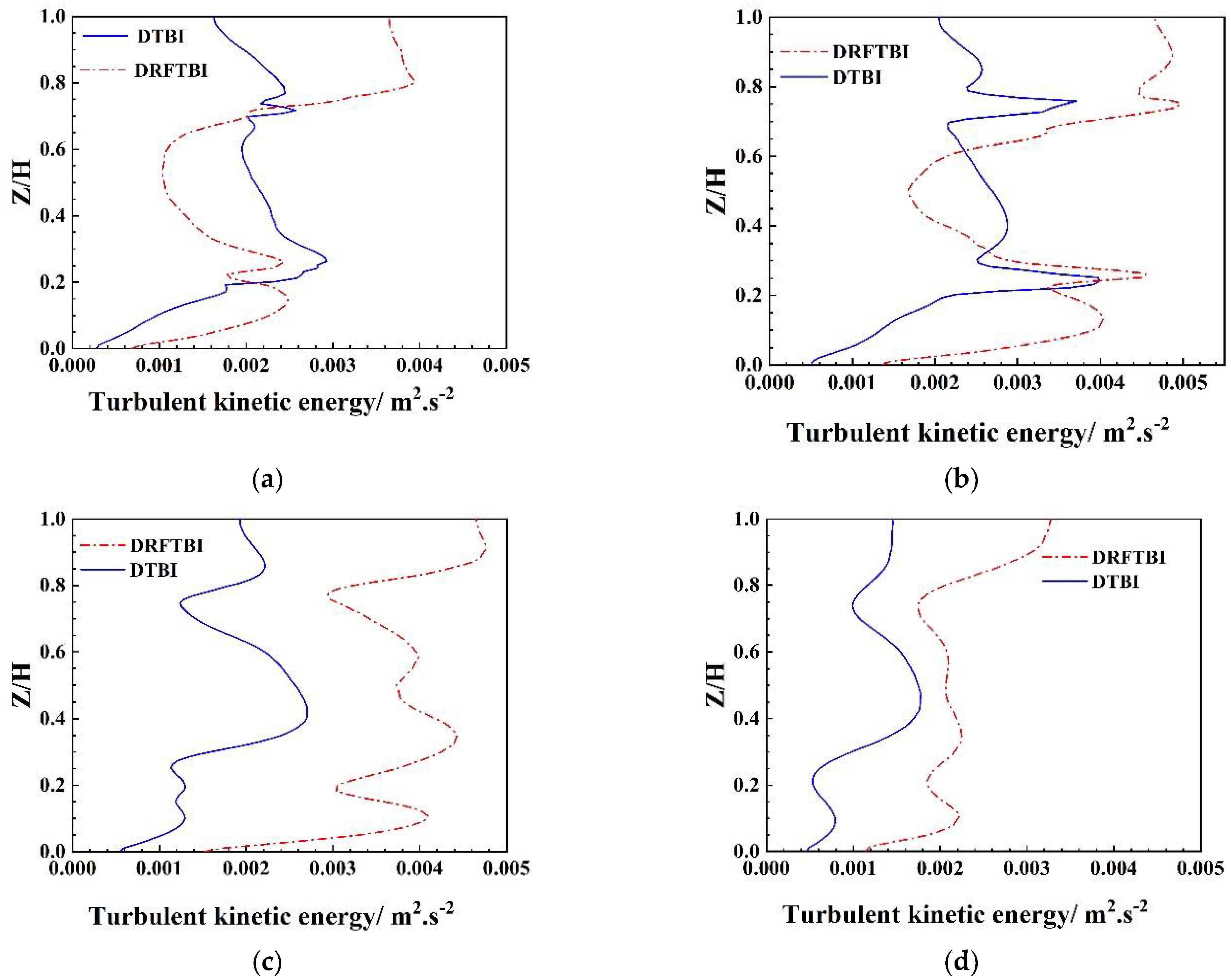
4.2.3. Comparison of Turbulent Kinetic Energy
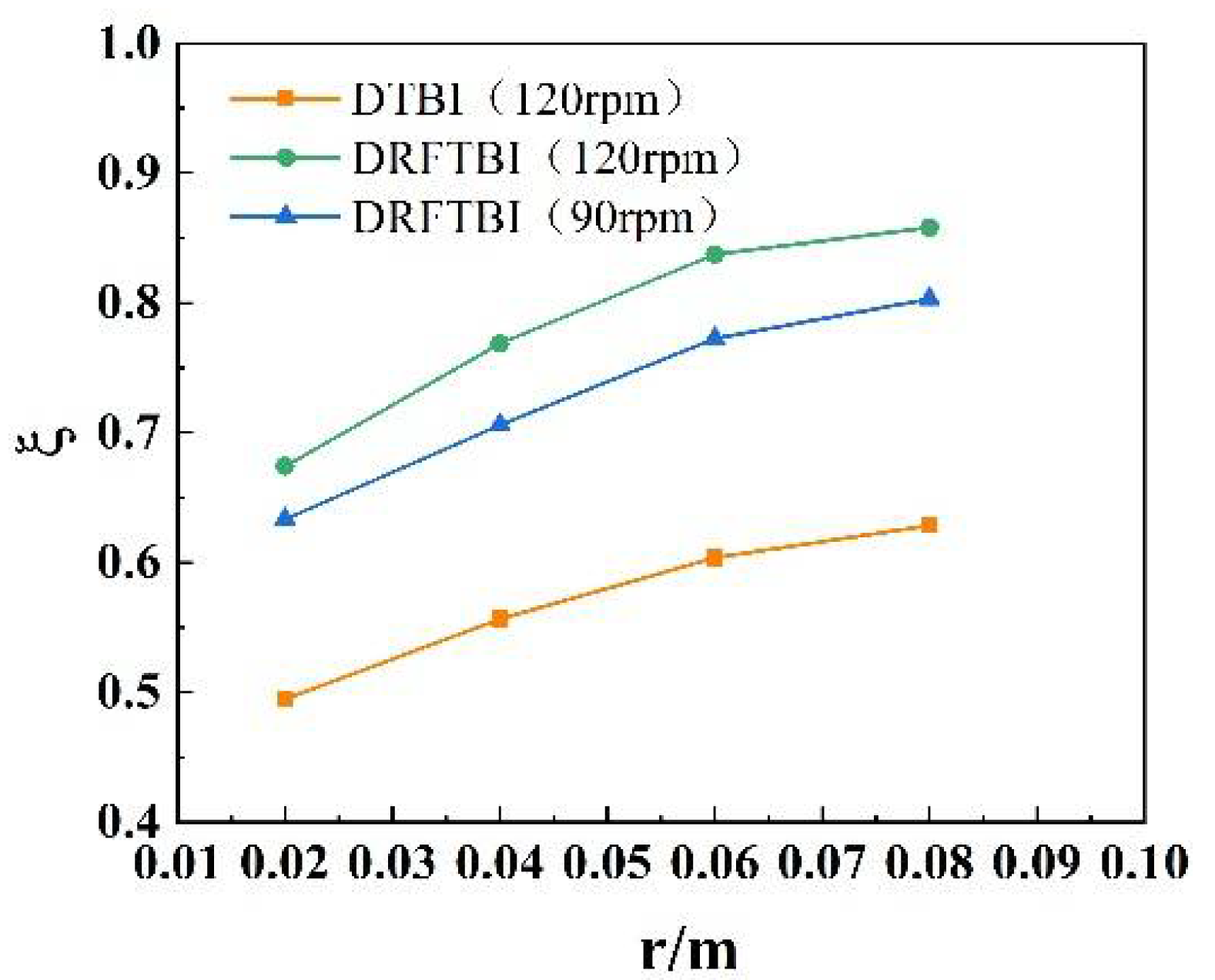
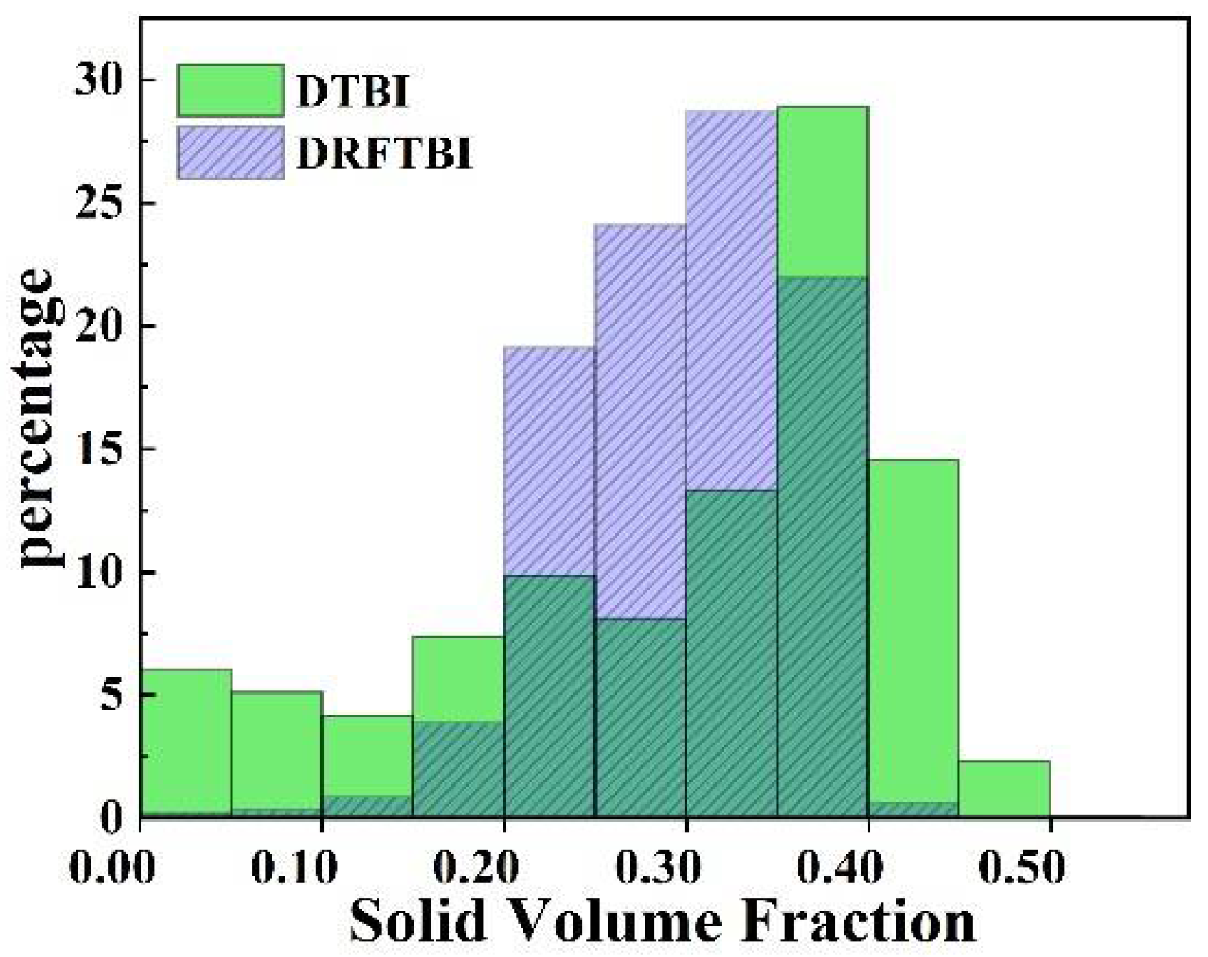
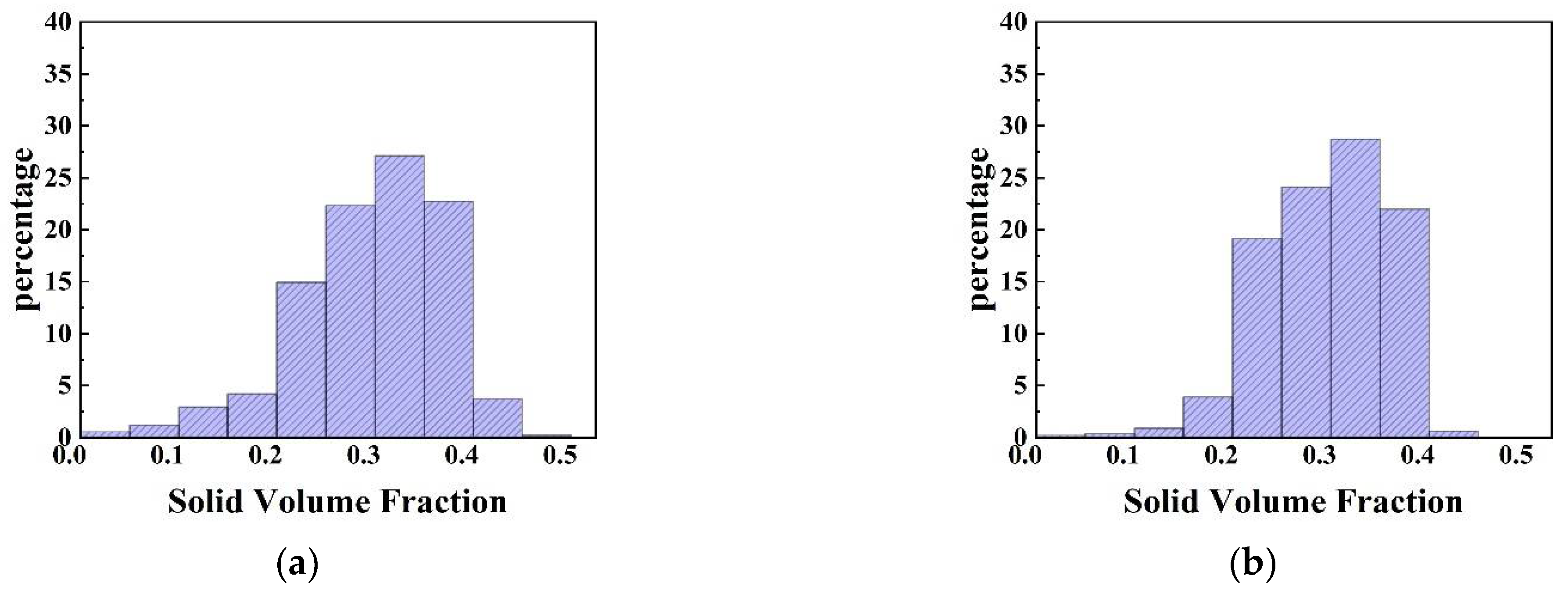
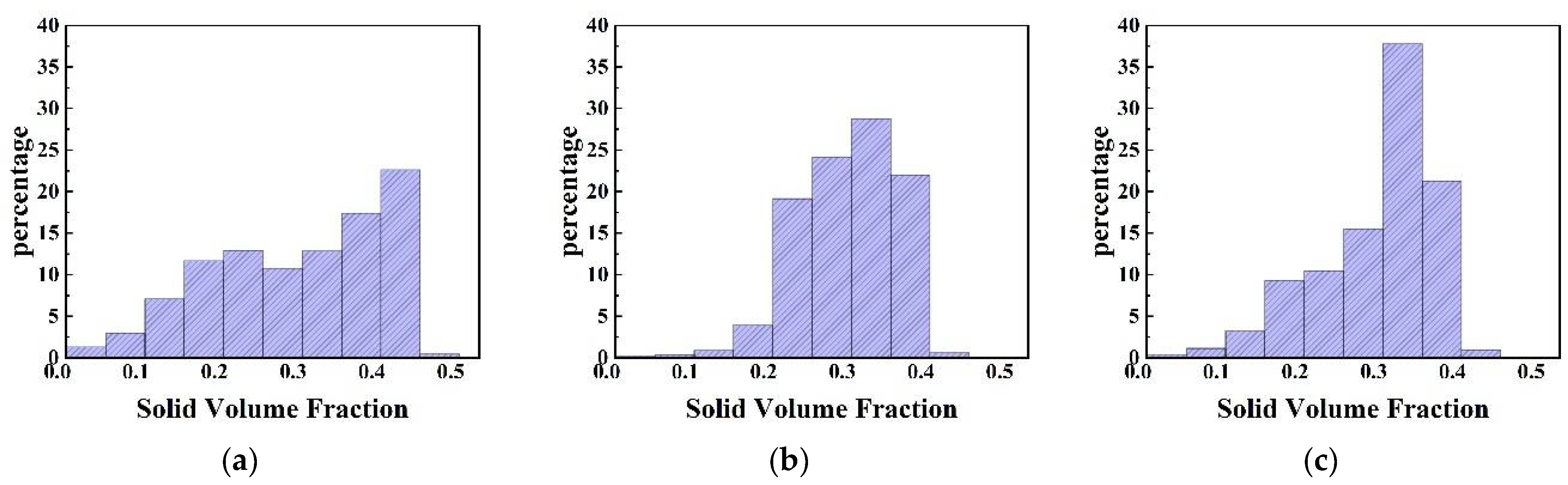
4.2.4. Comparison of Homogeneity
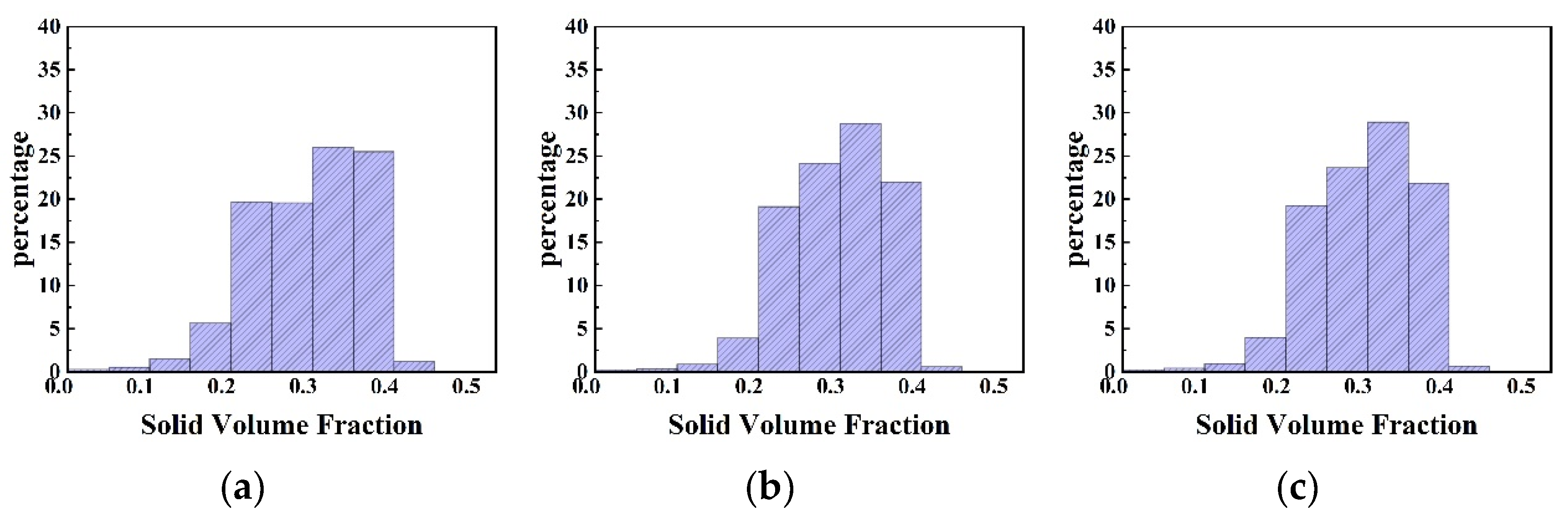
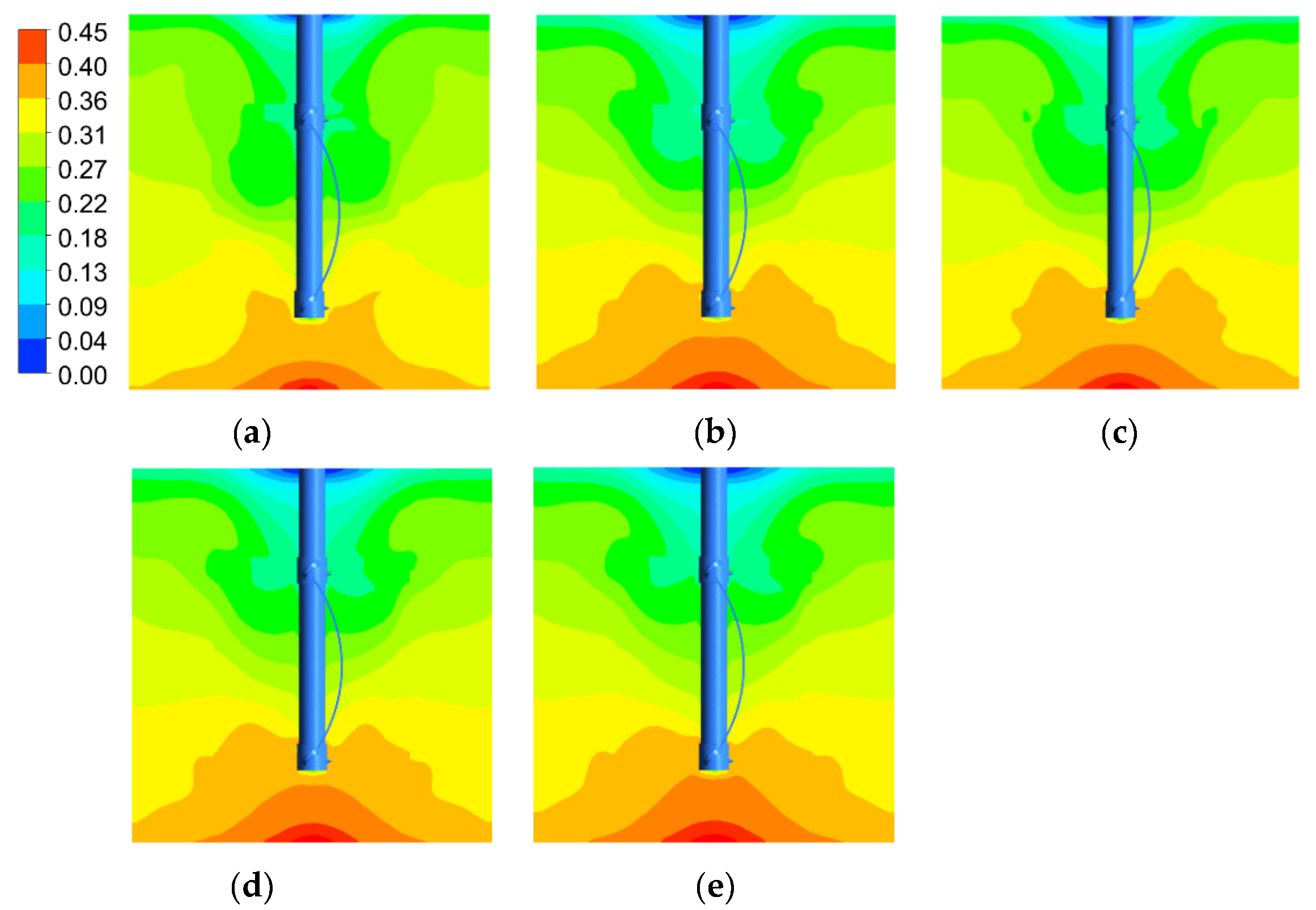
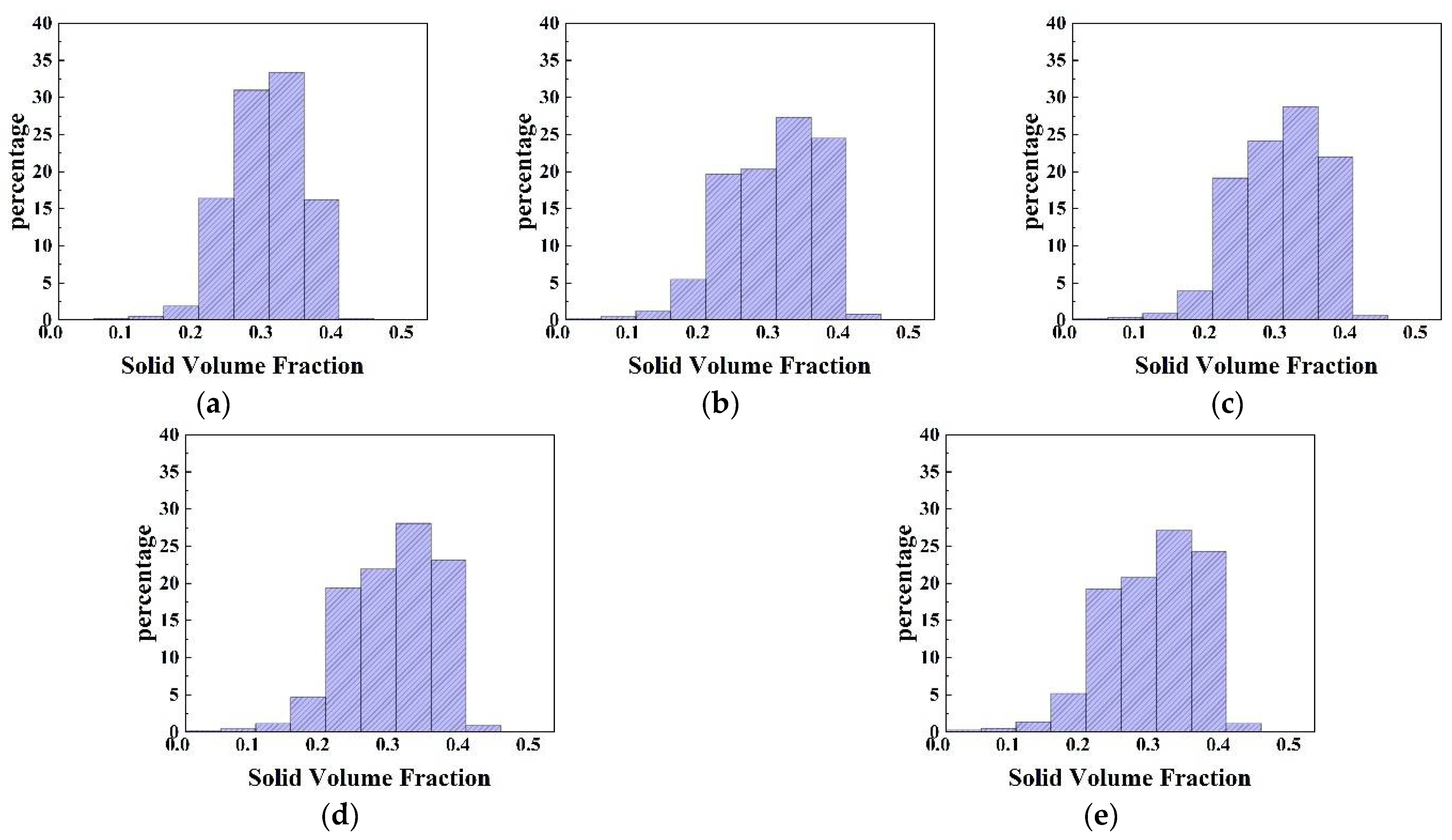
4.3. Effect of Rotation Speed
4.4. Effect of Connection Strap Length
4.5. Effect of Connection Strap Width
4.6. Effect of Off-Bottom Clearance
5. Conclusions
Author Contributions
Funding
Institutional Review Board Statement
Informed Consent Statement
Data Availability Statement
Conflicts of Interest
Nomenclature
| C | off-bottom clearance (m) |
| Ch | local solid volume fraction at height of h |
| Cavg | average solid volume fraction |
| Cε1, Cε2, Cε3, Cμ | ὺparameters in the standard k-ε model |
| CD | drag coefficient |
| D | impeller diameter (m) |
| dp | particle diameter (m) |
| F | interphase momentum transfer term (N) |
| Fdrag | drag force (N) |
| g | gravitational acceleration (m/s2) |
| H | stirred vessel height (m) |
| HL | liquid height (m) |
| HS | interlayer spacing of two impeller (m) |
| k | turbulent kinetic energy (m2/s2) |
| Ma | absolute torque (N.m) |
| Mm | torque measured experimentally (N.m) |
| Mr | residual torque (N.m) |
| N | impeller speed (rpm) |
| n | number of sampling points |
| P | pressure (Pa) |
| Psum | power consumption (W) |
| Pv | specific power consumption (W/m3) |
| r | radial coordinate (m) |
| T | inner diameter of stirred vessel (m) |
| t | time (s) |
| Ui | velocity (m/s) |
| V | total volume of solid and liquid (m3) |
| Greek Letters | |
| ρl | liquid density (kg/m3) |
| ρs | solid density (kg/m3) |
| ρ | density (kg/m3) |
| α | volume fraction |
| αl | liquid phase volume fraction |
| αs | solid phase volume fraction |
| ε | turbulent energy dissipation rate |
| μ | viscosity (Pa·s) |
| μl | liquid phase viscosity (Pa·s) |
| μt | turbulent viscosity (Pa·s) |
| μtl | liquid phase turbulent viscosity (Pa·s) |
| σk , σε | k and ε turbulent Prandtl number |
| ξ | homogeneity |
References
- Carletti, C.; Montante, G.; Westerlund, T.; Paglianti, A. Analysis of solid concentration distribution in dense solid–liquid stirred tanks by electrical resistance tomography. Chem. Eng. Sci. 2014, 119, 53–64. [Google Scholar] [CrossRef]
- Drewer, G.R.; Ahmed, N.; Jameson, G.J. Suspension of High Concentration Solids in Mechanically Stirred Vessels. In Institution of Chemical Engineers Symposium Series; Hemisphere Publishing Corporation: London, UK, 1994; Volume 136, p. 41. [Google Scholar]
- Tamburini, A.; Cipollina, A.; Micale, G.; Brucato, A.; Ciofalo, M. CFD simulations of dense solid–liquid suspensions in baffled stirred tanks: Prediction of solid particle distribution. Chem. Eng. J. 2013, 223, 875–890. [Google Scholar] [CrossRef]
- Woziwodzki, S.; Jędrzejczak, A. Effect of eccentricity on laminar mixing in vessel stirred by double turbine impellers. Chem. Eng. Res. Des. 2011, 89, 2268–2278. [Google Scholar] [CrossRef]
- Zhang, M.; Hu, Y.; Wang, W.; Shao, T.; Cheng, Y. Intensification of viscous fluid mixing in eccentric stirred tank systems. Chem. Eng. Processing Process Intensif. 2013, 66, 36–43. [Google Scholar] [CrossRef]
- Nomura, T.; Uchida, T.; Takahashi, K. Enhancement of Mixing by Unsteady Agitation of an Impeller in an Agitated Vessel. J. Chem. Eng. Jpn. 1997, 30, 875–879. [Google Scholar] [CrossRef] [Green Version]
- Lin, R.; Stuckman, M.; Howard, B.H.; Bank, T.L.; Roth, E.A.; Macala, M.K.; Lopano, C.; Soong, Y.; Granite, E.J. Application of sequential extraction and hydrothermal treatment for characterization and enrichment of rare earth elements from coal fly ash. Fuel 2018, 232, 124–133. [Google Scholar] [CrossRef]
- Zhao, H.L.; Zhang, Z.M.; Zhang, T.A.; Yan, L.I.U.; Gu, S.Q.; Zhang, C. Experimental and CFD studies of solid-liquid slurry tank stirred with an improved Intermig impeller. Oral Oncol. 2014, 50, 2650–2659. [Google Scholar] [CrossRef]
- Gu, D.; Liu, Z.; Xie, Z.; Li, J.; Tao, C.; Wang, Y. Numerical simulation of solid-liquid suspension in a stirred tank with a dual punched rigid-flexible impeller. Adv. Powder Technol. 2017, 28, 2723–2734. [Google Scholar] [CrossRef]
- Gu, D.; Liu, Z.; Qiu, F.; Li, J.; Tao, C.; Wang, Y. Design of impeller blades for efficient homogeneity of solid-liquid suspension in a stirred tank reactor. Adv. Powder Technol. 2017, 28, 2514–2523. [Google Scholar] [CrossRef]
- Li, G.; Gao, Z.; Li, Z.; Wang, J.; Derksen, J.J. Particle-resolved PIV experiments of solid-liquid mixing in a turbulent stirred tank. AIChE J. 2018, 64, 389–402. [Google Scholar] [CrossRef] [Green Version]
- Kohnen, C.; Bohnet, M. Measurement and Simulation of Fluid Flow in Agitated Solid/Liquid Suspensions. Chem. Eng. Technol. 2001, 24, 639–643. [Google Scholar] [CrossRef]
- Guha, D.; Ramachandran, P.A.; Dudukovic, M.P. Flow field of suspended solids in a stirred tank reactor by Lagrangian tracking. Chem. Eng. Sci. 2007, 62, 6143–6154. [Google Scholar] [CrossRef]
- Liu, L.; Barigou, M. Numerical modelling of velocity field and phase distribution in dense monodisperse solid–liquid suspensions under different regimes of agitation: CFD and PEPT experiments. Chem. Eng. Sci. 2013, 101, 837–850. [Google Scholar] [CrossRef]
- Wang, H.; Li, X.; Mao, Z.S.; Yang, C. New invasive image velocimetry applicable to dense multiphase flows and its application in solid–liquid suspensions. AIChE J. 2019, 65, e16668. [Google Scholar] [CrossRef]
- Tamburini, A.; Cipollina, A.; Micale, G.; Brucato, A.; Ciofalo, M. CFD simulations of dense solid–liquid suspensions in baffled stirred tanks: Prediction of suspension curves. Chem. Eng. J. 2011, 178, 324–341. [Google Scholar] [CrossRef]
- Tamburini, A.; Cipollina, A.; Micale, G.; Brucato, A.; Ciofalo, M. CFD simulations of dense solid–liquid suspensions in baffled stirred tanks: Prediction of the minimum impeller speed for complete suspension. Chem. Eng. J. 2012, 193, 234–255. [Google Scholar] [CrossRef]
- Li, X.K. Multiphase Flow and Fluidization, Continuum and Kinetic Theory Descriptions; Gidaspow, D., Ed.; Academic Press: New York, NY, USA, 1993; p. 467, Price $60.00; ISBN 0-12-282770-9. J. Non-Newton. Fluid Mech.1994, 55, 207–208. [Google Scholar]
- Klenov, O.P.; Noskov, A.S. Solid dispersion in the slurry reactor with multiple impellers. Chem. Eng. J. 2011, 176, 75–82. [Google Scholar] [CrossRef]
- Hosseini, S.; Patel, D.; Ein-Mozaffari, F.; Mehrvar, M. Study of Solid−Liquid Mixing in Agitated Tanks through Computational Fluid Dynamics Modeling. Ind. Eng. Chem. Res. 2010, 49, 4426–4435. [Google Scholar] [CrossRef]
- Qi, N.; Zhang, H.; Zhang, K.; Xu, G.; Yang, Y. CFD simulation of particle suspension in a stirred tank. Particuology 2013, 11, 317–326. [Google Scholar] [CrossRef]
- Hashemi, N.; Ein-Mozaffari, F.; Upreti, S.R.; Hwang, D.K. Analysis of mixing in an aerated reactor equipped with the coaxial mixer through electrical resistance tomography and response surface method. Chem. Eng. Res. Des. 2016, 109, 734–752. [Google Scholar] [CrossRef]
- Hashemi, N.; Ein-Mozaffari, F.; Upreti, S.R.; Hwang, D.K. Analysis of power consumption and gas holdup distribution for an aerated reactor equipped with a coaxial mixer: Novel correlations for the gas flow number and gassed power. Chem. Eng. Sci. 2016, 151, 25–35. [Google Scholar] [CrossRef]
- Jegatheeswaran, S.; Kazemzadeh, A.; Ein-Mozaffari, F. Enhanced aeration efficiency in non-Newtonian fluids using coaxial mixers: High-solidity ratio central impeller with an anchor. Chem. Eng. J. 2019, 378, 122081. [Google Scholar] [CrossRef]
- Hashemi, N.; Ein-Mozaffari, F.; Upreti, S.R.; Hwang, D.K. Experimental investigation of the bubble behavior in an aerated coaxial mixing vessel through electrical resistance tomography (ERT). Chem. Eng. J. 2016, 289, 402–412. [Google Scholar] [CrossRef]
- Jegatheeswaran, S.; Ein-Mozaffari, F. Investigation of the detrimental effect of the rotational speed on gas holdup in non-Newtonian fluids with Scaba-anchor coaxial mixer: A paradigm shift in gas-liquid mixing. Chem. Eng. J. 2020, 383, 123118. [Google Scholar] [CrossRef]
- Wang, S.; Parthasarathy, R.; Wu, J.; Slatter, P. Optimum Solids Concentration in an Agitated Vessel. Ind. Eng. Chem. Res. 2014, 53, 3959–3973. [Google Scholar] [CrossRef]


Publisher’s Note: MDPI stays neutral with regard to jurisdictional claims in published maps and institutional affiliations. |
© 2022 by the authors. Licensee MDPI, Basel, Switzerland. This article is an open access article distributed under the terms and conditions of the Creative Commons Attribution (CC BY) license (https://creativecommons.org/licenses/by/4.0/).
Share and Cite
Xiong, X.; Liu, Z.; Tao, C.; Wang, Y.; Cheng, F. Numerical Simulation of Dense Solid-Liquid Mixing in Stirred Vessel with Improved Dual Axial Impeller. Separations 2022, 9, 122. https://doi.org/10.3390/separations9050122
Xiong X, Liu Z, Tao C, Wang Y, Cheng F. Numerical Simulation of Dense Solid-Liquid Mixing in Stirred Vessel with Improved Dual Axial Impeller. Separations. 2022; 9(5):122. https://doi.org/10.3390/separations9050122
Chicago/Turabian StyleXiong, Xia, Zuohua Liu, Changyuan Tao, Yundong Wang, and Fangqin Cheng. 2022. "Numerical Simulation of Dense Solid-Liquid Mixing in Stirred Vessel with Improved Dual Axial Impeller" Separations 9, no. 5: 122. https://doi.org/10.3390/separations9050122
APA StyleXiong, X., Liu, Z., Tao, C., Wang, Y., & Cheng, F. (2022). Numerical Simulation of Dense Solid-Liquid Mixing in Stirred Vessel with Improved Dual Axial Impeller. Separations, 9(5), 122. https://doi.org/10.3390/separations9050122