Development and Optimization of a Gas Chromatography–Mass Spectrometry Analytical Method for Detecting Sulfolane and Benzene Toluene, Ethylbenzene, and Xylenes in Water Samples

Abstract

Sulfolane, an organic solvent widely used in the petrochemical industry, has raised concerns due to its potential health risks and environmental mobility. Toxicological studies suggest that it may negatively affect human and ecological health, highlighting the need for risk assessments. Alongside sulfolane, BTEX compounds (benzene, toluene, ethylbenzene, and xylenes) are commonly present in petrochemical operations, and their migration may be influenced by sulfolane. This study developed a gas chromatography–mass spectrometry (GC-MS) method for simultaneous analyses of sulfolane and BTEX in water. The sample preparation was designed for simplicity to allow for easy implementation without specialized equipment. The method was characterized, validated, and its ruggedness was tested through experimental design. The method was then applied to evaluate the stability of water samples under various storage conditions, and to analyze 97 real water samples collected from a contaminated site in Alberta, Canada. The results identified 17 samples with sulfolane concentrations exceeding the maximum limits for aquatic life preservation, and three samples with detectable toluene levels. These findings highlight the need for further research to better understand contamination profiles and assess associated risks.

1. Introduction

Sulfolane (1λ⁶-Thiolane-1,1-dione; Figure 1) is an organic solvent with numerous exceptional properties, including a high boiling point, thermal and chemical stability, and miscibility with both polar and many non-polar solvents [1,2,3]. These attributes have led to its widespread use in various industries, such as petrochemical refining, polymer production, and battery manufacturing [1]. However, the extensive use of sulfolane increases the risk of environmental release, either through accidental spills or improper waste management. Numerous contamination incidents have been reported in countries such as Canada, the United States, and Australia [4]. Once released into the environment, sulfolane readily dissolves in water, and shows minimal adsorption onto soil and rock, enabling it to contaminate groundwater and disperse over large areas [4]. Furthermore, its significant chemical stability necessitates specialized conditions for degradation, which are not typically found in groundwater [5]. Groundwater discharges can subsequently contaminate surface water and natural freshwater reservoirs.

Sulfolane has been identified as a neurotoxin, causing seizures in rodents and monkeys following acute high-dose exposure [6,7]. While accidental exposure to such high doses is uncommon, the primary concern lies in chronic, low-dose exposure. Studies suggest potential health impacts, including reduced white blood cell counts in rats and altered liver biochemical function tests in guinea pigs [8]. Although the relevance of these findings to human health remains uncertain, the combination of sulfolane’s potential toxicity, extensive industrial use, and high environmental mobility and persistence emphasizes the importance of monitoring and risk assessment. The measurement of sulfolane concentrations in water resources is an essential first step in evaluating its environmental and health risks.

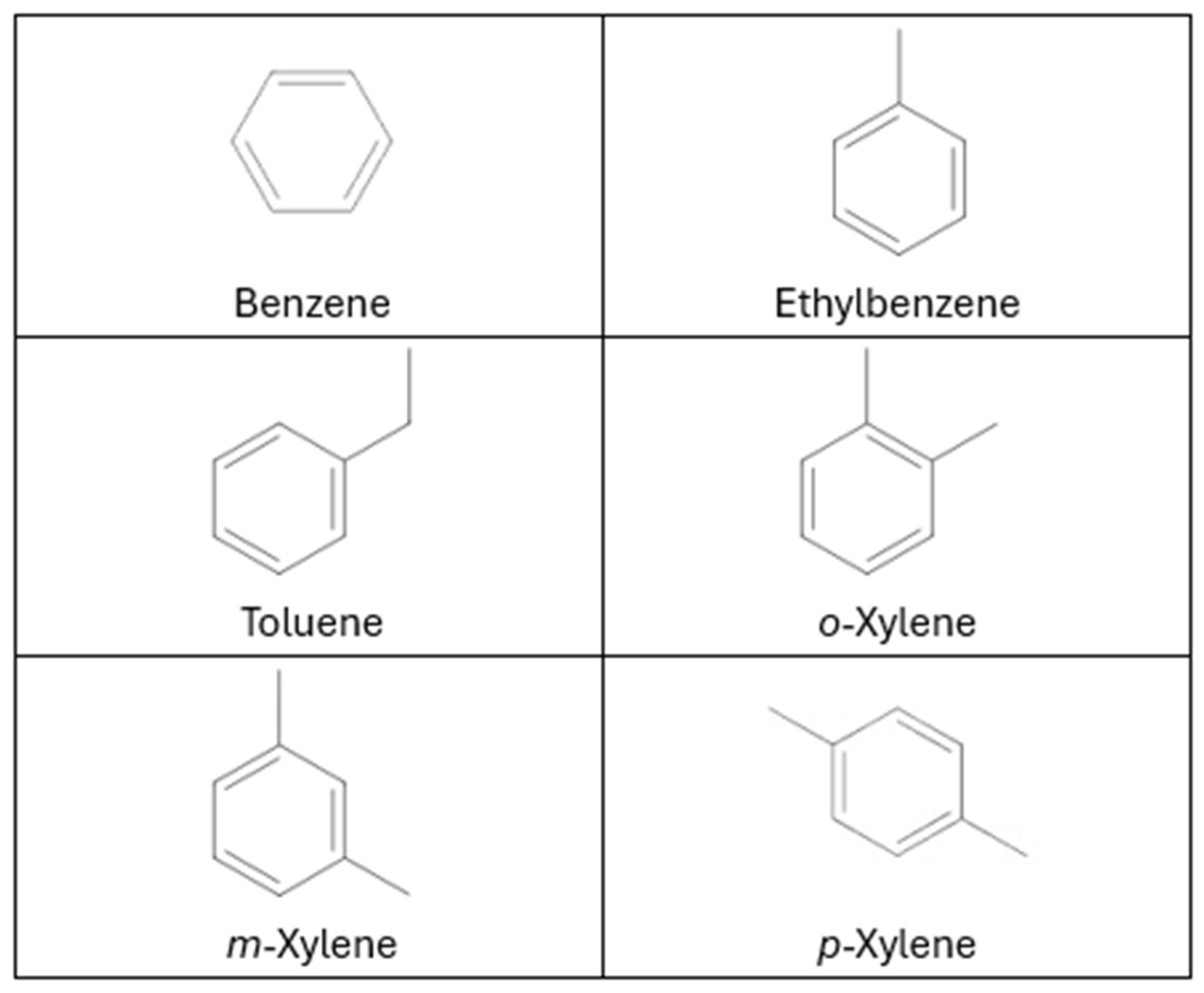
In addition to sulfolane, volatile organic compounds (VOCs) are closely associated with the petrochemical industry. VOCs comprise a diverse group of organic pollutants with varying toxicological profiles [9]. Among these, benzene, toluene, ethylbenzene, and xylenes (Figure 2), collectively known as BTEX, are frequently detected, and serve as representative VOCs due to their widespread occurrence and considerable health effects [9,10,11,12]. BTEX compounds are aromatic hydrocarbons derived from crude oil through refining processes that often involve solvents. Sulfolane is a common solvent used in these processes, making it a potential co-contaminant with BTEX compounds [1]. Additionally, sulfolane may influence the solubility, concentration, and mobility of BTEX in water. Simultaneous analysis of sulfolane and BTEX at contaminated sites can provide critical insights into the interactions between these pollutants and their collective impact on the environment and human health.

Sulfolane is an emerging contaminant that remains largely unregulated worldwide. In Canada, regulatory limits for sulfolane have been established, though significant discrepancies exist among recommended maximum values, primarily due to insufficient toxicity data [13]. Environment Canada specifies maximum sulfolane concentrations of 50 mg/L for freshwater aquatic life, 0.5 mg/L for irrigation, and 0.09 mg/L for groundwater [8]. Similarly, the Government of Alberta adopts these limits for freshwater aquatic life and groundwater, but sets thresholds of 0.8 mg/L for irrigation and 0.09 mg/L for drinking water [14]. In British Columbia, the drinking water limit is also 0.09 mg/L [15]. In contrast, Health Canada recommends a much higher screening value of 0.3 mg/L for drinking water [16].

Unlike sulfolane, maximum contaminant levels (MCLs) for BTEX compounds are well-defined by most regulatory authorities. In Canada, Environment and Climate Change Canada provides long-term guideline concentrations for BTEX to protect aquatic life: 0.59 mg/L for benzene, 0.03 mg/L for toluene, and 0.07 mg/L for both ethylbenzene and xylenes [17]. Health Canada’s maximum acceptable concentrations (MACs) for drinking water are 0.005 mg/L for benzene, 0.06 mg/L for toluene, 0.14 mg/L for ethylbenzene, and 0.09 mg/L for xylenes [18]. The availability of clear regulatory limits for BTEX facilitates the interpretation of environmental monitoring results and risk assessments for these compounds.

Both sulfolane and BTEX are commonly analyzed using gas chromatography–mass spectrometry (GC-MS) due to their sufficient volatility for GC [19,20,21]. The incorporation of MS enhances the selectivity of the method, which is crucial, given the potential presence of interfering co-contaminants. However, the primary distinction between their analyses lies in the sample preparation techniques.

For sulfolane analyses in water samples, two official methods have been established, both of which rely on very large volumes of chlorinated solvents [20,21]. Additionally, various alternative methods have been reported in the literature, most of which employ dichloromethane (DCM) or toluene for sulfolane extraction prior to GC-MS analysis [22,23,24,25,26]. These techniques often involve complex sample preparation procedures.

In contrast, BTEX analysis typically requires preconcentration using solvent-free extraction techniques, such as purge-and-trap [19,27,28]. While these methods enhance sensitivity, they also demand specialized instrumentation and involve elaborate sample preparation. Moreover, purge-and-trap is not suitable for sulfolane analysis, as sulfolane exhibits low volatility and does not partition into the headspace in significant amounts.

In this study, we developed a GC-MS method for the simultaneous quantification of sulfolane and BTEX in water samples with very simple sample preparation. While numerous studies have focused on these compounds individually, to the best of our knowledge, no existing research has examined both sulfolane and BTEX simultaneously in water. The objective of this study was to establish a simple and straightforward GC-MS-based analytical approach with minimal organic solvent use, enabling efficient detection of both compound classes. An additional goal was for the method to utilize the same instrumental configuration used for sulfolane and BTEX analysis in methanolic rock extracts, described in a separate contribution, allowing both rock and water samples to be analyzed without changing the instrument configuration [29].

2. Materials and Methods

2.1. Chemicals and Reagents

Analytical-grade sulfolane (purity: ≥99.8%) was obtained from MilliporeSigma Canada Ltd. (Oakville, ON, Canada), and used for the preparation of calibration standards and spiking samples. A certified sulfolane residual solvent standard was sourced from Restek Corporation (Bellefonte, PA, USA) for the preparation of quality control (QC) samples. Analytical standards of benzene, toluene, ethylbenzene, and xylene (BTEX) and a high-concentration BTEX certified reference material were also procured from MilliporeSigma Canada Ltd., and employed in the preparation of calibration standards and QC samples, respectively. Sulfolane-d8, used as a surrogate standard for sulfolane, was supplied by Toronto Research Chemicals (Toronto, ON, Canada). Toluene-d8, used as a surrogate standard for BTEX, was obtained from Cambridge Isotope Laboratories, Inc. (Tewksbury, MA, USA). DCM (SupraSolv^® grade for GC-MS) was purchased from MilliporeSigma Canada Ltd., and used for extraction and standard preparation. Blank samples were prepared using tap water.

2.2. Sample Collection

A total of 97 surface and shallow groundwater samples, including 47 duplicates, were collected in June 2024 from a former industrial site in central Alberta, Canada. Surface water samples were obtained from a first-order stream at the contaminated site. The samples were collected with a peristaltic pump in pre-cleaned 40 mL glass vials, filled to the brim to minimize the loss of volatile compounds, and sealed with airtight caps. To produce duplicate samples, two vials were filled alternately. The downside of this approach was that the vials remained open to the atmosphere for a longer time, potentially increasing losses of volatile compounds. However, this was deemed an acceptable compromise. In the case of groundwater collection, the procedure was similar, except that in some cases, the amount of groundwater that could be drawn at one time was insufficient to fill the vials, and the collection had to be resumed at a different time. Samples collected in this way cannot be treated as true duplicates.

All samples were transported to the laboratory at the University of Waterloo in an insulated cooler within 48 h of collection and were refrigerated upon arrival. Sample processing and analysis were completed within 72 h of arrival, ensuring a total holding time of less than five days.

2.3. Sample Preparation

To simplify the sample preparation procedure, an in-vial extraction method was employed. For the extraction of sulfolane and BTEX from water samples, 0.500 mL of DCM containing 400 µg/L of sulfolane-d8 and toluene-d8 as surrogate standards was added to a GC vial. Subsequently, 1.00 mL of the water sample was dispensed into the vial using an automatic pipette. The vial was sealed and vortex-shaken for 30 s to ensure thorough extraction and partitioning of analytes into the DCM phase. Samples prepared in this way were then loaded onto the instrument’s autosampler tray for injection and analysis.

2.4. Gas Chromatography–Mass Spectrometry Analysis

A GC-MS method for the analysis of sulfolane and BTEX was developed using an Agilent 6890 GC coupled with a 5973N MS detector (Agilent Technologies, Wilmington, NC, USA). In this analytical approach, the target compounds are initially separated on a GC column based on their volatility. The separated analytes are then introduced into the mass spectrometer, where they are ionized and further distinguished according to their mass-to-charge (m/z) ratios. Owing to the distinctive ionization patterns of individual compounds, MS detection offers significantly enhanced selectivity compared to other GC detectors. The parameters of the method developed are summarized in Table S1.

2.5. Method Validation and Characterization

The method was validated in accordance with the EPA Method Validation Guidelines for Chemical Methods of Analysis [30]. In summary, the linearity of the response was evaluated across a range of 10 µg/L to 8000 µg/L for all compounds. Initial assessments were performed through visual inspection, followed by confirmation using a lack-of-fit F-test. Precision and accuracy were characterized by preparing a set of samples consisting of 10 blank water matrices spiked at two different concentrations. These spiked samples were analyzed, bracketed by two sets of calibration standards, with the procedure repeated three times over three separate days. Data from these analyses were processed to validate and characterize the method’s performance.

Selectivity was demonstrated by employing MS detection and confirming the absence of interferences in spiked samples. Method bias and trueness were assessed through the average recovery of spiked samples, which fell within an acceptable range of 70% to 120%. Precision was quantified by calculating the relative standard deviation (RSD) of the spiked samples, with all compounds exhibiting RSD values below 20%. The limits of detection (LOD) and quantification (LOQ) were determined as three times and ten times the standard deviation (SD) of the lowest concentration spiked samples, respectively. It is important to note that the spiked concentration did not exceed three times the calculated LOQ.

2.6. Method Ruggedness Testing

To assess the ruggedness of the analytical method, a Plackett–Burman experimental design with 11 factors was developed using Minitab^® (ver. 2.21, Minitab, LLC, State College, PA, USA). The study included several factors: the presence or absence of vortex-shaking, reinjection from a pierced vial, a 24 h delay before injection, sample temperature during preparation, needle washing with methanol only, and the use of 0.45 mL of DCM for extraction. The experimental results were subsequently imported into the software, and analysis of variance (ANOVA) was conducted to interpret the findings.

2.7. Sample Hold Time and Analytes’ Stability

To assess the stability of the water samples, two sets were prepared and stored under different conditions. The first set was stored at room temperature (21–25 °C) on a laboratory bench throughout the duration of the study. The second set was refrigerated at 4 °C. Both sets of samples were analyzed at designated intervals, extending up to 23 days.

2.8. Analysis of Water Samples

The water samples collected were analyzed using the validated method. For samples with replicates, analyses were performed on different days to evaluate the method’s robustness and the reproducibility of results. Prior to each analysis, the MS was tuned. Sample analyses were bracketed by calibration standards, with a total of 12 QC samples injected at regular intervals to ensure result validity. Reagent blanks were injected before and after the calibration standards and once every 10 samples to check for injector carryover. Any results below the LOD were disregarded, while results between the LOD and the LOQ were considered positive detections.

3. Results and Discussion

3.1. Sample Preparation Method

The sample preparation method was designed with a focus on simplicity, aiming to minimize the number of steps involved. The most straightforward approach would be direct aqueous injection into the GC, eliminating sample preparation entirely. This technique has been successfully employed in a few studies for sulfolane analysis. However, it requires an on-column injection system, which presents several challenges. Firstly, on-column injectors are less commonly available compared to split/splitless injectors. Secondly, direct injection of water samples, particularly those from contaminated sites, can introduce a high level of matrix contaminants, leading to increased maintenance requirements for the GC system. For these reasons, a split/splitless injector was selected due to its widespread availability and robustness.

With split/splitless injection, direct aqueous injection is not feasible. Water’s high vapor expansion significantly limits the injection volume, reducing sensitivity. Additionally, the MS detector is not well-suited for direct water injections, as water can disrupt the vacuum inside the mass analyzer and interfere with ionization. To address these limitations, an extraction step was incorporated to transfer the target analytes into an organic solvent prior to GC-MS analysis. To further simplify the process, the extraction was designed to take place directly within the GC vials, eliminating the need for phase separation before analysis. This approach minimizes the risk of analyte loss, particularly for volatile compounds such as BTEX.

While a non-chlorinated solvent would have been preferable to mitigate environmental concerns, DCM was selected due to its high density, which allows it to form a distinct layer beneath the aqueous phase. This property enabled automated sampling directly from the DCM layer without the need for an additional transfer step, reducing sample handling, duplicate vials requiring disposal or cleaning, and potential losses. Although autoinjectors can be set up to aspirate only from the upper layer of a vial if a solvent less dense than water is used, this setup requires precise adjustments. Even minor variations in vial dimensions could lead to unintended water aspiration, which would introduce excessive vapor volume into the GC inlet, causing contamination and requiring extensive cleaning. Additionally, the water layer above the DCM phase acts as a barrier, reducing solvent evaporation and potentially enhancing sample stability while stored on the autosampler tray before the injection.

To expedite analyte partitioning into the organic phase, a vortex-shaking step was incorporated into the sample preparation method. While the results in Section 3.4 indicate that vortex-shaking had minimal impact on the quantified analyte concentrations when surrogate standards were used, it did influence analyte response, thereby improving the overall sensitivity of the analytical method.

3.2. GC-MS Method of Analysis

As discussed in Section 3.1, the split/splitless injection system was selected due to its greater availability and reduced maintenance requirements. While splitless injection would have been preferable for maximizing sensitivity, it resulted in peak tailing for the more volatile compounds, such as benzene and toluene. Apparently, these compounds were not effectively re-focused by the solvent recondensing in the column. Peak tailing can compromise method robustness, increase the risk of co-elution, and interfere with accurate quantification. To address this issue, a small split ratio of 1:1 was implemented, which significantly improved the peak shape. However, introducing a split ratio inevitably reduces sensitivity, partially offsetting the preconcentration achieved during sample preparation. Despite this trade-off, the enhanced reliability and improved quantification accuracy were deemed more critical.

Additionally, while the optimum flow rate for separation was determined to be 2.0 mL/min, a higher flow rate of 4.0 mL/min (the maximum allowable for the MS) was maintained during the first 1.50 min of the run. This elevated flow rate facilitated the rapid transfer of analytes from the inlet to the column, resulting in narrower peaks with improved shape and resolution.

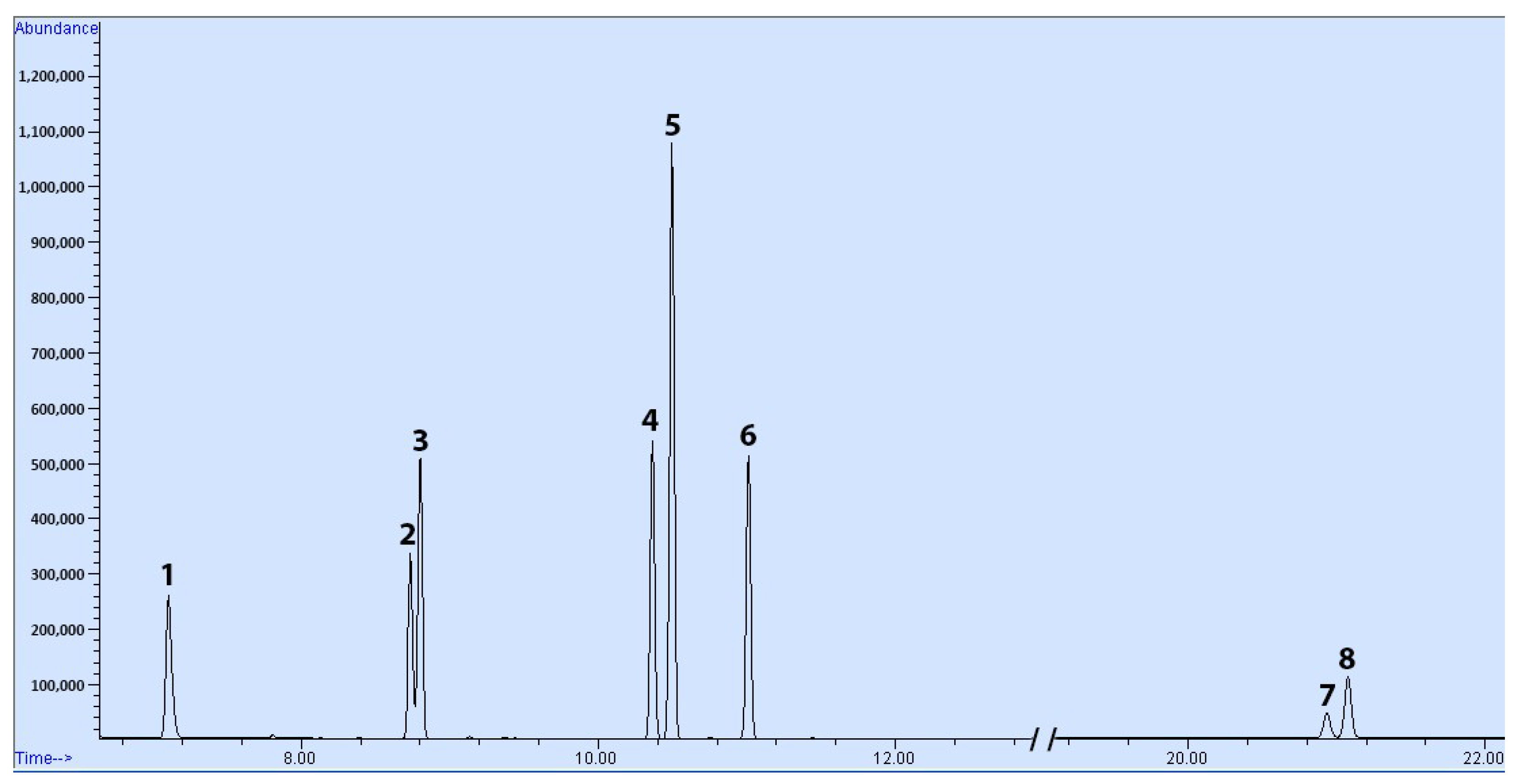
The GC-MS method developed successfully resolved all target compounds with acceptable peak shapes. A representative chromatogram of a spiked sample is shown in Figure 3. In spite of all of the measures, the benzene peaks exhibited a tailing factor of 1.6, likely due to the limited solvent-focusing effect of DCM. Regardless, the tailing remained within acceptable limits, and did not hinder the identification or quantification of benzene. It is worth noting that, as observed in the chromatogram, the column was unable to separate m-xylene from p-xylene; therefore, the method quantifies the combined concentration of both isomers.

3.3. Method Validation

The method validation results are summarized in

Table 1. Summary of method performance characteristics (N—number of samples).

Analyte	Nominal Concentration (µg/L)	N	Average Recovery (µg/L)	Average Recovery (%)	SD (µg/L)	RSD (%)
Benzene	11.51	3 × 10	10.87	94%	0.34	3.1%
	767.2	3 × 10	789.5	103%	20.26	2.6%
Toluene	11.71	3 × 10	10.54	90%	0.22	2.1%
	780.8	3 × 10	778.4	100%	8.55	1.1%
Ethylbenzene	11.78	3 × 10	10.47	89%	0.19	1.8%
	785.6	3 × 10	760.4	97%	9.36	1.2%
m/p-Xylene	23.50	3 × 10	20.53	87%	0.45	2.2%
	1566	3 × 10	1544	99%	29.36	1.9%
o-Xylene	11.78	3 × 10	10.12	86%	0.18	1.8%
	785.6	3 × 10	744.9	95%	9.90	1.3%
Sulfolane	11.93	3 × 10	10.77	90%	0.88	8.1%
	795.2	3 × 10	746.6	94%	3.50	0.5%

. The method demonstrated good selectivity, correctly identifying and accurately quantifying all target compounds in the spiked samples. Recoveries ranged from 86% to 103%, with RSDs between 0.5% and 8.1%. LODs and LOQs were between 0.5 µg/L and 2.6 µg/L, and 1.8 µg/L and 8.8 µg/L, respectively, as shown in

Table 2. Limits of detection and quantification of the analytical method.

	Benzene	Toluene	Ethylbenzene	m/p-Xylene	o-Xylene	Sulfolane
LOD (µg/L)	1.0	0.7	0.6	1.3	0.5	2.6
LOQ (µg/L)	3.4	2.2	1.9	4.5	1.8	8.8

. While lower LODs and LOQs could be achieved by focusing on a single compound class (i.e., BTEX or sulfolane alone), the dissimilar polarities of these analytes necessitated methodological compromises. These included using a 1:1 split injection ratio and selecting a column that could accommodate both compound groups rather than a specialized column for individual analytes. Additionally, sample preparation was kept straightforward, with no preconcentration steps applied. Given these trade-offs, the observed LOD and LOQ values are well within acceptable limits and sufficiently sensitive for their intended purpose, as the current regulatory thresholds for these compounds are higher than the method’s LOQs.

3.4. Method Ruggedness Testing

Method ruggedness can be evaluated by examining how small changes in experimental parameters that might occur during sample preparation and analysis affect the final results. A design of experiments (DOE) approach was implemented to assess the ruggedness of the method, and to identify the most influential factors affecting analytical results. When properly selected, these designs enable efficient optimization by significantly reducing the number of experimental runs required. A 12-run Plackett–Burman design was chosen, as it allows for the evaluation of 11 factors with only 12 experimental runs, making it a highly efficient screening method. However, every experimental design has limitations, and in the case of the Plackett–Burman design, it assumes that interactions between factors are negligible. This assumption must be considered when interpreting the results.

The interpretation of the Plackett–Burman design results is presented in Pareto charts in Figures S1 and S2, with factors included in Table S3. The analyses highlighted the significance of vortex shaking on the response of all compounds except sulfolane. However, when accounting for losses by plotting calibration curves using the ratios of BTEX compounds to toluene-d8 and sulfolane to sulfolane-d8, respectively, none of the compounds, except benzene, appeared to be influenced by the experimental factors tested.

Benzene, even after correction with the surrogate standard, showed significant sensitivity to both the time taken to add the water sample to the DCM and the volume of DCM used. This sensitivity can be attributed to the higher vapor pressure of benzene compared to other BTEX compounds [31]. Its elevated vapor pressure allows for benzene molecules to escape from the water more readily, making delays in handling the sample critical to its concentration. To mitigate this issue, it is recommended to add surrogate standards directly to the DCM and immediately transfer water samples into the DCM in the injection vial upon opening the sample vials.

3.5. Sample Stability Test

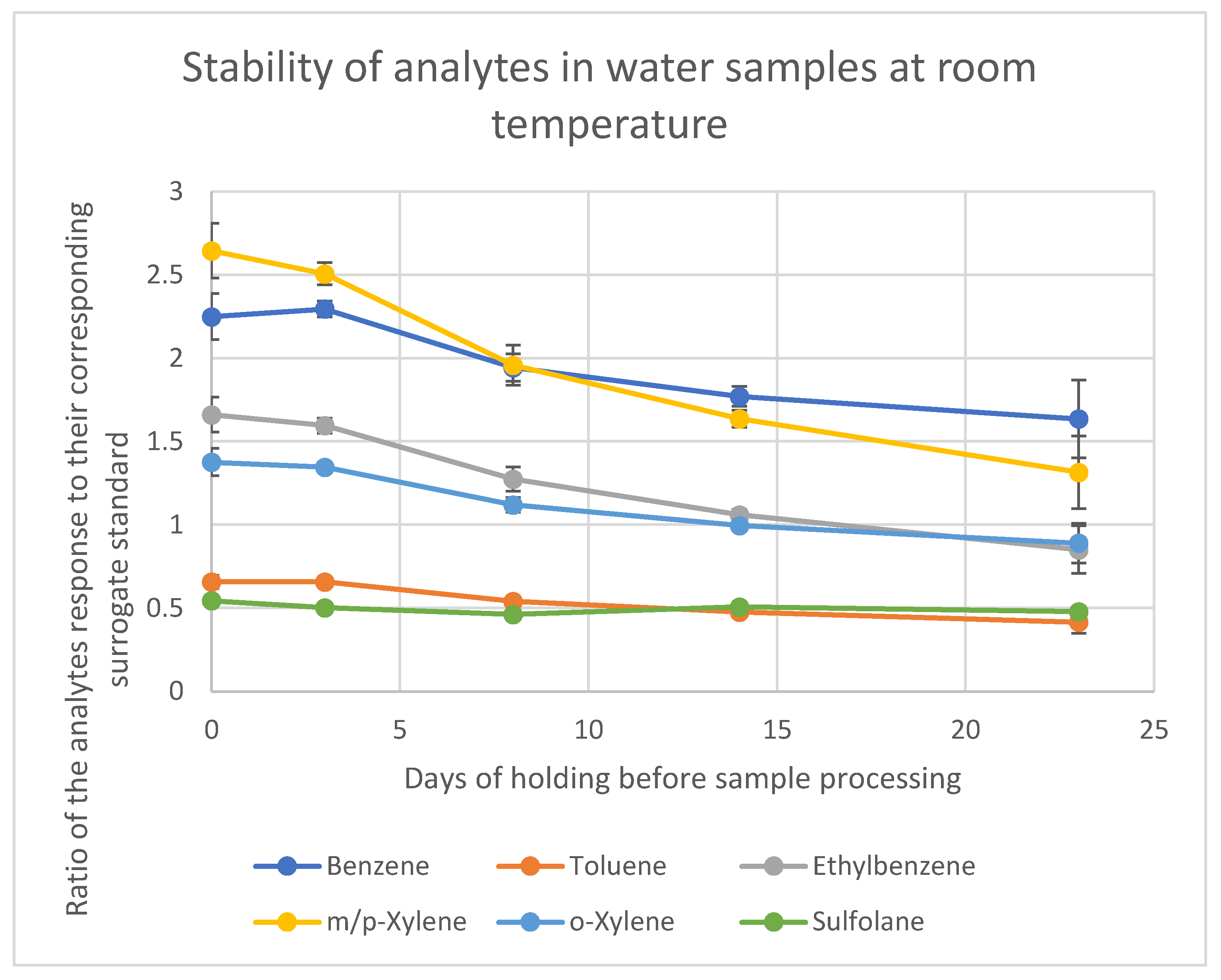
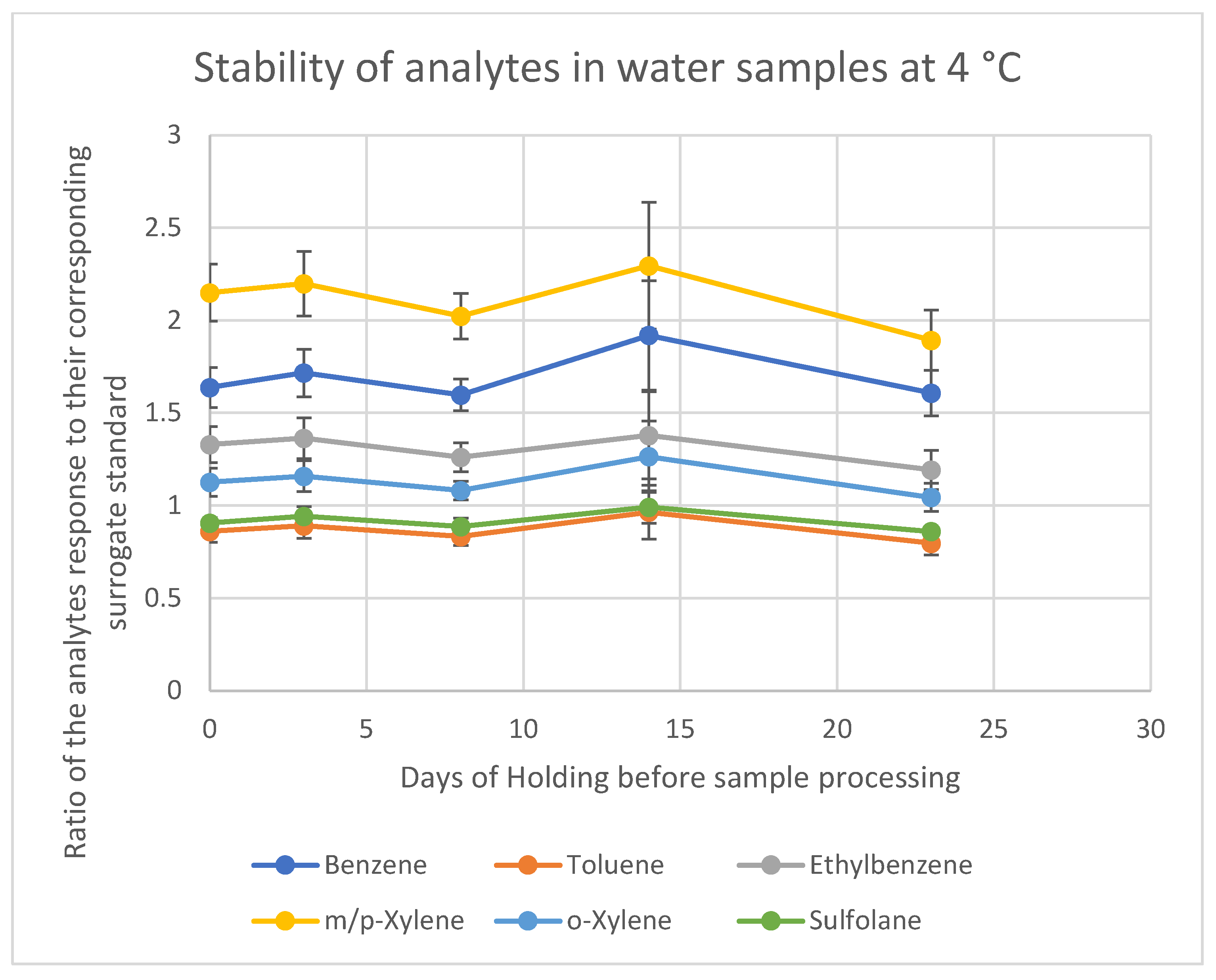
The results for the samples stored at room temperature and 4 °C are summarized in Figure 4 and Figure 5, respectively, with detailed data provided in Tables S4 and S5. For both storage conditions, the data show that sulfolane remains stable for up to 23 days, as expected, given its non-volatile nature and minimal degradation potential in water under these storage conditions. In contrast, the loss of BTEX compounds begins immediately after sample collection if they are stored at room temperature.

For samples stored at room temperature, the most significant losses were observed for m-xylene and p-xylene, which showed a 26% reduction in concentration after 8 days. Ethylbenzene exhibited a 23% loss over the same period. In contrast, samples stored in the refrigerator showed no significant losses up to 23 days. Based on these findings, it is recommended to store water samples in the refrigerator to preserve the target analytes. However, if refrigeration is not feasible, it is essential to process and analyze the samples within 7 days to limit the loss of analytes to less than 25%. All samples collected for this study were stored at 4 °C for a maximum of 7 days; hence, they were deemed stable.

3.6. Analysis of Water Samples

The results of the water sample analyses are presented in Table S6. In most cases, the duplicate samples exhibited consistent results, as expected. Any inconsistencies were carefully examined, with the conclusion that these discrepancies likely resulted from sampling variability rather than analytical determination errors. This variability is unavoidable when working with real-world samples, as obtaining identical duplicates in the field can be challenging. Groundwater samples present a particular challenge, as they must be collected using a pump, leading to variations in collection times. Also, the amount of groundwater that could be drawn from a particular layer of the aquifer was, in some cases, insufficient to fill two vials at the same time. In cases like these, the collection had to be resumed at a different time; hence, the samples could not be treated as true replicates. Finally, the use of a peristaltic pump can influence the concentration of BTEX compounds, since the pump’s internal tubing is made of silicone rubber, which can absorb these analytes. However, the limited contact time and rapid sample collection should help minimize these effects.

The current federal long-term water quality guidelines for the preservation of aquatic life, as defined by Environment and Climate Change Canada, are 0.59 mg/L for benzene, 0.03 mg/L for toluene, and 0.07 mg/L for both ethylbenzene and total xylenes. Similarly, the Government of Alberta sets a maximum level of 0.09 mg/L for sulfolane in groundwater. As shown in

Table 3. Summary of the results of the analysis of water samples.

Contaminant	Benzene	Toluene	Ethylbenzene	m/p-Xylene	o-Xylene	Sulfolane
Positive samples, N	0	6	0	2	0	24
Positive samples, %	0%	12%	0%	4%	0%	48%
Quantified samples, N	0	6	0	2	0	20
Average concentration, positive samples (µg/L)	0.00	70.0	0.00	8.85	0.00	673
Quantified samples above long-term guideline, N	0	3	0	0		17

, 17 samples contained sulfolane at concentrations exceeding the recommended screening level. In contrast, few samples showed detectable BTEX compounds, with only three samples exceeding the long-term guideline concentration for toluene. Environmental factors, including seasonal variations, rainfall, and temperature, may influence these contamination levels. Therefore, regular monitoring is recommended to develop a more comprehensive understanding of the contaminant profile in this area.

4. Conclusions

An analytical method for the simultaneous determination of BTEX and sulfolane in a single run was developed and validated. The method demonstrated good selectivity and sensitivity, with LOQs ranging from 1.8 µg/L to 8.8 µg/L for the analytes in water. The calibration range extended from the LOQ up to 8000 µg/L for all compounds.

Method ruggedness was evaluated using the Plackett–Burman experimental design. Among the factors studied, benzene was significantly affected by the time elapsed between exposing the water sample to air and adding the extraction solvent, highlighting the compound’s volatility.

Sample holding time was assessed at both room temperature and refrigerated conditions by preparing two identical sets of spiked samples and analyzing them over a three-week period. Based on the results, it is recommended to process and analyze samples within 7 days of collection, as BTEX losses exceeded 25% beyond this time frame in the worst case scenario (storage at room temperature).

Finally, the method was used to analyze 97 surface water and groundwater samples from a contaminated site in Alberta, Canada. The analysis indicated that water from 17 out of 50 locations contained sulfolane concentrations above Health Canada’s recommended screening level for drinking water, while two locations exhibited toluene levels exceeding the MAC set by Health Canada. While these results warrant attention, a more comprehensive understanding of the contamination profile at the site and an accurate assessment of the associated risk require analyzing a larger number of samples over time. Overall, the method is suitable for its intended purpose, and effective for monitoring BTEX and sulfolane in water samples.