Service Life Prediction of Concrete Coated with Surface Protection Materials by Ultrasonic Velocity in Cold Region

Abstract

Lithium silicate (LS) crack repairing material, working as a crystal waterproof material, could be used to strengthen concrete made from solid waste materials. This paper presents the results of water absorption and rapid freeze–thaw tests with concrete specimens coated with LS. Concrete specimens with different water–binder ratios and air content (0.35–1 and 0.55–4.5) were tested. The moisture uptake and water absorption coefficient were analyzed in the water absorption test. The water absorption coefficient of LS-coated specimens was lower than that of uncoated specimens, resulting in a lower total moisture content. The relative dynamic modulus of elasticity was calculated by the fundamental transverse frequency (Er) and ultrasonic velocity (Ev), respectively. Er and Ev exhibited similar attenuation characteristics, and the attenuation of LS-coated specimens was lower than that of uncoated specimens. A two-segment freeze–thaw damage model based on Er and Ev was employed to predict the service life of concrete. The relative errors of the service life results calculated by Er and Ev were within 10%. The two-segment freeze–thaw model could be used for the service life prediction of concrete structures. The present work provides new insight into using LS to improve the service life of concrete.

1. Introduction

Concrete is one of the most commonly used building materials in civil engineering. As the urban population continuously increases, the amount of industrial waste is increasing year by year. China, for instance, generates 600 million tons of industrial waste residue and waste ore each year. One promising way to recycle industrial waste in construction is to add the waste during concrete production [1,2,3,4,5]. However, the heterogeneity of the waste is an obstacle to elucidating the durability of waste-containing concrete, resulting in difficulties in predicting the service life of concrete. The service life of concrete structures over time is closely related to interactions with the environment. Extreme environments, for example, those with freeze–thaw cycles, greatly influence concrete construction integrity and thus impair concrete’s service life. The addition of industrial waste during concrete production provides a better intrinsic system of voids in the concrete, leading to better durability to freeze–thaw, since the extra voids can ease the hydraulic pressure. However, the effect of industrial waste on improving freeze–thaw resistance is still not clear since the results often diverge due to the different kinds of waste or different experimental methods [6,7].

The mechanism responsible for concrete damage under freeze–thaw is hydraulic pressure. The water in the capillary pores begins to freeze during freezing, resulting a 9% volume increase [8,9]. The formation of ice forces the unfrozen water to move to the nearby pores. The movement causes hydraulic pressure on the capillary walls, which will result in micro-cracks when the pressure increases beyond the tensile strength [10,11]. The appearance of micro-cracks will destroy the integrity of the concrete and reduce its service life.

Considering the concrete deterioration mechanism, scholars have found ways to enhance concrete’s freeze–thaw resistance during concrete production [12,13]. Falchi found that the addition of silane in concrete preparation did not influence the hydration reaction, and it induced good concrete freeze–thaw resistance [14]. Liu added denitrifying bacteria during concrete production and found that bacteria bonded the ITZ, resulting in enhanced resistance to freeze–thaw [15]. On the other hand, for existing concrete construction, surface protection can provide excellent water-repellent performance and freeze–thaw resistance in concrete. In general, surface protection methods can be classified into two groups: (1) hydrophobic protection, which produces a water-repellent surface and has no pore-filling effect; and (2) filling protection, which fills the cracks and capillaries and thus reduces surface porosity. Hydrophobic protection can alter the concrete surface to make it water-repellent. Under this circumstance, water can be prevented from penetrating the surface of the concrete. In the latter, surface protection material can penetrate the concrete through pores, capillaries, and micro-cracks and react with hydration products to fill in the cracks and pores, thus reducing the porosity and increasing the strength.

The deterioration of concrete structures is caused by chemical attack, environmental effects (such as freeze–thaw), and service loads. Therefore, accurately assessing the service life of concrete is important. Testing methods (such as ultrasonic velocity and fundamental transverse frequency) have been adopted to assess concrete durability [16]. The destructive testing method always causes a reduction of the load-bearing area and is cost-consuming. On the other hand, the nondestructive testing method is easy to conduct. Shang utilized nondestructive testing technology to establish the relationship between the mechanical properties and ultrasonic velocity. The results predicted the service life of existing concrete structures such as offshore platforms and concrete dock walls [17]. Yan compared the service life of concrete predicted using the fundamental transverse frequency method, the ultrasonic velocity method, and the shear wave velocity method. The results showed that all three methods could predict the service life of concrete [18].

Several models have been suggested to determine the resistance of concrete specimens to freeze–thaw. Fagerlund proposed a method to analyze the relationship between the degree of saturation and freeze–thaw deterioration [19]. Cho conducted a regression analysis to predict the freeze–thaw damage of concrete based on the limit state function of the response surface method [20]. Yu set up a new equation aimed at determining the freeze–thaw damage caused by different freeze–thaw media and systems through rigorous theoretical derivation [21]. Chen applied MINITAB to perform a nonlinear regression analysis for fracture energy, and the three-parameter Weibull distribution model was used to predict the service life of the concrete specimens [22]. However, measuring fracture energy is relatively complicated and costly, thus there are few studies that have published freeze–thaw fracture energy damage models. The limited models affected the prediction accuracy of the service life of concrete. Therefore, more research should be conducted to establish damage models for concrete freeze–thaw and to predict the service life of concrete using different damage criteria. The aim of this study was to propose a new way to predict the service life of concrete with high prediction accuracy by creating a two-segment damage model according to the tendencies of the fundamental transverse frequency and ultrasonic velocity.

In this study, the effect of the surface treatment material lithium silicate (LS) on concrete freeze–thaw resistance was determined using water absorption and rapid freeze–thaw tests. In the water absorption test, the weight gain was measured during the test, and the moisture uptake and coefficient of water absorption were calculated to clarify the effect of LS on preventing water from penetrating the concrete specimens. For the rapid freeze–thaw test, the relative dynamic modulus of elasticity was calculated by the fundamental transverse frequency (Er) and ultrasonic velocity (Ev), respectively, in order to evaluate the concrete damage due to the conducted freeze–thaw cycles. In addition, a two-segment damage model was adopted to predict the service life of concrete. The model for predicting concrete’s service life was verified by comparing the service life results calculated by Er and Ev, which provided an effective calculation basis for the design of freeze–thaw resistant concrete.

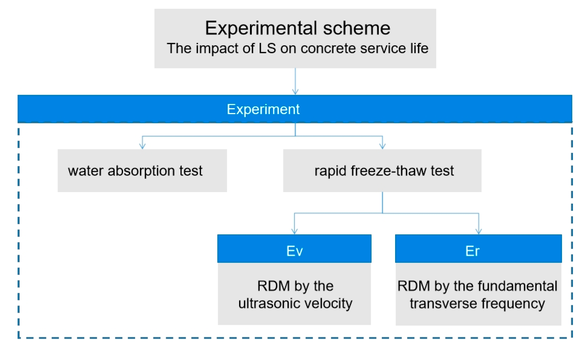
2. Materials and Methods

2.1. Raw Materials

In the experiment, the binder was P.O. 42.5 Portland cement. It had a specific surface area of 332 m²/kg and the chemical components are shown in

Table 1. Chemical components of cement (wt.%).

Chemical Composition (wt.%)
Oxides	CaO	SiO2	Al2O3	Fe2O3	SO3	MgO	Na2O	K2O	Others
Content	61.10	22.70	6.85	2.86	3.61	0.95	0.36	0.28	3.88

. The fine aggregate was silica sand with a fineness modulus of 2.43, and the density was 2.6 g/cm³. The coarse aggregate was limestone with a nominal maximum size of 25 mm.

This investigation studied the effect of LS on enhancing the service life of different kinds of concrete specimens. Two commonly used water/cement ratios, 0.35 and 0.55, were adopted. In addition, air entrainment is used especially against freeze–thaw attack. In order to obtain adequate freeze–thaw resistance, a certain air content (4–6%) is needed according to previous studies. For better comparison of the effect of LS on concrete’s service life, air contents of 1% and 4.5% were employed. Two commercially available admixtures (air entrainer and defoamer) were adopted. The air entrainer was used at a dosage of 4.0 mL/kg cement material. The air defoamer dosage was maintained at 1.2 mL/kg cement material. The mix proportions are listed in

Table 2. Concrete mix proportions.

Mix	Mix Proportion (kg/m3)				External Coating
	Cement	Sand	Limestone	Water
0.35–1.0–LS	471	827	978	165	LS
0.35–1.0–NO					None
0.55–4.5–LS	313	843	949	172	LS
0.55–4.5–NO					None

. All mixtures were mixed in a concrete mixer in accordance with the ASTM C 192 procedure. After mixing, the mixtures were filled into the molds. All specimens were removed from the molds after one day and then submerged in tap water at 20 °C for another 27 days.

In each mix proportion, two cylinder specimens of Φ100 × 200 were obtained from the molded cylinder according to Practice C 31M. Then, 3 cylinder samples with the size of Φ100 × 50 were cut out from each mix proportion. These cylinder samples underwent the concrete water absorption test, in accordance with ASTM C1585. Three concrete prism specimens of 100 × 100 × 400 were also fabricated in each mix proportion. The prism specimens were used to conduct the rapid freeze–thaw test according to Chinese specification GB/T 50082-2009.

The surface protection product (LS) used in this study was an inorganic lithium silicate-based impregnation, which could penetrate the concrete specimens and react with the concrete hydration products to fill the cracks and pores. This product is commercially available and often applied to protect concrete substrates. For the specimens coated with LS, the surfaces of the concrete specimens were wet and sprayed with LS. All of the surfaces were uniformly and carefully sprayed. The surfaces were sprayed again when the surfaces were dry. After curing for 24 h, the surfaces of the specimens were cleaned with water. Further, the comparison specimens were all kept at room temperature until the experiment.

For the mix denotation (e.g., 0.35–1–LS), the first two parameters indicate the w/b ratio and air content, respectively, while the last parameter is the external coating condition of the hardened concrete specimen.

2.2. Experimental Procedures

The experiment comprised water absorption and rapid freeze–thaw tests. The water absorption test was used to clarify the effect of LS on enhancing the concrete’s water absorption ability. The rapid freeze–thaw test was employed to determine the change in the relative dynamic modulus calculated by the fundamental transverse frequency and the ultrasonic velocity, respectively. Figure 1 shows the configuration of the experiment.

2.2.1. Water Absorption Test

The resistance of the two specimen types to water impregnation was evaluated by the water absorption test according to ASTM C 1585, where the water absorption was measured by the weight increase. The cylinder samples were dried in the oven at 50 °C until a constant weight was achieved. Aluminum foil was used to seal the lateral surfaces with epoxy resin. Subsequently, a one-week moisture uptake test was conducted under isothermal conditions (20 °C) in demineralized water and the weight change was measured at suitable time intervals. The experimental regime ensured the saturation of the connected capillary pores. The disconnected and air-entrained pores were slowly filled by diffusion throughout the water absorption test [19]. Figure 2 shows the setup of the water absorption test.

When concrete is exposed to water, water can penetrate the concrete through capillary pressure. Water absorption is related to many durability-related problems, e.g., chloride penetration, damage to the concrete structure [23,24,25]. Water absorption was measured through the specimen’s weight gain. The coefficient of water absorption was determined by the changing rate of the linear water absorption curve during the beginning of the water absorption test. The following formulas were used to calculate the water absorption coefficient [23,26]:

$$\Delta \mathrm{W}(t)=\alpha \times \left[1-\exp (-\beta \sqrt{t})\right]$$

(1)

$$\mathrm{B}(t)=\frac{\mathrm{d}\Delta W}{\mathrm{d}(\sqrt{t})}=B_{ini}\times \exp (-\beta \sqrt{t})$$

(2)

where ΔW is the weight gain per unit area, t is the water absorption time, B is the coefficient of water absorption, and B_ini is the initial coefficient of water absorption, where B_ini = α × β.

2.2.2. Rapid Freeze–Thaw Test

The rapid freeze–thaw test was carried out according to Chinese specification GB/T 50082-2009. In the test, the lowest temperature was −18 ± 2 °C and the highest temperature was 5 ± 2 °C. In each freeze–thaw cycle, the freezing regime was completed within 2.5 h and the thawing regime was no more than 1.5 h.

The relative dynamic modulus of elasticity by the fundamental transverse frequency (Er) is an important factor to clarify mechanical performance degradation. E_r was evaluated according to the following formula:

$$E_r=\frac{M_{r-t}}{M_{r-0}}=\frac{f_t^2}{f_0^2}$$

(3)

where M_r−0 is the initial dynamic modulus of elasticity, M_r−t is the dynamic modulus of elasticity after t cycles, f₀ is the initial fundamental transverse frequency, and f_t is the fundamental transverse frequency after t cycles.

Freeze–thaw damage to concrete specimens results in the decline of the dynamic modulus of elasticity due to a process of degradation inside the concrete [27]. The degree of damage to the concrete during freeze–thaw cycles can be defined by the formula below based on the damage mechanics:

$$D=\frac{M_{r-0}-M_{r-t}}{M_{r-0}}=1-E_r$$

(4)

where D is the freeze–thaw damage degree.

The ultrasonic velocity was measured using a concrete ultrasonic detector. A concrete ultrasonic detector has been widely used to check the quality of concrete by passing ultrasonic waves through the concrete. The frequency range was set between 20 and 100 kHz, and the interval was 1 μs. A dynamic elastic modulus tester produced by NELD-DTV Company was used to calculate the fundamental transverse frequency. The ultrasonic wave velocity and fundamental transverse frequency of the concrete specimens were measured at every 25 freeze–thaw cycles (0, 25, 50, 75, 100, …, 300).

3. Results

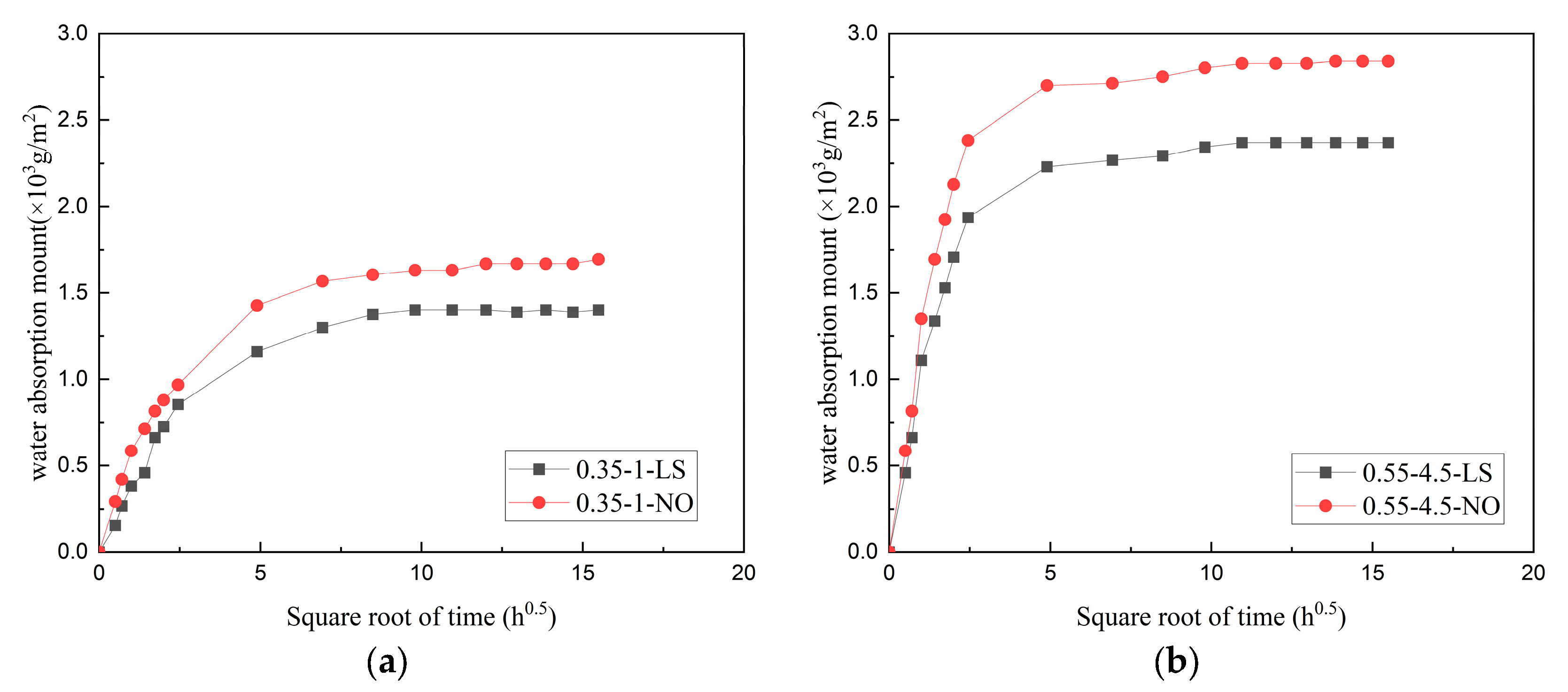
3.1. Results of the Water Absorption Test

Figure 3 presents the results of water absorption uptake against time. According to Figure 3, the variation in the water absorption trends of the two types of concrete specimens (0.35–1, 0.55–4.5) increased in a similar manner. The water absorption curve comprised two distinguished polynomial patterns: the first pattern was a rapid and linear increase, while the latter was a smooth transition. The rapid increase part was attributed to rapid capillary absorption, while the soft transition part was the result of slow uptake by diffusion [28].

Table 3. Variation of concrete samples in the water absorption test.

Sample	α	β	Bini = α × β	Total Water Absorption (%)
0.35–1–NO	1.45	0.80	1.16	1.69
0.35–1–LS	1.30	0.58	0.75	1.40
0.55–4.5–NO	2.82	0.64	1.80	2.84
0.55–4.5–LS	2.34	0.60	1.40	2.34

displays the coefficient of water absorption and the total water absorption of the two types of concrete specimens. In the first pattern, the values of the initial coefficient of water absorption (B_ini) of the four concrete groups (0.35–1–NO, 0.35–1–LS, 0.55–4.5–NO, 0.55–4.5–LS) were 1.16, 0.75, 1.80, and 1.40, respectively. The B_ini values of the LS-sprayed specimens were smaller than those of the unsprayed specimens for both the 0.35–1 and 0.55–4.5 specimens. In addition, the total water absorption amounts of the four concrete groups were 1.69%, 1.40%, 2.84%, and 2.34%, respectively. As exhibited in Figure 3, at the same condition, the amount of absorbed water for the LS-sprayed specimens was smaller than that for the unsprayed specimens. This phenomenon was evident in the 0.55–4.5 specimens. This may have been due to the low w/b ratio of the 0.35–1 specimens and thus their lower porosity. The results were consistent with the results reported by Baltazar [28].

One significant implication of the differential water absorption coefficient and total water absorption amount is that the filling of the cracks and air pores was governed by the chemical product of LS reacting with cement hydration products (CHs). Theoretically, the chemical reaction between the LS surface protection material and CHs is expressed as Li₂O∙nSiO₂ + mH₂O + nCa(OH)₂→nCaO∙SiO₂∙(m + n−)H₂O + 2LiOH. LS reacts with part of the CHs to form new C-S-H, which densifies the concrete surface. Therefore, a slow water absorption coefficient, B_ini, and a lower total water absorption amount was found in the specimens coated with LS.

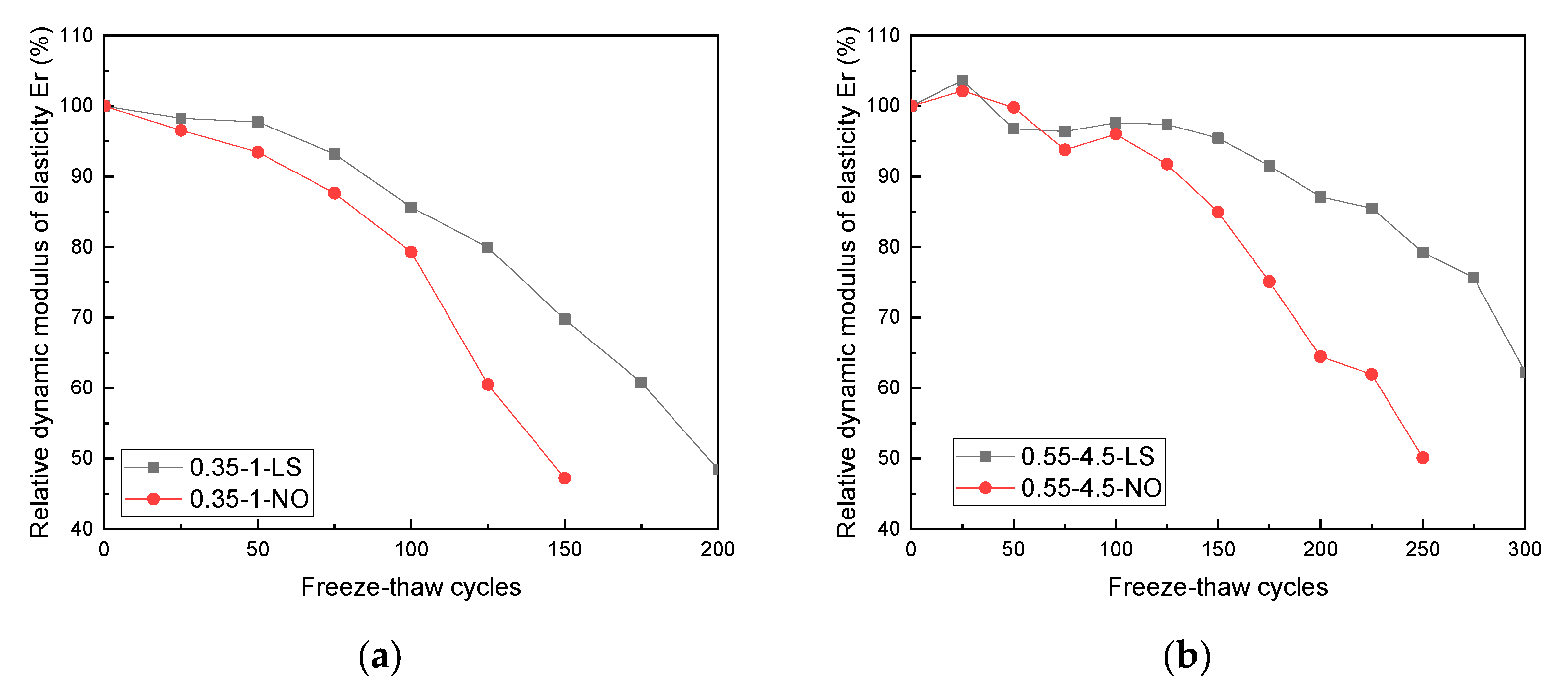
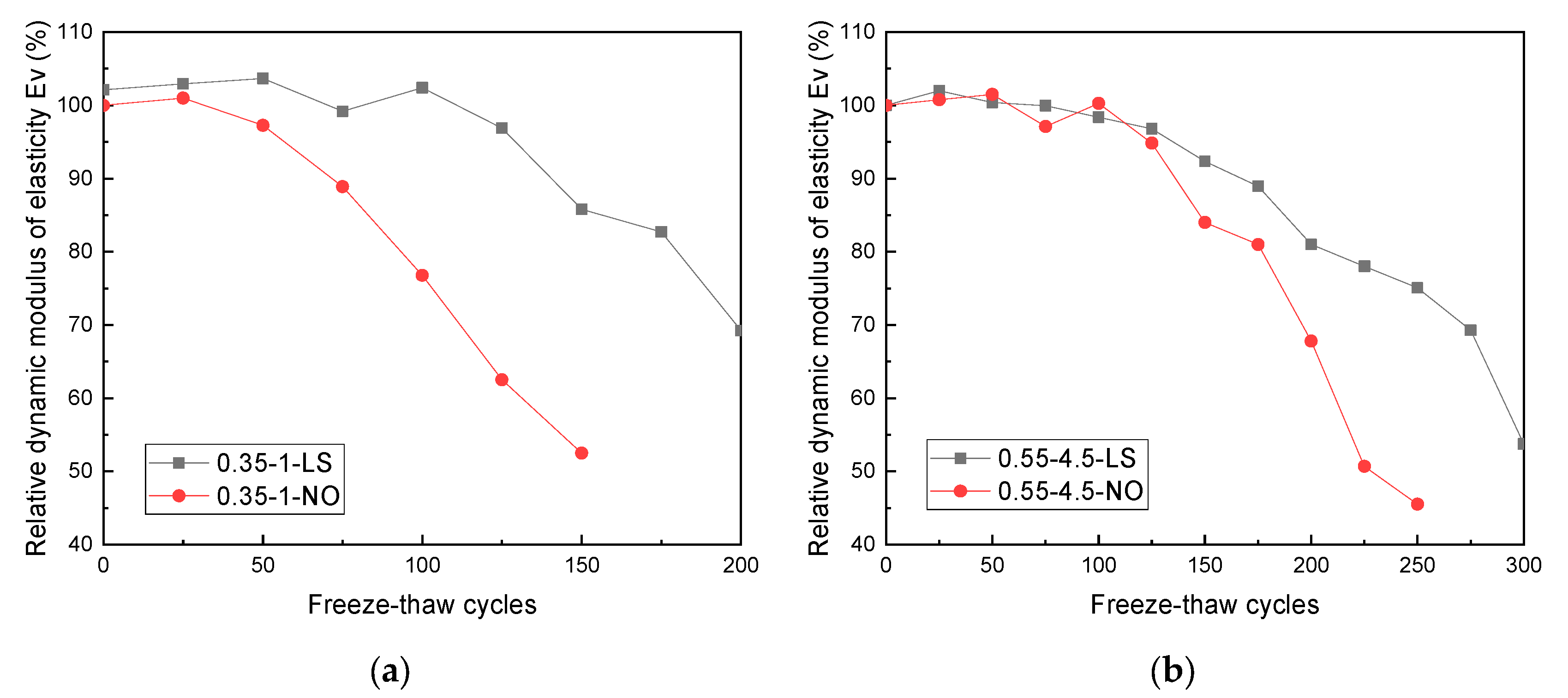
3.2. Results of the Relative Dynamic Modulus of Elasticity

Figure 4a,b exhibits the change in E_r with freeze–thaw cycles, assuming a 60% cut-off limit. It can be seen from Figure 4a that the E_r of the 0.35–1–NO specimens decreased slowly before 50 cycles and then displayed a rapid decrease afterwards. At 150 freeze–thaw cycles, the E_r of the 0.35–1–NO specimens was 46.06%, surpassing the failure criterion according to Chinese specification GB/T 50082-2009. On the other hand, the E_r of the 0.35–1–LS specimens showed a similar tendency compared to the 0.35–1–NO specimen, reaching the failure criterion of 48.62% at 200 freeze–thaw cycles. The LS-coated specimens showed better freeze–thaw resistance. Figure 4b demonstrates the E_r tendency of the concrete specimens (0.55–4.5–NO, 0.55–4.5–LS). The E_r of the 0.55–4.5 specimens increased slightly in the early stage of the freeze–thaw cycles. This was because concrete is a heterogeneous composite material with many inherent defects and high porosity. According to Powers’ hydrostatic pressure theory [27], part of the solution in the pores freezes and expands during freezing, forcing the unfrozen solution to migrate out of the pores, therefore discharging the air in the micro-pores. However, external water solution enters the micro-pores and circulates within them when the temperature is positive. The air in the micro-pores is gradually replaced by the water solution. Thus, the mass of the concrete increases and the specimen seems to be denser. This results in a slight increase in the E_r, especially for air-entrained specimens. As shown in Figure 4b, the tendency of the 0.55–4.5–LS specimens was similar to that of the 0.55–4.5–NO specimens before 100 cycles. However, after that, an obvious decrease was found in the 0.55–4.5–NO specimens. The 0.55–4.5–LS specimens displayed more negligible attenuation than the 0.55–4.5–NO specimens. The E_r of the 0.55–4.5–LS specimens at 300 freeze–thaw cycles was 62.23%, while the E_r of the 0.55–4.5–NO specimens at 250 freeze–thaw cycles was 49.32%, which had already reached the damage criterion. Therefore, LS could improve the freeze–thaw resistance in both kinds of concrete specimens.

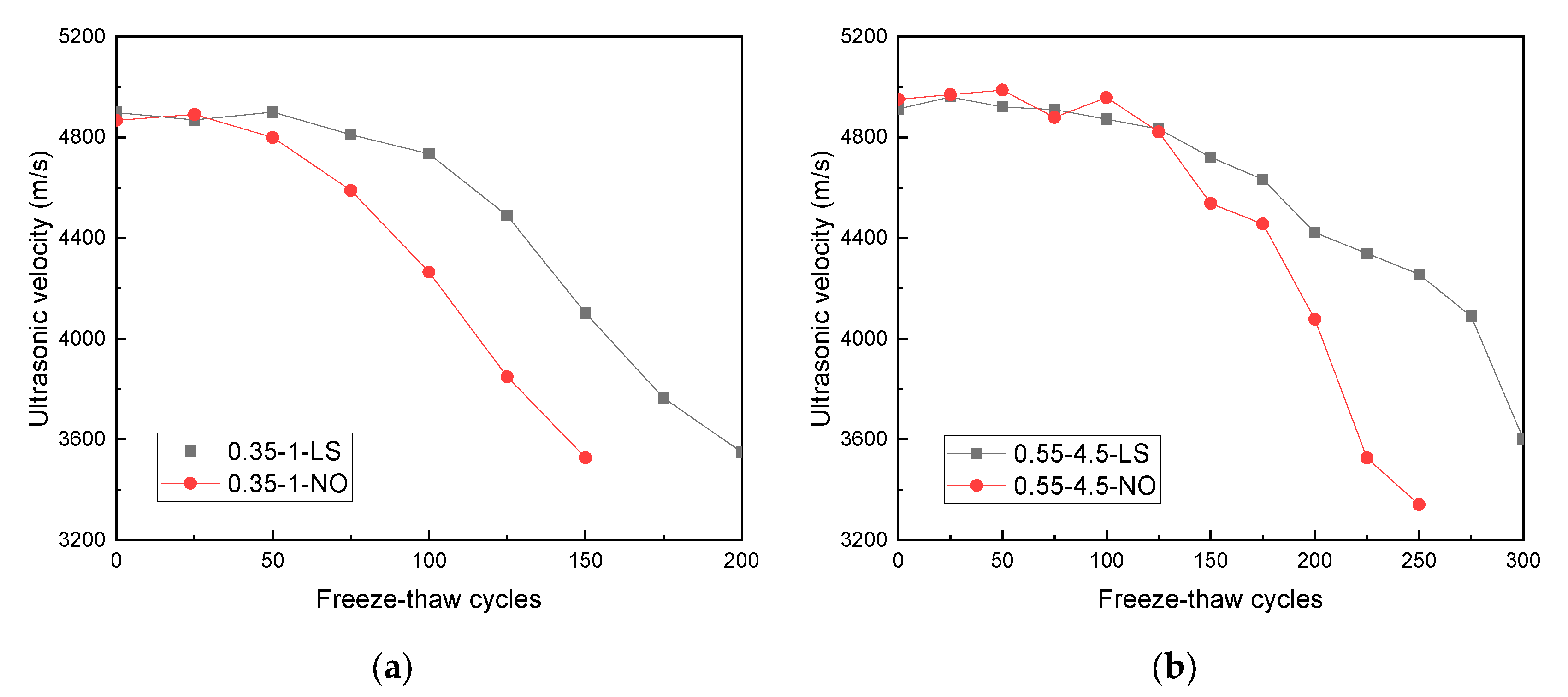
3.3. Change in the Ultrasonic Velocity

The changes in ultrasonic velocity, also known as P-wave velocity, are exhibited in Figure 5a,b. According to Figure 5a, the variation in ultrasonic velocity of the 0.35–1 specimens was slight before 50 freeze–thaw cycles, then it significantly decreased. Compared to the ultrasonic velocity of the 0.35–1–LS specimens, the ultrasonic velocity of the 0.35–1–NO specimens manifested a more pronounced decrease after 50 cycles. In Figure 5b, the ultrasonic velocities for both the 55–4.5–NO and 55–4.5–LS specimens displayed a slight decline before 100 freeze–thaw cycles. The ultrasonic velocity of the 0.55–4.5–NO specimens decreased dramatically after 100 freeze–thaw cycles. On the other hand, the ultrasonic velocity of the 0.55–4.5–LS specimens manifested a smaller attenuation. The ultrasonic velocity results of the 0.55–4.5 specimens corresponded with those of the 0.35–1 concrete specimens. Applying LS surface coating material could delay the attenuation of the ultrasonic velocity during the rapid freeze–thaw test.

The relationship between the dynamic modulus of elasticity M_v and the ultrasonic velocity V has been clarified theoretically according to Equation (5):

$$M_v=\frac{\rho {(1+\mu )}^3}{{(0.87+1.12\mu )}^2}\times {\mathrm{V}}^2$$

(5)

where M_v is the dynamic modulus of elasticity calculated by the ultrasonic velocity, ρ is the specimens density, μ is Poisson’s ratio, and V is the ultrasonic velocity. Since ρ and μ have negligible change, the relative dynamic modulus of elasticity calculated by ultrasonic velocity (E_v) [29,30] is calculated according to Equation (6):

$$E_v=\frac{M_v{}_{-t}}{M_v{}_{-0}}=\frac{V_t^2}{V_0^2}$$

(6)

where M_v−0 and M_v−t are the dynamic modulus of elasticity at 0 cycles and after t cycles, respectively; and V₀ and V_t are the ultrasonic velocity at 0 cycles and after t cycles, respectively.

Figure 6 displays the relationship between E_v, and freeze–thaw cycles. As exhibited in Figure 6a, the E_v of the 0.35–1 concrete specimens decreased slowly before 50 cycles and showed rapid attenuation after 50 cycles. The E_v of the 0.35–1–LS specimens was 67.48% at 200 freeze–thaw cycles, and at 150 freeze–thaw cycles, the E_v of the 0.35–1–NO specimens was 52.52%. The variation trends of E_v were similar to those of E_r. Before 100 freeze–thaw cycles, the attenuation of E_v was small for the 0.55–4.5 concrete specimens, as exhibited in Figure 6b. Nevertheless, E_v decreased quickly after 100 freeze–thaw cycles, ending with 52.77% at 300 cycles for the 0.55–4.5–LS concrete specimens and 44.83% at 250 cycles for the 0.55–4.5–NO concrete specimens, respectively. The E_v and E_r for the 0.55–4.5 specimens exhibited a similar tendency. The E_v of the concrete specimens coated with LS displayed a slower attenuation.

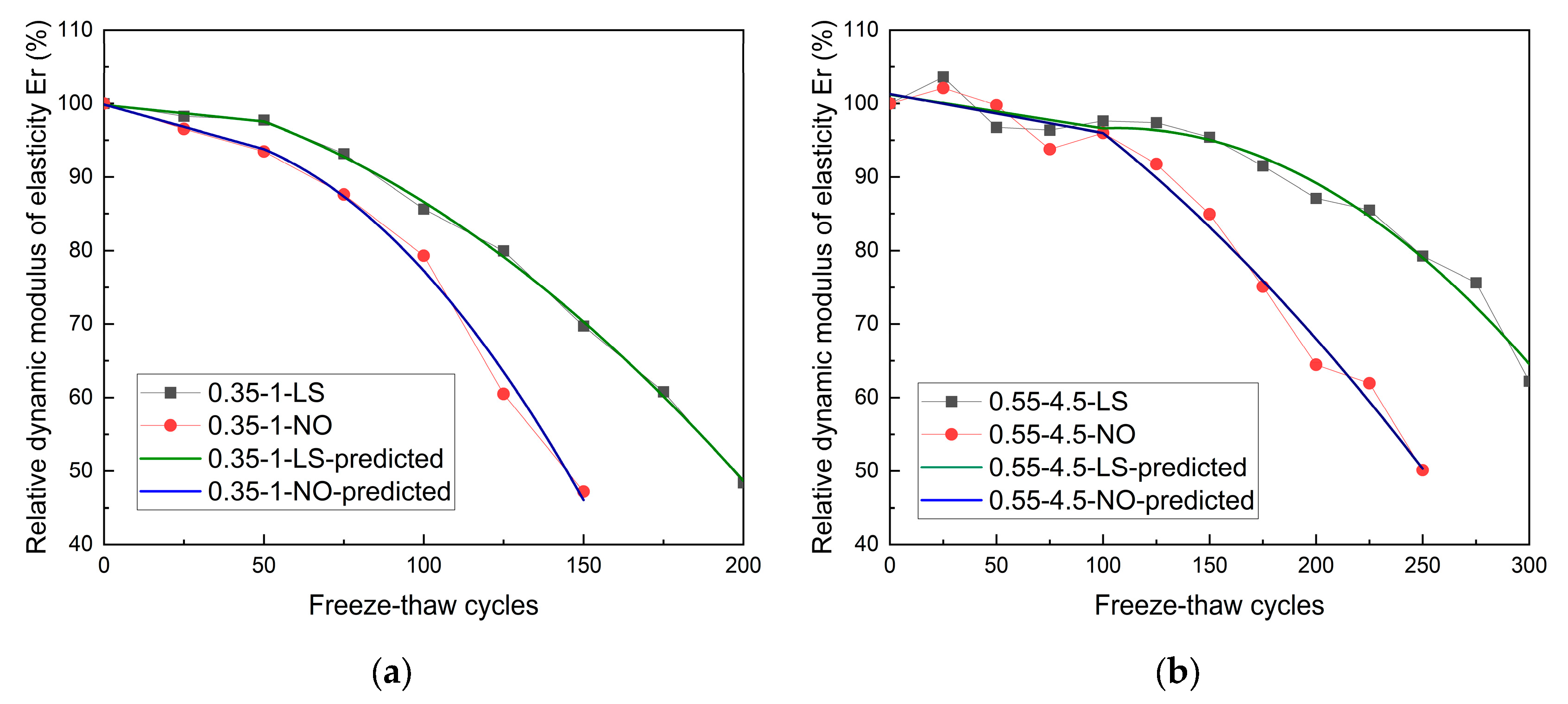
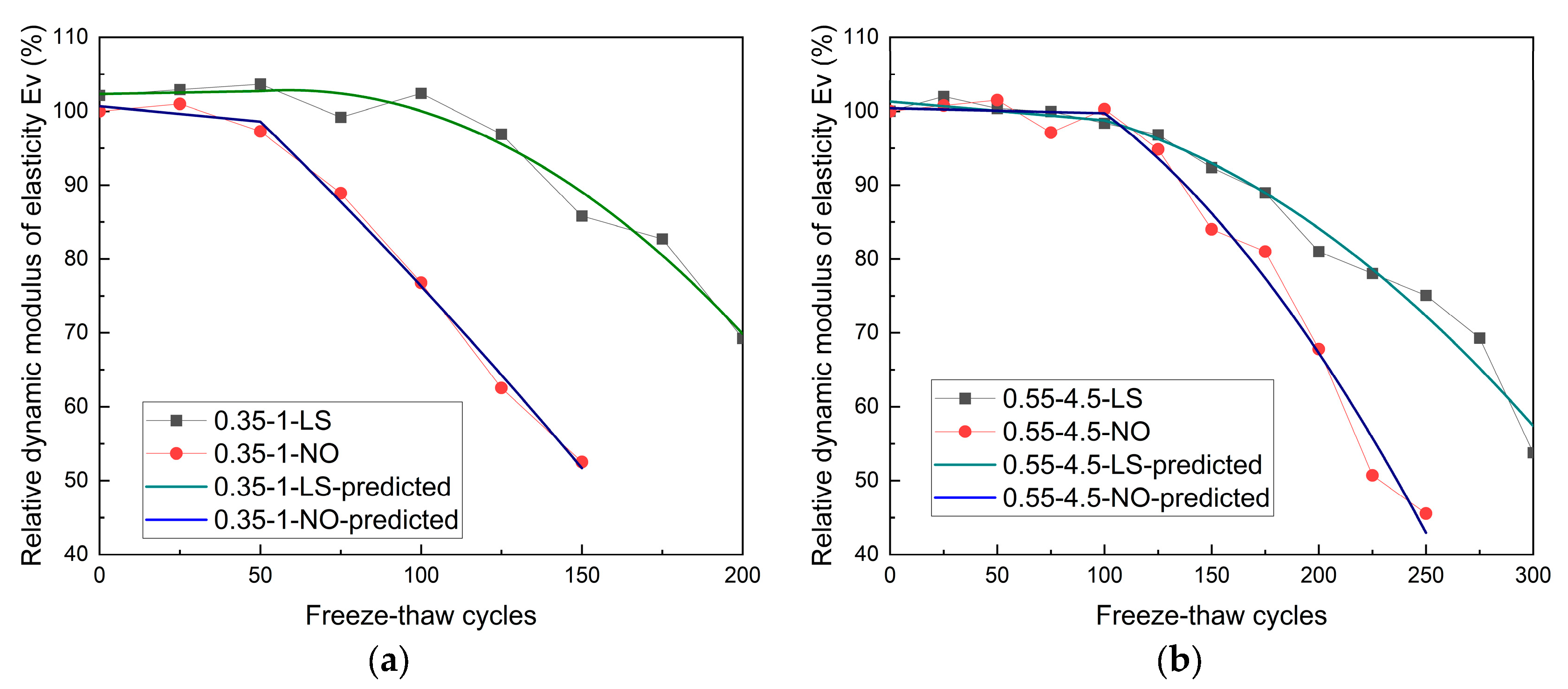
3.4. Prediction of Relative Dynamic Modulus of Elasticity

Many scholars have analyzed the degree of freeze–thaw damage to concrete by establishing different mathematical models [31,32,33]. A two-segment damage mathematical relationship has been employed to characterize the relative dynamic modulus of elasticity [34]. The two-segment damage mathematical model comprises a straight line and a univariate quadratic polynomial. The first segment is a straight line and the second segment is a univariate quadratic polynomial. In this model, there is one tangent point, cycle N₁₂, between the straight line and the univariate quadratic polynomial. The relationship between the relative dynamic modulus of elasticity, E, and the freeze–thaw cycles, N, is described below:

$$\left\{\begin{array}{ll}➀E_1=1+aN& \hfill (N<N_{12})\\ ➁E_2=1+\frac{{(b-a)}^2}{2c}+bN+\frac{1}{2}c{N}^2& \hfill (N>N_{12})\end{array}\right\}$$

(7)

where E₁ represents the straight line, and E₂ represents the univariate quadratic polynomial.

Since concrete damage proceeds during the freeze–thaw test, E also decreases with the freeze–thaw cycles. The univariate quadratic polynomial also exhibits a descending tendency. According to the properties of the univariate quadratic polynomial, the coefficient c should be prior to 0. To better explain the formula, the following derivation is conducted based on Equations (4) and (7). The relationship between the degree of freeze–thaw damage, D, and the freeze–thaw cycles is exhibited below:

$$\left\{\begin{array}{ll}➀D_1=-aN& \hfill (N<N_{12})\\ ➁D_2=-\frac{{(b-a)}^2}{2c}-bN-\frac{1}{2}c{N}^2& \hfill (N>N_{12})\end{array}\right\}$$

(8)

(1)

In the first segment ①, the velocity and acceleration are shown as follows:

$$\left\{\begin{array}{l}\frac{dD}{dN}\left|{}_{N<N_{12}}\right.=-\frac{d{E}_{r1}}{dN}\left|{}_{N<N_{12}}\right.=-a\\ \frac{d^{2}D}{d{N}^2}\left|{}_{N<N_{12}}\right.=-\frac{d^2{E}_{r1}}{d{N}^2}\left|{}_{N<N_{12}}\right.=0\end{array}\right\}$$

(9)

where the velocity is −a and the acceleration rate is 0, respectively. Thus, the first segment is a uniform damage period.

(2)

In the second segment ②, the velocity and acceleration rate are exhibited as below:

$$\left\{\begin{array}{l}\frac{dD}{dN}\left|{}_{N>N_{12}}\right.=-\frac{d{E}_{r2}}{dN}\left|{}_{N>N_{12}}\right.=-(b+cN)\\ \frac{d^{2}D}{d{N}^2}\left|{}_{N>N_{12}}\right.=-\frac{d^2{E}_{r2}}{d{N}^2}\left|{}_{N>N_{12}}\right.=-c\end{array}\right\}$$

(10)

where the velocity is –(b + cN), and the acceleration rate is −c. The second segment is a uniformly accelerated degradation process.

N₁₂ is the freeze–thaw cycle number at the tangent point of the straight line and the univariate quadratic polynomial. The first and second segments should have the same damage velocity at the tangent point N₁₂, that is $\frac{dD}{dN}\left|{}_{N=N_{12}}\right.=-\frac{d{E}_{r1}}{dN}\left|{}_{N=N_{12}}\right.=-(b+c{N}_{12})=-a$. Therefore, N₁₂ is calculated by the coefficients a, b, and c, respectively. Moreover, the damage acceleration changes from 0 to − at the tangent point N₁₂. Concrete freeze–thaw damage changes from uniform damage mode in segment ① to uniform degradation mode in segment ② at the tangent point N₁₂. Thus, N₁₂ is the damage mode changing point.

3.4.1. Prediction of the Relative Dynamic Modulus of Elasticity E_r

According to the two-segment model, the freeze–thaw damage evolution of E_r is fitted by the two-segment damage model, as shown according to Equation (11) below:

$$\left\{\begin{array}{l}{E}_{r1-(0.35-1-LS)}=99.7901-0.045\times N\\ E_{r2-(0.35-1-LS)}=103.1064-0.0577\times N-0.0011\times N^2\\ E_{r1-(0.35-1-NO)}=99.8536-0.1215\times N\\ E_{r2-(0.35-1-NO)}=95.6377+0.1095\times N-0.0029\times N^2\\ E_{r1-(0.55-4.5-LS)}=101.2288-0.0463\times N\\ E_{r2-(0.55-4.5-LS)}=86.8218+0.1838\times N-0.0009\times N^2\\ E_{r1-(0.55-4.5-NO)}=101.2993-0.0532\times N\\ E_{r2-(0.55-4.5-NO)}=114.1774-0.1330\times N-0.0011\times N^2\end{array}\right\}$$

(11)

The results of the predicted Er by the two-segment damage model are displayed in Figure 7a,b. For the 0.35–1 specimens, the tangent freeze–thaw cycle number was set as 50. Meanwhile, for the 0.55–4.5 specimens, the tangent freeze–thaw cycle number was 100. E_r could be well fitted by the two-segment damage model.

Table 4. Parameters of Er calculated by the two-segment damage model.

Specimen Type	Segment 1	Segment 2		Goodness of Fitting (R2)
	Velocity	Damage Velocity	Damage Acceleration
0.35–1–LS	0.045	0.0577 + 0.0022 × N	0.0022 × N	0.9989
0.35–1–NO	0.1215	−0.1095 + 0.0058 × N	0.0058 × N	0.9939
0.55–4.5–LS	0.0463	−0.1838 + 0.0018 × N	0.0018 × N	0.9721
0.55–4.5–NO	0.0532	0.1330 + 0.0022 × N	0.0022 × N	0.9858

shows the calculated velocity in segment 1, the velocity and acceleration rate in segment 2, and the goodness of fit (R²) of the 0.35–1 and 0.55–4.5 concrete specimens. The R² values of the specimens were all above 0.97, representing perfect fitness. The velocity in segment 1 and acceleration rate in segment 2 were above zero, indicating that the concrete freeze–thaw damage had been accelerated. The LS-coated specimens showed a smaller velocity than the uncoated specimens in segment 1. As shown in Figure 7b, the velocity of the LS-coated specimens was 0.0463, while the value of the uncoated specimens was 0.0532. In addition, the damage acceleration was lower for the LS-coated specimens, which verified that LS surface protection could improve freeze–thaw resistance.

3.4.2. Prediction of Relative Dynamic Modulus of Elasticity E_v

The relative dynamic modulus of elasticity E_v of the two types of concrete specimens (0.35–1 and 0.55–4.5) were also according to the two-segment damage model, as exhibited in Equation (12) below:

$$\left\{\begin{array}{l}{E}_{v1-(0.35-1-LS)}=102.3304+0.0079\ast N\\ E_{v2-(0.35-1-LS)}=97.1923+0.1934\ast N-0.0017\ast N^2\\ E_{v1-(0.35-1-NO)}=100.6766-0.0417\ast N\\ E_{v2-(0.35-1-NO)}=118.511-0.3749\ast N-0.0005\ast N^2\\ E_{v1-(0.55-4.5-LS)}=101.3054-0.0254\ast N\\ E_{v2-(0.55-4.5-LS)}=101.2657+0.0356\ast N-0.0006\ast N^2\\ E_{v1-(0.55-4.5-NO)}=100.4121-0.0068\ast N\\ E_{v2-(0.55-4.5-NO)}=110.6278-0.0011\ast N-0.0012\ast N^2\end{array}\right\}$$

(12)

Figure 8 shows the calculated results of E_v.

Table 5. Parameters of Ev calculated by the two-segment damage model.

Specimen Type	Segment 1	Segment 2		Goodness of Fitting (R2)
	Initial Velocity	Damage Velocity	Damage Acceleration
0.35–1–LS	−0.0079	−0.1934 + 0.0034 × N	0.0034 × N	0.9697
0.35–1–NO	0.0417	0.3749 + 0.0010 × N	0.0010 × N	0.9958
0.55–4.5–LS	0.0254	−0.0356 + 0.0012 × N	0.0012 × N	0.9804
0.55–4.5–NO	0.0068	0.0011 + 0.0024 × N	0.0024 × N	0.9853

shows the damage velocity, the damage acceleration, and the goodness of fit (R²). The tangent freeze–thaw cycle numbers for the 0.35–1 and 0.55–4.5 concrete specimens were also fixed at 50 and 100, respectively. According to Table 5, R² was above 0.98, showing an excellent fitting result. It can be seen that the acceleration rate of the two types of specimens were above 0, and the freeze–thaw damage of the specimens was accelerated in the second segment. Only the initial velocity of the 0.35–1–LS specimens was slightly below 0 at −0.0079; the initial velocities of all the other specimens were above 0.

3.5. Calculation of the Service Life by the Two-Segment Damage Model

According to the “Test method for long-term performance and durability of concrete,” concrete is regarded as damaged when the E_r is below 60%. Many scholars have used the E_v to characterize freeze–thaw damage. Chen found that the relative dynamic modulus of elasticity by ultrasonic velocity (E_v) could represent the damage caused by the coupled sulphate and freeze–thaw attack [35].

Similar to the damage criterion defined by the E_r, concrete specimens become deficient when the E_v is below 60%. The service life results of the concrete specimens calculated by E_r and E_v are exhibited in

Table 6. Service life of concrete calculated by E_r and E_v.

Specimen Type	Service Life of Concrete Specimens (Freeze–Thaw Cycles)
	Er	Ev	Error (%)
0.35–1–LS	173	215	24.28
0.35–1–NO	131	132	0.76
0.55–4.5–LS	302	293	2.98
0.55–4.5–NO	222	205	7.66

. As displayed in Table 6, the service life results calculated by E_r and E_v were close to each other. Only the error of the 0.35–1–LS specimens was relatively large at 24.28%, while all the other errors were small, at less than 8%. The authors supposed that the freeze-thaw resistance of the 0.35–1 concrete specimens was relatively low. After spraying with LS, the micro-cracks in the surfaces were reduced, making the specimen’s surface denser. A denser specimen surface facilitates ultrasonic transmission, resulting in a higher service life prediction. After spraying with LS, the E_v of the 0.35–1 specimens increased from 132 to 215, showing a 62.9% increase. However, the increase in concrete surface compactness had a relatively small effect on the overall fundamental transverse frequency. The E_r increased 32%, which was only half of the increase in the E_v. Therefore, this result showed a larger error in the 0.35–1–LS specimens. However, the influence of LS on the relative dynamic modulus of elasticity (E_v and E_r) was still not clear and more research should be conducted in the future.

Despite the variations in the 0.35–1–LS specimens, the service life calculated by the ultrasonic velocity using the two-segment damage model was quite close to the standard service life calculated using the fundamental transverse frequency. Therefore, it is feasible to adopt the ultrasonic non-destructive test method and the two-segment damage model to predict the service life of concrete suffering from freeze–thaw, and the results showed relatively high reliability.

4. Conclusions

In this study, the effectiveness of a surface protection product (LS) in improving the service life of concrete was studied using two kinds of concrete specimens. Water absorption and rapid freeze–thaw tests were employed. In the rapid freeze–thaw test, the relative dynamic modulus of elasticity based on the fundamental transverse frequency and the ultrasonic velocity were used to describe the concrete damage. A new two-segment damage model was employed to simulate the service life of concrete by E_r and E_v. The main conclusions can be summarized as follows:

• The use of LS reduced the initial coefficient of water absorption (B_ini) and the total water absorption amount in both kinds of concrete specimens.
• LS improved the concrete freeze–thaw resistance in both kinds of concrete specimens. The E_r of the 0.35–1–NO specimens was 46.06% at 150 cycles, while the E_r of the 0.35–1–LS specimens was 48.62% at 200 freeze–thaw cycles. The Er of the 0.55–4.5–LS specimens at 300 freeze–thaw cycles was 62.23%, while the value of the 0.55–4.5–NO specimens was below 60%. The E_r of the 0.35–1 specimens decreased slightly before 50 cycles and then it showed a dramatic decrease, whereas the changing point for the 0.55–4.5 specimens was 100 cycles. The E_v, calculated by ultrasonic velocity, was also evaluated. The changes in E_v were similar to those in E_r, where the changing points for the 0.35–1 and 0.55–4.5 specimens were 50 and 100 freeze–thaw cycles, respectively.
• The two-segment mathematical model consisted of a straight line and a univariate quadratic polynomial. The two-segment model was employed to predict E_r and E_v, respectively. The goodness of fit values were above 0.97 and 0.98, respectively, representing high prediction reliability. In addition, E_r and E_v were used to verify the service life predictions for the two types of concrete specimens during the freeze–thaw cycles. Except for the 0.35–1–LS specimens showing an error of 24.28%, the errors for the other three types of concrete specimens were within 8%. Therefore, the E_v could be used to accurately predict the service life of concrete.

References

- Medina, C.; De Rojas, M.S.; Thomas, C.; Polanco, J.A.; Frías, M. Durability of recycled concrete made with recycled ceramic sanitary ware aggregate. Inter-indicator relationships. Constr. Build. Mater. 2016, 105, 480–486. [Google Scholar] [CrossRef]
- Liu, Y.; Jia, M.; Song, C.; Lu, S.; Wang, H.; Zhang, G.; Yang, Y. Enhancing ultra-early strength of sulphoaluminate cement-based materials by incorporating graphene oxide. Nanotechnol. Rev. 2020, 9, 17–27. [Google Scholar] [CrossRef]
- Liu, Y.; Tian, W.; Wang, M.; Qi, B.; Wang, W. Rapid strength formation of on-site carbon fiber reinforced high-performance concrete cured by ohmic heating. Constr. Build. Mater. 2020, 244, 118344. [Google Scholar] [CrossRef]
- Liu, Y.; Yu, K.; Lu, S.; Wang, C.; Li, X.; Yang, Y. Experimental research on an environment-friendly form-stable phase change material incorporating modified rice husk ash for thermal energy storage. J. Energy Storage 2020, 31, 101599. [Google Scholar] [CrossRef]
- Liu, Y.; Xie, M.; Xu, E.; Gao, X.; Yang, Y.; Deng, H. Development of calcium silicate-coated expanded clay based form-stable phase change materials for enhancing thermal and mechanical properties of cement-based composite. Solar Energy. 2018, 174, 24–34. [Google Scholar] [CrossRef]
- Júnior, N.A.; Silva, G.A.O.; Ribeiro, D.V. Effects of the incorporation of recycled aggregate in the durability of the concrete submitted to freeze-thaw cycles. Constr. Build. Mater. 2018, 161, 723–730. [Google Scholar] [CrossRef]
- Yu, K.; Jia, M.; Yang, Y.; Liu, Y. A clean strategy of concrete curing in cold climate: Solar thermal energy storage based on phase change material. Appl. Energy 2023, 331, 120375. [Google Scholar] [CrossRef]
- Basheer, L.; Cleland, D.J. Freeze–thaw resistance of concretes treated with pore liners. Constr. Build. Mater. 2006, 20, 990–998. [Google Scholar] [CrossRef]
- Zeng, Y.; Zhou, X.; Tang, A. Shear performance of fibers-reinforced lightweight aggregate concrete produced with industrial waste ceramsite-Lytag after freeze-thaw action. J. Clean. Prod. 2021, 328, 129626. [Google Scholar] [CrossRef]
- Luo, S.; Bai, T.; Guo, M.; Wei, Y.; Ma, W. Impact of Freeze–Thaw Cycles on the Long-Term Performance of Concrete Pavement and Related Improvement Measures: A Review. Materials 2022, 15, 4568. [Google Scholar] [CrossRef]
- Powers, T.C. A working hypothesis for further studies of frost resistance of concrete. J. Proc. 1945, 41, 245–272. [Google Scholar]
- Ebrahimi, K.; Daiezadeh, M.J.; Zakertabrizi, M.; Zahmatkesh, F.; Korayem, A.H. A review of the impact of micro-and nanoparticles on freeze-thaw durability of hardened concrete: Mechanism perspective. Constr. Build. Mater. 2018, 186, 1105–1113. [Google Scholar] [CrossRef]
- Gong, F.; Jacobsen, S. Modeling of water transport in highly saturated concrete with wet surface during freeze/thaw. Cem. Concr. Res. 2019, 115, 294–307. [Google Scholar] [CrossRef]
- Falchi, L.; Müller, U.; Fontana, P.; Izzo, F.C.; Zendri, E. Influence and effectiveness of water-repellent admixtures on pozzolana–lime mortars for restoration application. Constr. Build. Mater. 2013, 49, 272–280. [Google Scholar] [CrossRef]
- Liu, Z.; Chin, C.S.; Xia, J. Novel method for enhancing freeze–thaw resistance of recycled coarse aggregate concrete via two-stage introduction of denitrifying bacteria. J. Clean. Prod. 2022, 346, 131159. [Google Scholar] [CrossRef]
- Hoła, J.; Bień, J.; Schabowicz, K. Non-destructive and semi-destructive diagnostics of concrete structures in assessment of their durability. Bull. Pol. Acad. Sci. Tech. Sci. 2015, 63, 87–96. [Google Scholar] [CrossRef]
- Shang, H.S.; Yi, T.H.; Guo, X.X. Study on strength and ultrasonic velocity of air-entrained concrete and plain concrete in cold environment. Adv. Mater. Sci. Eng. 2014, 2014, 706986. [Google Scholar] [CrossRef]
- Yan, W.; Wu, Z.; Niu, F.; Wan, T.; Zheng, H. Study on the service life prediction of freeze–thaw damaged concrete with high permeability and inorganic crystal waterproof agent additions based on ultrasonic velocity. Constr. Build. Mater. 2020, 259, 120405. [Google Scholar] [CrossRef]
- Fagerlund, G. Frost destruction of concrete–a study of the validity of different mechanisms. Nord. Concr. Res. 2018, 58, 35–54. [Google Scholar] [CrossRef]
- Cho, T. Prediction of cyclic freeze–thaw damage in concrete structures based on response surface method. Constr. Build. Mater. 2007, 21, 2031–2040. [Google Scholar] [CrossRef]
- Yu, H.; Ma, H.; Yan, K. An equation for determining freeze-thaw fatigue damage in concrete and a model for predicting the service life. Constr. Build. Mater. 2017, 137, 104–116. [Google Scholar] [CrossRef]
- Chen, F.; Qiao, P. Probabilistic damage modeling and service-life prediction of concrete under freeze–thaw action. Mater. Struct. 2015, 48, 2697–2711. [Google Scholar] [CrossRef]
- Lu, W.P.; Wittmann, F.H.; Wang, P.G.; Zaytsev, Y.; Zhao, T.J. Influence of an applied compressive load on capillary absorption of concrete: Observation of anisotropy. Restor. Build. Monum. 2014, 20, 131–136. [Google Scholar] [CrossRef]
- Castro, J.; Bentz, D.; Weiss, J. Effect of sample conditioning on the water absorption of concrete. Cem. Concr. Compos. 2011, 33, 805–813. [Google Scholar] [CrossRef]
- Litvan, G.G. Phase transitions of adsorbates. V. Aqueous sodium chloride solutions adsorbed of porous silica glass. J. Colloid Interface Sci. 1973, 45, 154–169. [Google Scholar] [CrossRef]
- Zhang, P.; Wittmann, F.H.; Vogel, M.; Müller, H.S.; Zhao, T. Influence of freeze-thaw cycles on capillary absorption and chloride penetration into concrete. Cem. Concr. Res. 2017, 100, 60–67. [Google Scholar] [CrossRef]
- Zhang, W.; Pi, Y.; Kong, W.; Zhang, Y.; Wu, P.; Zeng, W.; Yang, F. Influence of damage degree on the degradation of concrete under freezing-thawing cycles. Constr. Build. Mater. 2020, 260, 119903. [Google Scholar] [CrossRef]
- Baltazar, L.; Santana, J.; Lopes, B.; Rodrigues, M.P.; Correia, J.R. Surface skin protection of concrete with silicate-based impregnations: Influence of the substrate roughness and moisture. Constr. Build. Mater. 2014, 70, 191–200. [Google Scholar] [CrossRef]
- Liu, W.D.; Sun, W.T.; Wang, Y.M. Research on damage model of fiber concrete under action of freeze thaw cycle. J. Build. Struct. 2008, 29, 124–128. [Google Scholar]
- Yu, H.F. Study on High Performance Concrete in Salt Lake: Durability, Mechanism and Service Life Prediction; Nanjing University: Nanjing, China, 2003. (In Chinese) [Google Scholar]
- Ababneh, A.N. The Coupled Effect of Moisture Diffusion, Chloride Penetration and Freezing-Thawing on Concrete Durability. Doctoral Dissertation, University of Colorado, Denver, CO, USA, 2002. [Google Scholar]
- Sun, L.F.; Jiang, K.; Zhu, X.; Xu, L. An alternating experimental study on the combined effect of freeze-thaw and chloride penetration in concrete. Constr. Build. Mater. 2020, 252, 119025. [Google Scholar] [CrossRef]
- Lin, H.; Han, Y.; Liang, S.; Gong, F.; Han, S.; Shi, C.; Feng, P. Effects of low temperatures and cryogenic freeze-thaw cycles on concrete mechanical properties: A literature review. Constr. Build. Mater. 2022, 345, 128287. [Google Scholar] [CrossRef]
- Wu, P.; Liu, Y.; Peng, X.; Chen, Z. Peri-dynamic modeling of freeze-thaw damage in concrete structures. Mech. Adv. Mater. Struct. 2022, 1, 1–12. [Google Scholar] [CrossRef]
- Chen, X.; Lam, K.H.; Chen, R.; Chen, Z.; Qian, X.; Zhang, J.; Zhou, Q. Acoustic levitation and manipulation by a high-frequency focused ring ultrasonic transducer. Appl. Phys. Lett. 2019, 114, 054103. [Google Scholar] [CrossRef]