Article

Computational Experience with Piecewise Linear Relaxations for Petroleum Refinery Planning

by
Zaid Ashraf Rana
1,
Cheng Seong Khor
1,2,* and
Haslinda Zabiri
1,3
1
Chemical Engineering Department, Universiti Teknologi PETRONAS, Seri Iskandar 32610, Perak Darul Ridzuan, Malaysia
2
Centre for Systems Engineering, Universiti Teknologi PETRONAS, Seri Iskandar 32610, Perak Darul Ridzuan, Malaysia
3
Centre for CO2 Research, Universiti Teknologi PETRONAS, Seri Iskandar 32610, Perak Darul Ridzuan, Malaysia
*
Author to whom correspondence should be addressed.
Processes 2021, 9(9), 1624; https://doi.org/10.3390/pr9091624
Submission received: 27 February 2021 / Revised: 26 June 2021 / Accepted: 27 June 2021 / Published: 9 September 2021

Abstract

:
Refinery planning optimization is a challenging problem as regards handling the nonconvex bilinearity, mainly due to pooling operations in processes such as crude oil distillation and product blending. This work investigated the performance of several representative piecewise linear (or piecewise affine) relaxation schemes (referred to as McCormick, bm, nf5, and nf6t) and de (which is a new approach proposed based on eigenvector decomposition) that mainly give rise to mixed-integer optimization programs to convexify a bilinear term using predetermined univariate partitioning for instances of uniform and non-uniform partition sizes. The computational results showed that applying these schemes improves the relaxation tightness compared to only applying convex and concave envelopes as estimators. Uniform partition sizes typically perform better in terms of relaxation solution quality and convergence behavior. It was also seen that there is a limit on the number of partitions that contribute to relaxation tightness, which does not necessarily correspond to a larger number of partitions, while a direct relationship between relaxation size and tightness does not always hold for non-uniform partition sizes.

Graphical Abstract

1. Introduction

Optimization or mathematical programming models and tools are widely used in the strategic and tactical planning of petroleum refinery operations. Major commercial refinery planning software include PIMS-AO (Aspen Technology) [1], RPMS (Honeywell) [2], GRTMPS (Haverly) [3], and Spiral Plan (AVEVA). The existing use of such platforms largely involves linear programming (LP)-based techniques combined with heuristics and expert insights, as well as rules-of-thumb, to handle (including to simplify) the inherently nonlinear refinery processing behavior. On the contrary, it is deemed inappropriate to use rigorous planning models [4] if they are not able to adequately represent the intended process details that possibly involve nonconvex nonlinearity toward obtaining globally optimal solutions [5], whose features likely vary from one plant to another [6,7]. In this regard, there is an interest in refineries developing their own planning models [8], but which necessitate customizing solution strategies rather than relying on off-the-shelf solvers, particularly to handle the presence of nonconvexity.
There is an ongoing effort to capture the complexity of refinery operations in formulating suitable planning optimization models [9,10]. A chief interest is to improve the operational representation of crude distillation units (CDUs), which is the main refining process to separate crude oil mixtures into different fractions (e.g., naphtha, light and heavy distillates, and bottom residue) based on boiling point differences. The complex nature of crude oil as a feed and distillation operation with multiple inflows (e.g., reflux) and outflows (e.g., side streams) of material and energy make both modeling and optimizing CDUs a challenging undertaking [11,12,13,14].
There are several modeling approaches to estimate CDU outlet fractions or distillates, also called crude oil cuts or simply “cuts.” The methods include fixed yield, swing cut, and fractionation index, as summarized in Figure 1, in terms of their input data and representative (seminal) work. Fixed yield is a basic method to represent CDU distillates as constant values specified based on historical data (e.g., crude assay reports), experience (i.e., expert advice), or process simulation models. Swing cut is more detailed; it works by estimating a small portion of the yields (i.e., the “swing cut”) that overlaps between adjacent cuts, either represented as a parameter or determined as a decision variable. A potentially more accurate and physically based technique uses the fractionation index (FI) [15] that incorporates phase equilibrium and relative volatility to represent component distributions of the CDU cuts. Table 1 compares the key attributes of these techniques, including application examples. It is noteworthy that an emerging approach is to adopt suitable surrogate models to represent the yields (e.g., by improving the swing cut predictions) [16,17].
This work considers a swing cut-based refinery planning NLP model such as that based on [26]. Existing work involves modeling swing cuts largely by using empirical correlations [26] or determining a temperature range to define the associated swing cuts [16]. Solution techniques include applying LP relaxations based on McCormick’s convex and concave envelopes [33,34] to improve bound tightening within a gradient-based local NLP solver [5], as well as using a branch and bound-based global solver such as ANTIGONE [35] to perform integrated refinery and petrochemical planning [30].
Reduced computational times are reported for solving large-scale pooling problems using piecewise linear relaxations within a global optimization framework [36,37]. Refs [38,39] proposed several piecewise linear relaxation schemes using ab initio univariate and bivariate partitioning [40] to handle nonconvex bilinear terms. A survey of developments on such relaxation methods can be found in [41], while a related recent theoretical development is reported in [42].
Several global optimization methods for handling bilinear functions are reported in the literature [38,43,44,45,46,47,48,49]. A common technique uses a spatial branch-and-bound framework [50], which is similar to the class of branch-and-bound methods developed for integer optimization problems (e.g., pure integer linear program (ILP) or MILP [51]) with the main difference in that spatial branch-and-bound methods perform branching on continuous rather than discrete variables. The main challenges in spatial branch-and-bound methods involve devising and applying effective branching strategies in addition to efficient procedures for obtaining tight lower and/or upper bounds. An implementation of this framework is available in the BARON solver, which incorporates a branch-and-reduce technique to perform variable-range reduction based on Lagrangean multipliers [52,53,54].
Another global optimization approach that has been proposed includes a branch-and-contract algorithm for univariate concave, bilinear, and linear fractional functions that emphasizes reducing the number of branch-and-bound search tree nodes through a contraction operator [55]. The relatively recent global optimization solver of ANTIGONE (commercial version of GloMIQO) offers capabilities based on advances in piecewise linear (or affine) relaxation algorithms [56]. Computational comparisons are available for several global optimization codes on benchmark problems [40,57].
Much effort has been focused on constructing convex relaxations for factorable nonconvex NLP problems. This class of problems exclusively involves factorable functions, which can be expressed as recursive sums and products of univariate functions [33]. Symbolic reformulation techniques have been proposed to transform an arbitrary factorable nonconvex program into an equivalent standard form in which all nonconvex terms are expressed as special nonlinear terms, such as bilinear and concave univariate terms [58]. These special nonlinear terms form the building blocks for factorable problems that abound in a wide range of disciplines, including chemical engineering. In addition to those mentioned earlier, many problems in (chemical) process system engineering such as design, operation, and control fall within this scope [59,60,61,62]. Thus, by addressing bilinear functions in this work, we are essentially addressing the much wider class of nonconvex factorable programs.
Our work contributes by conducting computational comparisons on several piecewise linear relaxation schemes with potentially advantageous performance. Our study implemented the schemes on a representative refinery planning nonconvex (bilinear) NLP model that involves distillation, conversion (reaction), and blending operations. We also compared the results to commercial global solvers (BARON and ANTIGONE). The rest of the paper comprises a brief description of the planning model, followed by its reformulated relaxation versions that include a new proposed scheme based on separable programming.

2. Problem Description on Refinery Planning Model

This computational study considered a petroleum refinery planning problem with its configuration shown in Figure 2 and described as follows (with the symbols denoted in the diagram stated in parentheses). A crude oil mixture enters the CDU that separates this feed stream into five cuts, namely, gross overhead (GO), heavy naphtha (HN), light distillate (LD), heavy distillate (HD), and bottom residue (BR). The lighter CDU cuts of GO and HN are blended with FCC gasoline (FGas) and MTBE (methyl tert-butyl ether, which functions as a gasoline additive) in a gasoline blending unit (GB) to produce two gasoline grades represented by streams 90G and 93G (with octane numbers of at least 90 and 93, respectively). The heavier CDU cuts of LD and HD are blended in a diesel blending unit (DB) to produce two diesel grades represented by streams 10D and 0D (with pour points of, at most, 10 °C and 0 °C, respectively). The BR cut from the CDU is fed to the FCC that produces four outlets, namely, a stream containing components with two to four carbon atoms (C24), FCC gasoline (FGas), total gas oil (TGO), and coke (COKE). C24 is sold as a valuable product, while FGas is fed to the GB. A portion of TGO is recycled to mix with BR, with the remaining sold as FCC heavy oil (FHO). The coke produced is consumed internally in the refinery as a fuel source.
The mathematical formulation for the refinery planning NLP model comprising 49 decision variables with 42 nonlinear terms and 61 constraints, as summarized in Table 2, is provided as Supporting Information.

3. Computational Experiments

This section presents our computational experimental results to investigate the performance of several representative piecewise linear relaxation methods applied to nonconvex bilinear terms in the foregoing refinery planning NLP model. Table 3 lists the bilinear terms and their number of occurrences in the model. Unless otherwise stated, we reformulated the model to obtain its relaxations by implementing univariate partitioning.

3.1. Reformulation as Relaxation Models

The bilinear terms in the refinery planning model were identified and replaced with new single-term variables in reformulating their associated constraints to obtain a convexified model (either as LP or MILP). Two incremental cost relaxations called nf5 and nf6t schemes, which were chosen because they are reported to have less non-convergence issue [38,39], and a proposed scheme involving decomposition in eigenvector directions called de. Moreover, nf5 was selected because of its larger size than nf6t for comparison in terms of relaxation sizes (or number of variables). We applied the nf5, nf6t, and de schemes, along with the following relaxation methods, for the reformulation: Convex and concave envelopes relaxation called the mc scheme [33] and a big-M relaxation called the bm scheme (these schemes are mostly referred to by the names used in their original publications, except de which is proposed in this article) [38,39]. The resulting relaxed models of LP (for the mc scheme) and MILP (for the bm, nf5, and nf6t schemes) were solved using GAMS 30.3.0/CPLEX 12. Figure 3 shows a flowchart on the procedure used in our computational comparison study.
The first scheme is the McCormick relaxation approach that involves representing (and replacing) a bilinear term by constructing its convex and concave envelopes over the domain of variable to limit the feasible solution search space, as shown in the following constraints for the term W p in the bilinear variable L u W p :
ω u , p L u LO W p + L u W p LO L u LO W p LO ,   u = CDU , p
ω u , p L u UP W p + L u W p UP L u UP W p UP ,   u = CDU , p
ω u , p L u UP W p + L u W p LO L u UP W p LO ,   u = CDU , p
ω u , p L u LO W p + L u W p UP L u LO W p UP , u = CDU , p
where ω u , p is the reformulated bilinear term L u W p and superscripts LO and UP are the lower and upper bounds, respectively, of the variables of the bilinear term.
The second scheme, called bm, is of the big-M relaxation type that is reported to result in tighter relaxation than the mc scheme [39]. Unlike constructing overestimators and underestimators over the entire domain, it works by dividing the domain of a partitioned bilinear variable term into N segments (i.e., partitions) and applying overestimators and underestimators for each segment n, where n = 1, 2, … N, as shown in the following equations for the bilinear variable term W p :
n λ n , p = 1 ,       p
W p W p LO + ( k n 1 , p W p LO ) λ n , p ,       n , p
W p W p UP ( W p UP k n ,   p ) λ n , p ,       n , p
ω u , p W p L u LO + k n 1 ,   p ( L u L u LO ) M p ( 1 λ n , p ) ,       u = CDU , n , p
ω u , p W p L u UP + k n ,   p ( L u L u UP ) M p ( 1 λ n , p ) ,       u = CDU , n , p
ω u , p W p L u UP + k n 1 ,   p ( L u L u UP ) + M p ( 1 λ n , p ) ,       u = CDU , n , p
ω u , p W p L u LO + k n ,   p ( L u L u LO ) + M p ( 1 λ n , p ) ,       u = CDU , n , p
where λ n , p is a binary variable that tightens the bounds of the partitioned variable. It is equal to one if variable Wp is activated in subdomain n for CDU fraction p and expands the other subdomains to the overall hard bounds, making them redundant. k n ,   p is the grid point of segment n for fraction p, and Mp is the big-M parameter for p, which is a large number, defined as M p = ( L u UP L u LO ) ( W p UP W p LO ) for u = CDU. The Mp works based on the values of λ n , p as it makes the constraint redundant by relaxing it to a large amount, and when λ n , p equals one, the constraint is considered. The resulting relaxed model gives rise to a MILP.
The third scheme, nf5, incrementally builds on the values of a partitioned bilinear variable term through successive segmenting (hence being called an incremental cost relaxation type), resulting in a tighter relaxation than the bm scheme and similarly leading to an MILP relaxed model, as follows for the bilinear variable term W p :
W p = W p LO + n q n , p d U n , p ,       u = CDU , p
d U n , p θ n , p ,         n < N , p
d U n , p θ n 1 , p ,       n > 1
ω u , p = W p L u LO + W p LO L u L u LO W p LO + n q n , p d Q n , u ,       u = CDU , p
d Q n , u ( L u UP L u LO ) d U n , p + L u L u UP ,         n = 1 , u = CDU , p
d Q n , u d V n , u ,         u = CDU ,   n < N
d Q n , u ( L u UP L u LO ) ( d U n , p θ n 1 , p ) + d V n 1 , u ,       u = CDU , n > 1 , p
d Q n , u L u L u LO ,       n = 1 , u = CDU ,  
d Q n , u ( L u UP L u LO ) ( d U n , p θ n , p ) + d V n , u ,       u = CDU ,   n < N , p
d Q n , u d V n 1 , u ,         u = CDU ,   n > 1
d Q n , u ( L u UP L u LO ) d U n , p ,       n = N , u = CDU , p
where θ n , p is a binary variable that is equal to one if variable Wp is activated in subdomain n for CDU fraction p, q n , p is the partition length for variable W p , defined as q n , p = [ ( n / N ) γ ( ( n 1 ) / N ) γ ] ( W p UP W p LO ) , and the following three sets of continuous variables comprising d U n , p [ 0 , 1 ] , d Q n , u [ 0 , L u UP L u LO ] , n = 1 , 2 , , N , and d V n , u [ 0 , L u UP L u LO ] , n = 1 , 2 , , N 1 .   γ is a parameter that specifies uniform or non-uniform partition sizes, in which γ = 1 corresponds to the former (uniform partition sizes) of equal segment lengths, while γ 1 corresponds to the latter. When γ 0 , the partitions (i.e., grid points) tend to accumulate toward the domain upper bound; conversely, for γ   ∞, the partitions accumulate toward the domain lower bound.
The fourth scheme, nf6t, also belongs to the incremental cost relaxation type as based on the foregoing nf5 scheme, but the latter entails a smaller size at the expense of reduced tightness [39]. Implementing the nf6t scheme to reformulate the same bilinear term, W p comprises Equations (12)–(15) and (23)–(26):
d Q n , u ( L u UP L u LO ) d U n , p + L u L u UP ,       u = CDU , n , p
d Q n , u L u L u LO ,       n = 1 , u = CDU
d Q n , u d Q n 1 , u ,         u = CDU , n > 1
d Q n , u ( L u UP L u LO ) d U n , u ,       u = CDU , n
The formulation for a proposed fifth scheme, called de, is presented for the bilinear variable L u W p , as follows:
L u W p = ω p ξ ω p η
ξ p = ( L u + W p ) / 2 ,       u = C D U , p
η p = ( W p L u ) / 2 ,       u = C D U , p
where ω p ξ = ξ p 2 and ω p η = η p 2 .
As the univariate function is convex on the real-valued domain of ℜ, the affine overestimators and underestimators can be obtained for ξ -direction by applying, e.g., the sandwich algorithm [63], which linearizes the function at a point ξ ¯ j , p , as performed in Equation (30). Then, piecewise affine relaxations are constructed for ω p ξ by dividing the domain of ξ p into N ξ subintervals. Auxiliary continuous variables λ n , p ξ are introduced to select the domains in which a feasible solution exists. These are special ordered set type 2 (SOS2) variables for which no more than two adjacent variables may be nonzero in the final solution.
ω p ξ 2 ξ ¯ j , p ξ p ξ ¯ j , p 2 ξ ¯ j , p ,           j = 1 , , M ξ , p
ω p ξ n ξ n , p 2 λ n , p ξ ,       p
ξ p = n ξ n , p λ n , p ξ ,       p
n λ n , p ξ = 1 ,       p
SOS 2 :   λ n , p ξ ,           n = 0 , , N ξ , p
Bounding overestimators and underestimators in η -direction for ω p η are constructed in the same way as that for ω p ξ .
ω p η 2 η ¯ j , p η p η 2 ¯ j , p ,           j = 1 , , M η , p
ω p η n η n , p 2 λ n , p η ,       p
η p = n η n , p λ n , p η ,               p
n λ n , p η = 1 ,       p
SOS 2 :   λ n , p η ,           n = 0 , , N η , p

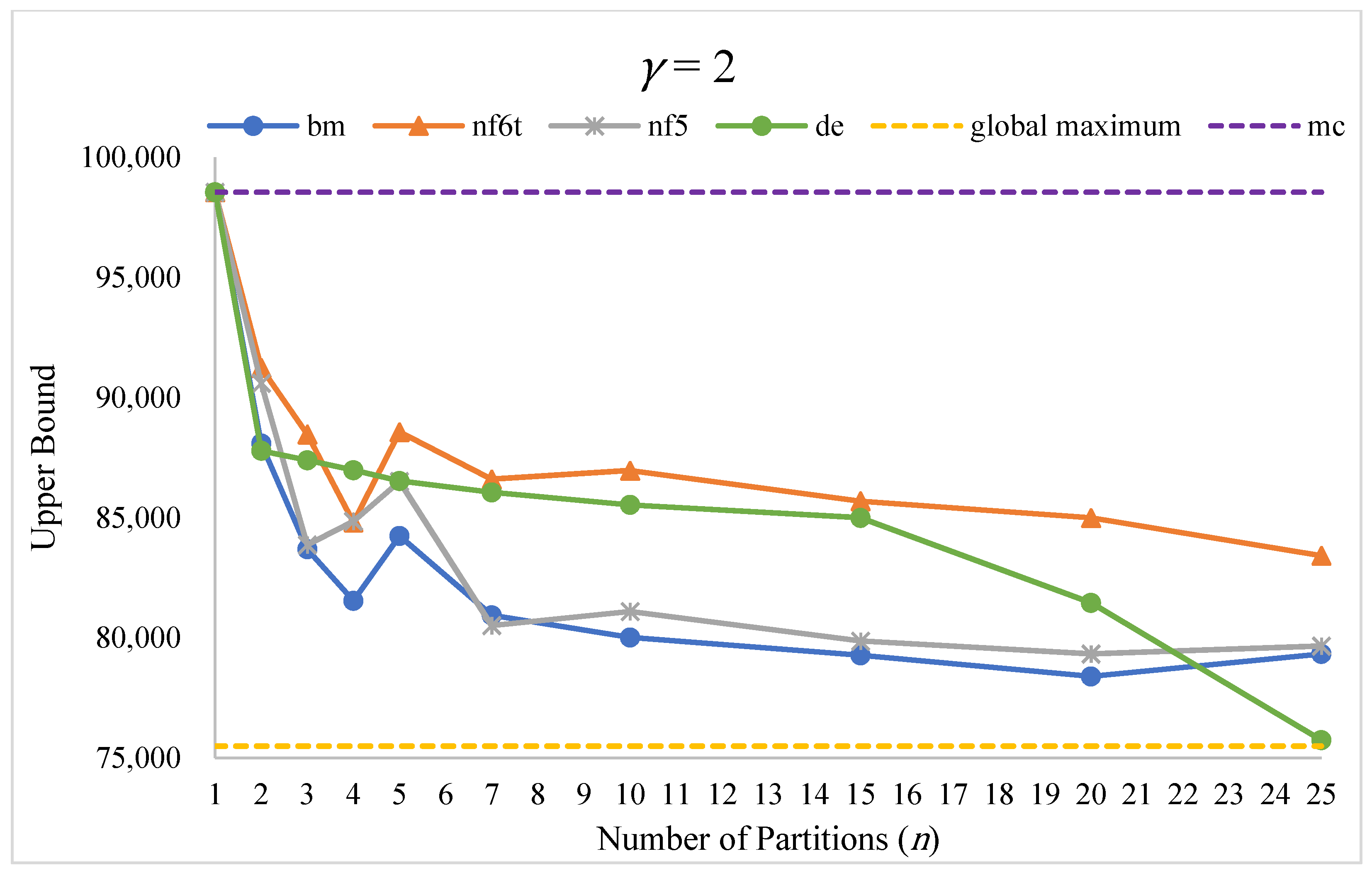
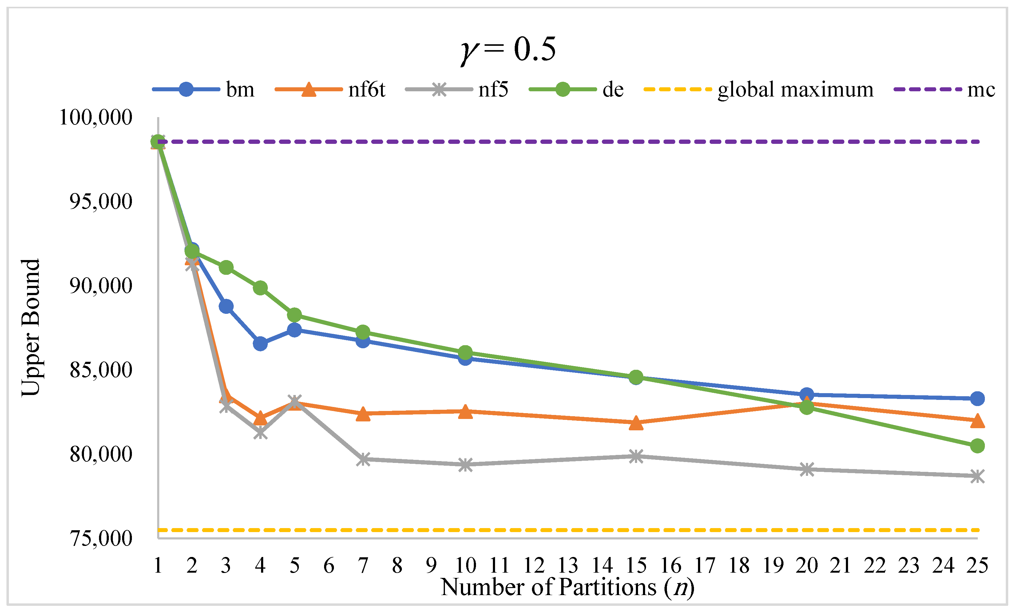
3.2. Computational Results

The original refinery planning model was solved using BARON and ANTIGONE, in which both reported the same ε-global optimal value of US$75,494 for the objective function (profit maximization). The relaxed models were reformulated as MILP and solved to obtain an upper bound of US$98,547 for the maximization objective function.
Each of the relaxed models was solved by varying the associated number of partitions n (for n = 1, 2, 3, 4, 5, 7, 10, 15, 20, 25) and partition size γ (for γ = 0.25, 0.5, 1, 1.5, 2, 3, 4) with the model performance shown in Figure 4, Figure 5, Figure 6, Figure 7, Figure 8, Figure 9 and Figure 10. We observed that as γ decreased to values less than unity (in which γ = 1 corresponds to uniform partitioning), the magnitude of the difference between an upper bound (given by relaxed model solution) and a global optimum generally increased in the order of nf5 < nf6t < de < bm (see Figure 4, Figure 5 and Figure 6). On the contrary, as γ increased to values greater than unity, the difference in magnitude between an upper bound and a global optimum generally increased in the order of bm < de < nf5 < nf6t (see Figure 7, Figure 8, Figure 9 and Figure 10).
The difference in magnitude between an upper bound and a global optimum can denote the tightness of a relaxation scheme: A smaller difference indicates greater tightness and vice versa. A convexified model using nf5 employed more constraints and an extra continuous variable that resulted in a tighter relaxation than nf6t, but at the expense of a larger size, which is consistent with the results reported by Gounaris et al. [39], while that of bm and de varied with respect to γ . In terms of the relaxed model sizes, which were in the order of bm < de < nf6t < nf5, a larger relaxation size (i.e., with more constraints) typically resulted in a tighter relaxation. We also found that relaxation tightness is subject to the partitioning levels (n) and their sizes ( γ ). All of the relaxed models were solved within fractions of a second. The CPU times for the relaxation schemes are shown in Figure 11 as a function of the number of partitions in which a uniform partition size is considered as a representative case. The average values of CPU times were 0.144, 0.170, 0.180, and 0.216 for the bm, de, nf6t, and nf5 schemes, respectively, that increased with the number of partitions. The CPU time was highest for nf5 and lowest for bm (as consistent with their relative sizes). Overall, our findings corroborate that of [39], which reported CPU times for numerous benchmark problems and concluded that relaxation tightness reduces optimality gap rapidly but increases solution time due to the resulting larger model sizes.
We defined a convergence indicator (CI) in Equation (40) for a resulting relaxation model that measures the distance traversed by a relaxed solution toward attaining a global optimal solution:
CI = Upper   Bound | n = 1 Upper   Bound | n > 1 , n < N Upper   Bound | n = 1 Upper   Bound | n = N × 100    
At a certain partition level, a higher CI value means a lower separation between the relaxed solution and the ε-global optimum. This indicator was evaluated at a certain partition level n with respect to a corresponding upper bound (for n = 1) and a lower bound (for n = N), as tabulated in Table 4 for each relaxation scheme. For 1 n 10 , average CI values (of 0.92, 0.87, 0.90, and 0.72) were found for each of the five schemes (respectively), as also shown by the slope (steepness) of the curves in Figure 5, Figure 6, Figure 7, Figure 8, Figure 9, Figure 10 and Figure 11. Low CI values indicate the schemes that require more partitions to converge. For n 10 , lower average values of 0.08, 0.13, 0.10, and 0.28 were found for each scheme (respectively). We observed a limit on the number of partitions that exhibited a certain relaxation tightness, beyond which a very small increase in tightness or performance improvement was obtained, despite the increasing model size and computational load.
To investigate the performance of uniform and non-uniform partition sizes, we determined the relative difference or deviation of a relaxed solution from an ε-global optimal solution for each value of γ and n, as tabulated in Table 5. Uniform partitioning ( γ = 1 ) provided a relatively lower deviation compared to non-uniform partition sizes, thereby indicating better relaxation quality for the former in employing a piecewise linear relaxation scheme. This observation is again consistent with Gounaris et al. [37], thus asserting the advantage of uniform partitioning in reducing the optimality gap (i.e., between the nonconvex original objective function and that of the relaxed convex objective function for each partition).
Piecewise linear relaxations provide an upper bound (lower bound) on the objective function value for a maximization (minimization) problem. By applying several relaxation schemes for a representative refinery planning problem, our computational results show that the nf5 scheme performs well for uniform partition sizes and can be suitably incorporated as part of a global optimization procedure, whereas non-uniform partitioning works better with the bm scheme, particularly for a larger number of partitions.

4. Concluding Remarks

In this work, we applied piecewise linear relaxation schemes to convexify bilinear terms in a refinery planning NLP model and studied the resulting performance by varying the number and size of the partitions. We introduced a new relaxation scheme based on eigenvector decomposition that was shown to be able to provide good relaxation results, especially for non-uniform partition sizes. As alternatives to conventional measures (e.g., computational time or optimality gap, which are more applicable to large-scale industrial-size problems), we considered certain indicators to compare the schemes in terms of convergence and partitioning behavior. Our study encountered a limit on the number of partitions that contributed to relaxation tightness, which does not necessarily correspond to a large number of partitions. We also found that the relationship between a relaxed formulation size and its tightness significantly depends on the number and size (uniform/non-uniform) of the partitions. Furthermore, the computational results showed a better relaxation quality by using uniform partition sizes. These results are largely consistent with the literature.

Supplementary Materials

The following are available online at https://www.mdpi.com/article/10.3390/pr9091624/s1. The mathematical formulation of the refinery planning model is available as a Supporting Material (Equations (A1)–(A400)).

Author Contributions

Conceptualization, C.S.K.; methodology, C.S.K. and Z.A.R.; software, C.S.K.; validation, C.S.K. and Z.A.R.; formal analysis, C.S.K. and Z.A.R.; investigation, C.S.K. and Z.A.R.; resources, C.S.K. and H.Z.; data curation, C.S.K. and Z.A.R.; writing—original draft preparation, C.S.K. and Z.A.R.; writing—review and editing, C.S.K., Z.A.R. and H.Z.; visualization, C.S.K. and Z.A.R.; supervision, C.S.K. and H.Z.; project administration, C.S.K. and H.Z.; funding acquisition, C.S.K. and H.Z. All authors have read and agreed to the published version of the manuscript.

Funding

This research was funded by The Murata Science Foundation 2020 Cycle 1 (Project No.: 015ME0-184) and Universiti Teknologi PETRONAS Graduate Assistantship Scheme, grant number 20000015 (ID for Zaid Ashraf Rana).

Acknowledgments

The authors would like to thank The Murata Science Foundation 2020 Cycle 1 (Project No.: 015ME0-184) and Universiti Teknologi PETRONAS for the funding and facility provided for this work.

Conflicts of Interest

The authors declare no conflict of interest.

Nomenclature

Sets and indices
U Set of process unit u
P Set of CDU fraction p
N Set of gridpoints for segment n
Parameters
γ Segment size (i.e., length)
MBig-M parameter
k n ,   p Gridpoint for segment n
qnLength of segment n
Continuous variables
L u Load of process unit u
W p Weight transfer ratio of fraction p (for CDU)
d W Deviation of partitioned variables in bilinear term from lower bound
d U ,   d V Auxiliary variable for relaxation
ω u , p Variable for reformulation to replace bilinear terms
Binary variables
λ Disjunction in bm scheme
θ   Disjunction in nf5 and nf6t formulations

References

  1. Aspen Technology. Aspen PIMS and Aspen PIMS-AO. 2013. Available online: http://www.aspentech.com/brochures/aspen_pims_ao.pdf (accessed on 15 August 2013).
  2. Honeywell. Symphonite RPMS (Refining and Petrochemical Modeling System); Honeywell: Toronto, ON, Canada, 2020. [Google Scholar]
  3. Haverly Systems. GRTMPS. 2012. Available online: http://www.haverly.com/main-products/13-products/9-grtmps (accessed on 9 August 2012).
  4. Barsamian, A. Fundamentals of Supply Chain Management for Refining. In IBC Asia Oil & Gas SCM Conference Proceedings; 2001. [Google Scholar]
  5. Andrade, T.; Ribas, G.; Oliveira, F. A Strategy Based on Convex Relaxation for Solving the Oil Refinery Operations Planning Problem. Ind. Eng. Chem. Res. 2016, 55, 144–155. [Google Scholar] [CrossRef]
  6. Rigby, B.; Lasdon, L.S.; Waren, A.D. The Evolution of Texaco’s Blending Systems: From OMEGA to StarBlend. Interfaces 1995, 25, 64–83. [Google Scholar] [CrossRef]
  7. Moro, L.F.L.; Zanin, A.C.; Pinto, J.M. A planning model for refinery diesel production. Comput. Chem. Eng. 1998, 22, S1039–S1042. [Google Scholar] [CrossRef]
  8. Steinschorn, D.; Hofferl, F. Refinery Scheduling Using Mixed Integer LP and Dynamic Recursion. In National Petroleum Refiners Association—Publications—All Series; National Petroleum Refiners Association: Houston, TX, USA, 1997. [Google Scholar]
  9. Khor, C.S.; Varvarezos, D. Petroleum refinery optimization. Optim. Eng. 2016, 18, 943–989. [Google Scholar] [CrossRef]
  10. Khor, C.S.; Elkamel, A. Roles of Computers in Petroleum Refineries. In Handbook of Petroleum Refining and Natural Gas Processing; Riazi, M.R., Eser, S., Diez, J.L.P., Agrawal, S.S., Eds.; ASTM International: Conshohocken, PA, USA, 2013; pp. 685–700. [Google Scholar]
  11. Watkins, R.N. Petroleum Refinery Distillation; Houston (Tex.), Book Division; Gulf Publishing Company: London, UK; Paris, France, 1979. [Google Scholar]
  12. Hasan, M.M.F.; Karimi, I. Exergy analysis of multi-stage crude distillation units. Front. Chem. Sci. Eng. 2013, 7, 437–446. [Google Scholar]
  13. Li, J.; Misener, R.; Floudas, C.A. Scheduling of crude oil operations under demand uncertainty: A robust optimization framework coupled with global optimization. AIChE J. 2012, 58, 2373–2396. [Google Scholar] [CrossRef]
  14. Li, J.; Misener, R.; Floudas, C.A. Continuous-time modeling and global optimization approach for scheduling of crude oil operations. AIChE J. 2012, 58, 205–226. [Google Scholar] [CrossRef]
  15. Geddes, R.L. A general index of fractional distillation power for hydrocarbon mixtures. AIChE J. 1958, 4, 389–392. [Google Scholar] [CrossRef]
  16. Menezes, B.C.; Kelly, J.D.; Grossmann, I.E. Improved Swing-Cut Modeling for Planning and Scheduling of Oil-Refinery Distillation Units. Ind. Eng. Chem. Res. 2013, 52, 18324–18333. [Google Scholar] [CrossRef]
  17. Lee, S.; Grossmann, I.E. Cutpoint Temperature Surrogate Modeling for Distillation Yields and Properties. Ind. Eng. Chem. Res. 2020, 59, 18616–18628. [Google Scholar]
  18. Brooks, R.; Walsem, F.D.; Drury, J. Choosing cutpoints to optimize product yields. Hydrocarb. Process. 1999, 78, 53–60. [Google Scholar]
  19. Uribe-Rodriguez, A.; Castro, P.M.; Gonzalo, G.-G.; Chachuat, B. Two-stage stochastic programming with fixed recourse via scenario planning with economic and operational risk management for petroleum refinery planning under uncertainty. Chem. Eng. Process. Process Intensif. 2008, 47, 1744–1764. [Google Scholar]
  20. Pinto, J.M.; Joly, M.; Moro, L.F.L. Planning and scheduling models for refinery operations. Comput. Chem. Eng. 2000, 24, 2259–2276. [Google Scholar] [CrossRef]
  21. Alattas, A.M.; Grossmann, I.E.; Palou-Rivera, I. Integration of Nonlinear Crude Distillation Unit Models in Refinery Planning Optimization. Ind. Eng. Chem. Res. 2011, 50, 6860–6870. [Google Scholar] [CrossRef]
  22. Trierwiler, Advances in Crude Oil LP Modeling; National Petrochemical & Refiners Association: Houston, TX, USA, 2001.
  23. Salhi, A.; Horst, R.; Tuy, H. A nonlinear programming model for refinery planning and optimisation with rigorous process models and product quality specifications. Int. J. Oil Gas Coal Technol. 2008, 1, 283–307. [Google Scholar]
  24. Williams, H.P.; Nemhauser, G.L.; Wolsey, L.A. Overall integration of the management of H2 and CO2 within refinery planning using rigorous process models. Chem. Eng. Commun. 2013, 200, 139–161. [Google Scholar]
  25. Zhang, J.; Zhu, X.; Towler, G. A Level-by-Level Debottlenecking Approach in Refinery Operation. Ind. Eng. Chem. Res. Ind. Eng. Chem. Res. 2001, 40, 1528–1540. [Google Scholar] [CrossRef]
  26. Li, W.; Hui, C.-W.; Li, A. Integrating CDU, FCC and product blending models into refinery planning. Comput. Chem. Eng. 2005, 29, 2010–2028. [Google Scholar] [CrossRef]
  27. Menezes, B.C.; Moro, L.F.; Lin, W.O.; Medronho, R.A.; Pessoa, F.L. Nonlinear Production Planning of Oil-Refinery Units for the Future Fuel Market in Brazil: Process Design Scenario-Based Model. Ind. Eng. Chem. Res. 2014, 53, 4352–4365. [Google Scholar] [CrossRef]
  28. Guerra, O.J.; Le Roux, G.A.C. Improvements in Petroleum Refinery Planning: 1. Formulation of Process Models. Ind. Eng. Chem. Res. 2011, 50, 13403–13418. [Google Scholar] [CrossRef]
  29. Guerra, O.J.; Le Roux, G.A.C. Improvements in Petroleum Refinery Planning: 2. Case Studies. Ind. Eng. Chem. Res. 2011, 50, 13419–13426. [Google Scholar] [CrossRef]
  30. Li, J.; Xiao, X.; Boukouvala, F.; Floudas, C.A.; Zhao, B.; Du, G.; Su, X.; Liu, H. Data-Driven Mathematical Modeling and Global Optimization Framework for Entire Petrochemical Planning Operations. AIChE J. 2016, 62, 3020–3040. [Google Scholar] [CrossRef]
  31. Alattas, A.M.; Grossmann, I.E.; Palou-Rivera, I. Refinery Production Planning: Multiperiod MINLP with Nonlinear CDU Model. Ind. Eng. Chem. Res. 2012, 51, 12852–12861. [Google Scholar] [CrossRef] [Green Version]
  32. Castillo Castillo, P.; Castro, P.M.; Mahalec, V. Global Optimization Algorithm for Large-Scale Refinery Planning Models with Bilinear Terms. Ind. Eng. Chem. Res. 2017, 56, 530–548. [Google Scholar] [CrossRef]
  33. McCormick, G.P. Computability of global solutions to factorable nonconvex programs: Part I—Convex underestimating problems. Math. Program. 1976, 10, 147–175. [Google Scholar] [CrossRef]
  34. Al-Khayyal, F.A.; Falk, J.E. Jointly constrained biconvex programming. Math. Oper. Res. 1983, 8, 273–286. [Google Scholar] [CrossRef]
  35. Misener, R.; Floudas, C.A. ANTIGONE: Algorithms for coNTinuous/Integer Global Optimization of Nonlinear Equations. J. Glob. Optim. 2014, 59, 503–526. [Google Scholar] [CrossRef]
  36. Meyer, C.A.; Floudas, C.A. Global optimization of a combinatorially complex generalized pooling problem. AIChE J. 2006, 52, 1027–1037. [Google Scholar] [CrossRef]
  37. Karuppiah, R.; Grossmann, I.E. Global optimization for the synthesis of integrated water systems in chemical processes. Comput. Chem. Eng. 2006, 30, 650–673. [Google Scholar] [CrossRef] [Green Version]
  38. Wicaksono, D.S.; Karimi, I.A. Piecewise MILP under- and overestimators for global optimization of bilinear programs. AIChE J. 2008, 54, 991–1008. [Google Scholar] [CrossRef]
  39. Gounaris, C.E.; Misener, R.; Floudas, C.A. Computational Comparison of Piecewise−Linear Relaxations for Pooling Problems. Ind. Eng. Chem. Res. 2009, 48, 5742–5766. [Google Scholar] [CrossRef]
  40. Hasan, M.M.F.; Karimi, I.A. Piecewise linear relaxation of bilinear programs using bivariate partitioning. AIChE J. 2009, 56, 1880–1893. [Google Scholar] [CrossRef]
  41. Misener, R.; Floudas, C.A. Advances for the pooling problem: Modeling, global optimization, and computational studies. Appl. Comput. Math. 2009, 8, 3–22. [Google Scholar]
  42. Nagarajan, H.; Lu, M.; Wang, S.; Bent, R.; Sundar, K. An adaptive, multivariate partitioning algorithm for global optimization of nonconvex programs. J. Glob. Optim. 2019, 74, 639–675. [Google Scholar] [CrossRef] [Green Version]
  43. Tawarmalani, M.; Ahmed, S.; Sahinidis, N.V. Global optimization of 0–1 hyperbolic programs. J. Glob. Optim. 2002, 24, 385–416. [Google Scholar] [CrossRef]
  44. Tawarmalani, M.; Sahinidis, N.V. Convexification and Global Optimization in Continuous and Mixed-Integer Nonlinear Programming: Theory, Algorithms, Software, and Applications. Nonconvex Optimization and Its Applications; Kluwer Academic Publishers: Dordrecht, The Netherlands, 2002; Volume 65, p. 504. [Google Scholar]
  45. Grossmann, I.E.; Lee, S. Global optimization of nonlinear generalized disjunctive programming with bilinear equality constraints: Applications to process networks. Comput. Chem. Eng. 2003, 27, 1557–1575. [Google Scholar]
  46. Uribe-Rodriguez, A.; Castro, P.M.; Gonzalo, G.G.; Chachuat, B. Global optimization of large-scale MIQCQPs via cluster decomposition: Application to short-term planning of an integrated refinery-petrochemical complex. Comput. Chem. Eng. 2020, 140, 106883. [Google Scholar] [CrossRef]
  47. Yang, H.; Bernal, D.E.; Franzoi, R.E.; Engineer, F.G.; Kwon, K.; Lee, S.; Grossmann, I.E. Integration of crude-oil scheduling and refinery planning by Lagrangean Decomposition. Comput. Chem. Eng. 2020, 138, 106812. [Google Scholar] [CrossRef]
  48. Sergeyev, Y.D. Global one-dimensional optimization using smooth auxiliary functions. Math. Program. 1998, 81, 127–146. [Google Scholar] [CrossRef]
  49. Sergeyev, Y.D. On convergence of “Divide the Best” global optimization algorithms. Optimization 1998, 44, 303–325. [Google Scholar] [CrossRef]
  50. Horst, R.; Tuy, H. Global Optimization: Deterministic Approaches, 3rd ed.; Springer: Berlin/Heidelberg, Germany, 1996. [Google Scholar]
  51. Nemhauser, G.; Wolsey, L. Integer and Combinatorial Optimization; Wiley: New York, NY, USA, 1988. [Google Scholar]
  52. Tawarmalani, M.; Sahinidis, N.V. Global optimization of mixed-integer nonlinear programs: A theoretical and computational study. Math. Program. 2004, 99, 563–591. [Google Scholar] [CrossRef]
  53. Tawarmalani, M.; Sahinidis, N.V. A polyhedral branch-and-cut approach to global optimization. Math. Program. 2005, 103, 225–249. [Google Scholar] [CrossRef]
  54. Sahinidis, N.V.; Tawarmalani, M. BARON 7.2.5: Global Optimization of Mixed-Integer Nonlinear Programs, User’s Manual. 2005. Available online: http://www.gams.com/dd/docs/solvers/baron.pdf (accessed on 1 July 2021).
  55. Zamora, J.M.; Grossmann, I.E. Continuous global optimization of structured process systems models. Comput. Chem. Eng. 1998, 22, 1749–1770. [Google Scholar] [CrossRef]
  56. Misener, R.; Floudas, C. GloMIQO: Global mixed-integer quadratic optimizer. J. Glob. Optim. 2013, 57, 3–50. [Google Scholar] [CrossRef] [Green Version]
  57. Neumaier, A. Complete search in continuous global optimization and constraint satisfaction. Acta Numer. 2004, 13, 271–369. [Google Scholar] [CrossRef] [Green Version]
  58. Smith, E.M.B.; Pantelides, C.C. A symbolic reformulation/spatial branch-and-bound algorithm for the global optimisation of nonconvex MINLPs. Comput. Chem. Eng. 1999, 23, 457–478. [Google Scholar] [CrossRef]
  59. Faria, D.C.; Bagajewicz, M.J. Global Optimization of Water Management Problems Using Linear Relaxation and Bound Contraction Methods. Ind. Eng. Chem. Res. 2011, 50, 3738–3753. [Google Scholar] [CrossRef]
  60. Faria, D.C.; Bagajewicz, M.J. Novel bound contraction procedure for global optimization of bilinear MINLP problems with applications to water management problems. Comput. Chem. Eng. 2011, 35, 446–455. [Google Scholar] [CrossRef]
  61. Faria, D.C.; Bagajewicz, M.J. A new approach for global optimization of a class of MINLP problems with applications to water management and pooling problems. AIChE J. 2012, 58, 2320–2335. [Google Scholar] [CrossRef]
  62. Faria, D.C.; Bagajewicz, M.J. Global optimization based on subspaces elimination: Applications to generalized pooling and water management problems. AIChE J. 2012, 58, 2336–2345. [Google Scholar] [CrossRef]
  63. Rote, G. The convergence rate of the sandwich algorithm for approximating convex functions. Computing 1992, 48, 337–361. [Google Scholar] [CrossRef]
Figure 1. Modeling methods for petroleum refinery distillation cutpoints (mainly for CDUs).
Processes 09 01624 g001
Figure 2. Flowsheet configuration for the refinery planning model (NLP).
Processes 09 01624 g002
Figure 3. Procedure for investigating the performance of piecewise linear relaxation schemes on a nonconvex bilinear refinery planning NLP model.
Processes 09 01624 g003
Figure 4. Convergence-indicating curves of the bm, de, nf5, and nf6t relaxation schemes for γ = 0.25.
Processes 09 01624 g004
Figure 5. Convergence-indicating curves of the bm, de, nf5, and nf6t relaxation schemes for γ = 0.5.
Processes 09 01624 g005
Figure 6. Convergence-indicating curves of the bm, de, nf5, and nf6t relaxation schemes for γ = 1.
Processes 09 01624 g006
Figure 7. Convergence-indicating curves of the bm, de, nf5, and nf6t relaxation schemes for γ = 1.5.
Processes 09 01624 g007
Figure 8. Convergence-indicating curves of the bm, de, nf5, and nf6t relaxation schemes for γ = 2.
Processes 09 01624 g008
Figure 9. Convergence-indicating curves of the bm, de, nf5, and nf6t relaxation schemes for γ = 3.
Processes 09 01624 g009
Figure 10. Convergence-indicating curves of the bm, de, nf5, and nf6t relaxation schemes for γ = 4.
Processes 09 01624 g010
Figure 11. CPU times of the relaxation schemes.
Processes 09 01624 g011
Table 1. Methods to model the refinery distillation yields of crude oils.
MethodRelation TypeFeatureApplication
Fixed yieldLinearSimple; amenable to large-scale models (especially LP); can cater for different operating modesSimulation [18], planning optimization (LP [18], NLP [7,19], MINLP [20]), and scheduling optimization (MILP [8])
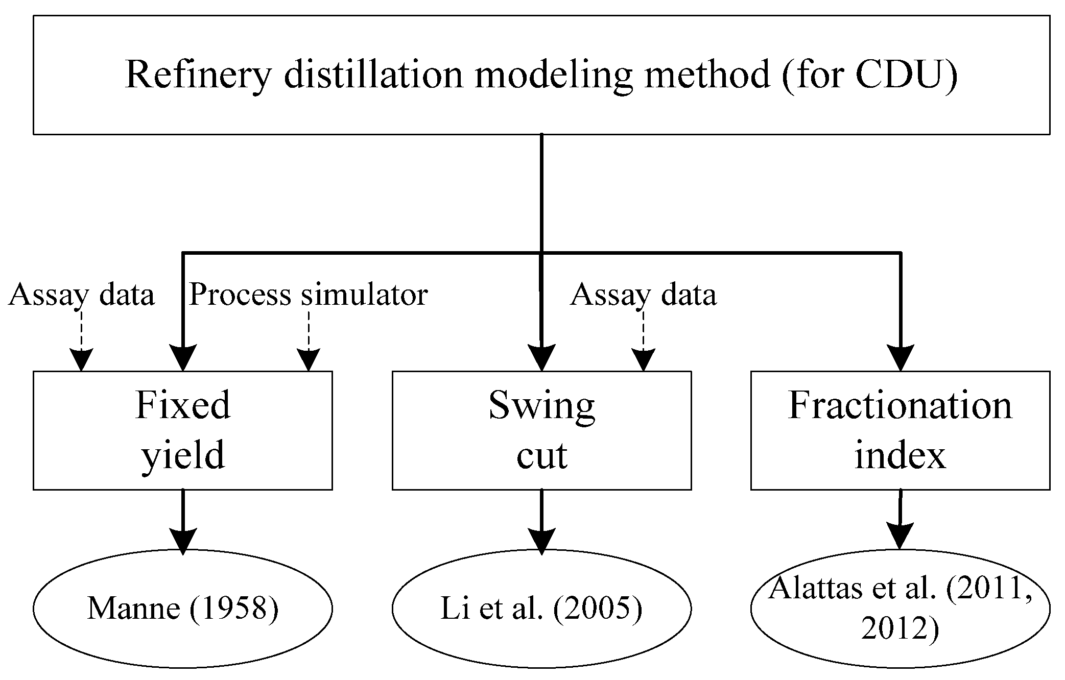
Swing cutLinear or nonlinearMore accurate than fixed yield; can represent multiple operating modes [21]Planning optimization (LP [22], MILP, NLP [16,23,24,25,26,27,28,29], and MINLP [30])
Fractionation indexNonlinearHigh accuracy (considers relative volatility and phase equilibrium)Planning optimization (NLP [21] and MINLP) [31,32]
Table 2. Model size and computational statistics for refinery planning NLP model.
Computing platformGAMS 30.3.0/CPLEX 12; 1.9 GHz (speed, Intel Core i3); 8192 MB (RAM)
No. of continuous variables49
No. of nonlinear variables42
No. of constraints61
No. of nonconvex terms21 (bilinear)
Table 3. Bilinear terms in the refinery planning NLP model.
Bilinear TermCount
L u W p 5
L u Y f 4
C o n v × C o n v = ( C o n v ) 2 4
M W p × M W p = M W p 2 4
P r j , p F p , g i p r o d 4
Total21
Table 4. Convergence indicator of the bm, de, nf5, and nf6t relaxation schemes with partition size variation.
γ Convergence Indicator
for   1 n 10
Convergence Indicator (%)
for   n 10
bmnf6tnf5debmnf6tnf5de
0.250.890.950.900.710.110.500.100.29
0.50.840.970.970.690.160.030.030.31
10.920.900.890.680.080.100.110.32
1.50.930.960.850.590.070.040.150.41
20.970.770.920.560.030.230.080.44
30.950.850.990.890.050.150.010.11
40.910.700.800.910.090.300.200.09
Table 5. Relative differences of the bm, de, nf5, and nf6t relaxation schemes from an ε-global optimal solution with partition size variation.
γ Relative Difference (%)
bmnf6tnf5de
0.250.6420.4930.4650.530
0.50.4500.2980.2590.458
10.3200.2550.2510.472
1.50.2900.4050.2950.395
20.2670.4800.3180.375
30.3600.5660.4000.341
40.4900.6520.4550.250
Publisher’s Note: MDPI stays neutral with regard to jurisdictional claims in published maps and institutional affiliations.

