Review of Soft Sensors in Anaerobic Digestion Process

Abstract

Anaerobic digestion is associated with various crucial variables, such as biogas yield, chemical oxygen demand, and volatile fatty acid concentration. Real-time monitoring of these variables can not only reflect the process of anaerobic digestion directly but also accelerate the efficiency of resource conversion and improve the stability of the reaction process. However, the current real-time monitoring equipment on the market cannot be widely used in the industrial production process due to its defects such as expensive equipment, low accuracy, and lagging analysis. Therefore, it is essential to conduct soft sensor modeling for unmeasurable variables and use auxiliary variables to realize real-time monitoring, optimization, and control of the an-aerobic digestion process. In this paper, the basic principle and process flow of anaerobic digestion are first briefly introduced. Subsequently, the development history of the traditional soft sensor is systematically reviewed, the latest development of soft sensors was detailed, and the obstacles of the soft sensor in the industrial production process are discussed. Finally, the future development trend of deep learning in soft sensors is deeply discussed, and future research directions are provided.

1. Introduction

Anaerobic digestion is a highly complex biochemical reactions process, with characteristics such as multi-factor influence, dynamic change, and complex nonlinearity [1]. Anaerobic digestion can not only treat organic pollutants but also produce clean energy [2]. Therefore, anaerobic digestion technology has broad development space in the treatment of wastewater and organic solid waste [3] and is one of the practical ways to solve energy and environmental problems. However, anaerobic microorganisms of the anaerobic digestion process are intensely sensitive to changes in the digestion environment, and methanogens have extremely strict requirements on the external environment [3]. The unexpected changes in the external environment have an impact on the hydrolysis, acidification, and methanation processes of anaerobic digestion [4,5]. This will cause numerous volatile fatty acids (VFA) to accumulate in the reactor, inhibit the progress of methanation, and even result the failure of the anaerobic reactor operation [6,7,8]. Therefore, a more advanced online measurement system must be used to fully monitor the anaerobic digestion process in real-time to ensure that the anaerobic digestion process is stable and efficient while obtaining a higher biogas yield [9].

In terms of anaerobic digestion process variables monitoring, there is mature and reliable online monitoring equipment for temperature, pressure, flow rate, gas composition, and other variables [10,11]. However, there are still many key variables that cannot be directly measured, or the measurement equipment is expensive [12], such as biogas yield, chemical oxygen demand (COD), and VFA concentration. Online monitoring equipment for these variables cannot be widely used in industrial production due to factors such as expensive equipment, low accuracy, and lagging analysis [13,14,15,16]. Consequently, the soft sensor using online measurable auxiliary variables to estimate the unmeasurable variables in real-time has been broadly used in the anaerobic digestion process [17,18]. The soft sensor is developed based on the inference control theory proposed by Brosilow [19], suggesting that the mathematical relationship between auxiliary variables and target variables is established under certain optimal criteria, and the selection of auxiliary variables should be measurable and easy-to-obtain [20]. Real-time monitoring of target variables is achieved through software [21]. Since the soft sensor has the advantages of fast response, low cost, easy implementation, and simple maintenance [22], it has been widely used in monitoring, optimization, and control of engineering [23]. Soft-sensor technology is broadly based on two modelling approaches: those derived mechanistically and those that are data-driven [24]. Specifically, mechanism models can be classified into common mechanism models and state estimation and system identification based on mechanism models [25]. Data-driven models can be divided into statistical machine learning models and deep learning models.

In this paper, the basic principle and process flow of anaerobic digestion are first briefly introduced. Subsequently, the soft sensors in the anaerobic digestion process are compared and analyzed, the development process of traditional soft sensors is systematically reviewed, and the defects of traditional soft sensors are presented. Next, the latest development of soft sensors is detailed, including the application of deep learning in the anaerobic digestion process. Moreover, the obstacles encountered by soft sensors in industrial production are further discussed. Finally, the future development trend of deep learning in soft sensors is deeply analyzed, and a summary and outlook are drawn.

2. Anaerobic Digestion Process

2.1. Basic Principles of Anaerobic Digestion

According to the four-stage theory of anaerobic digestion proposed by Zeikus, the anaerobic digestion process can be divided into four stages: hydrolysis, acidification, acetic acidification, and methanation [26]. In the hydrolysis stage, the hydrolase hydrolyzes macromolecular organics (such as protein, fat, and cellulose) into small molecular organics (such as glucose, amino acids, and long-chain fatty acids) for subsequent reactions [26]. After the initial hydrolysis, small-molecule organic substances (such as glucose and amino acids) will be further decomposed by acid-producing bacteria to produce acidified products mainly short-chain fatty acids and secondary metabolites (such as hydrogen and carbon dioxide) [27]. In the acetification stage, acetogens convert the organic acids and alcohols produced in the hydrolysis and acidification stages into acetic acid, generating carbon dioxide and hydrogen [28]. In the methanation stage, acetic acid, hydrogen, and carbon dioxide are converted into methane under the action of obligate anaerobic methanogens [29].

2.2. Process Parameters of Anaerobic Digestion

There are some essential process variables in the anaerobic digestion process, such as pH, alkalinity, temperature, VFA concentration, COD, and biogas yield. Real-time monitoring of the above variables can ensure the efficient and stable operation of the anaerobic digestion process. However, there is little widely used real-time monitoring equipment for VFA concentration, COD, and biogas yield.

• PH: The optimal pH range of different microorganisms is different. Methanogens are extremely sensitive to pH, and the optimal pH range is 6.5–7.2 [30]. The fermenting microorganisms produce acetic acid and butyric acid when the pH is low. Acetic acid and propionic acid are formed when the pH is higher than 8.0 [31]. Therefore, reasonable monitoring of pH can ensure the maximum biological activity of microorganisms.
• Alkalinity: Methanogens usually produce alkalinity in the form of carbon dioxide, ammonia, and bicarbonate, contributing to neutralizing VFA produced during anaerobic digestion [32]. Thus, real-time monitoring of alkalinity can improve the stability of the anaerobic digestion process when the concentration of carbon dioxide is stable.
• Temperature: Temperature has a crucial influence on the physical and chemical properties of anaerobic digestion and fermentation substrates. It affects the growth rate and metabolism of microorganisms, which in turn influences the population dynamics of the anaerobic digestion process [33]. When the temperature changes more than 1 °C/day, the biochemical activity of methanogens will be severely affected, causing the process to fail.
• VFA concentration: VFA concentration is an intermediate product of the anaerobic digestion process. Excessive accumulation of VFA can reduce the pH of the system and inhibit the activity of methanogens. The VFA concentration can reflect the current operating conditions of the system while being extremely sensitive to the incoming feed imbalance [34]. Hence, it is urgent to establish a soft sensor to predict the VFA concentration by monitoring the measurable and easy-to-obtain process variables in real-time.
• COD and biogas yield: COD is an imperative indicator to measure the organic content of the effluent from the anaerobic digestion process [35]. Biogas yield is a vital indicator to measure the efficiency of anaerobic digestion [36]. Real-time monitoring of COD and biogas yield can demonstrate the operating efficiency and stability of the anaerobic digestion process and contribute to achieving the real-time calibration and optimization of production conditions and control methods.

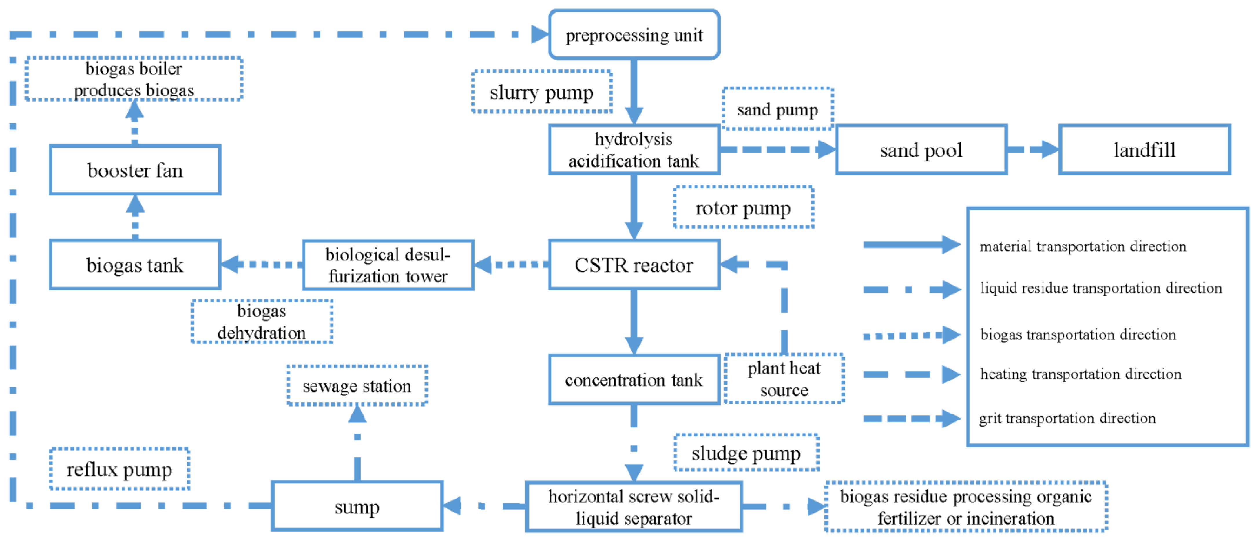
2.3. Anaerobic Digestion Process

In the industrial production process, anaerobic digestion processes are usually classified according to factors such as operating temperature, feeding method, and the number of reactors [37]. It can be divided into single-phase digestion and two-phase digestion based on the number of reactors [38]. The single-phase digestion process was widely used in the immature stage of the early anaerobic digestion theory due to its low price and simple operation. Single-phase digestion suggests that the hydrolysis, acidification, acetic acidification, and methanation processes of degrading macromolecular organics are all conducted in the same digestion tank, and the inhibition of any one step will affect the overall digestion efficiency [39]. With the development of the anaerobic digestion theory, researchers and technologists have developed a two-phase digestion process to avoid acid inhibition. Two-phase anaerobic digestion suggests the hydrolysis, acidification, and acetic acid stages are conducted in the acid production tank, while the methane production stage is performed in the methane production tank [40]. This method can effectively avoid mutual inhibition between the steps, improve the efficiency of anaerobic digestion, shorten the reaction time, and increase methane production [41].

According to the biodegradability of the input materials, different two-phase anaerobic digestion devices are generally selected [42]. When industrial wastewater is treated with low solid content, the acid production tank and the methane production tank usually adopt a continuous stirred tank reactor and an up-flow anaerobic sludge blanket, respectively [43]. When organic wastewater is treated with high solid content, both the acid production tank and the methane production tank use the up-flow solid reactor [44]. When organic sludge is processed with higher solid content, both the acid production tank and the methane production tank employ the continuous stirred tank reactor [45]. The specific process flow is described as follows [28]. First, the pretreated organic materials are fed into the hydrolysis acidification tank to perform the hydrolysis reaction of macromolecular organics and the acidification reaction of small molecular organics. Then, the acidified product is input into the methane-generating tank for methane production reaction. Since the stages of acid production and methane production are performed separately, it is ensured that acid-producing bacteria and methanogens are in optimal environmental conditions and can exert maximum activity. Moreover, the acid production process improves the biochemical properties of the material, and the acidified product provides a suitable substrate for methanogens. The two-phase anaerobic digestion process is illustrated in Figure 1.

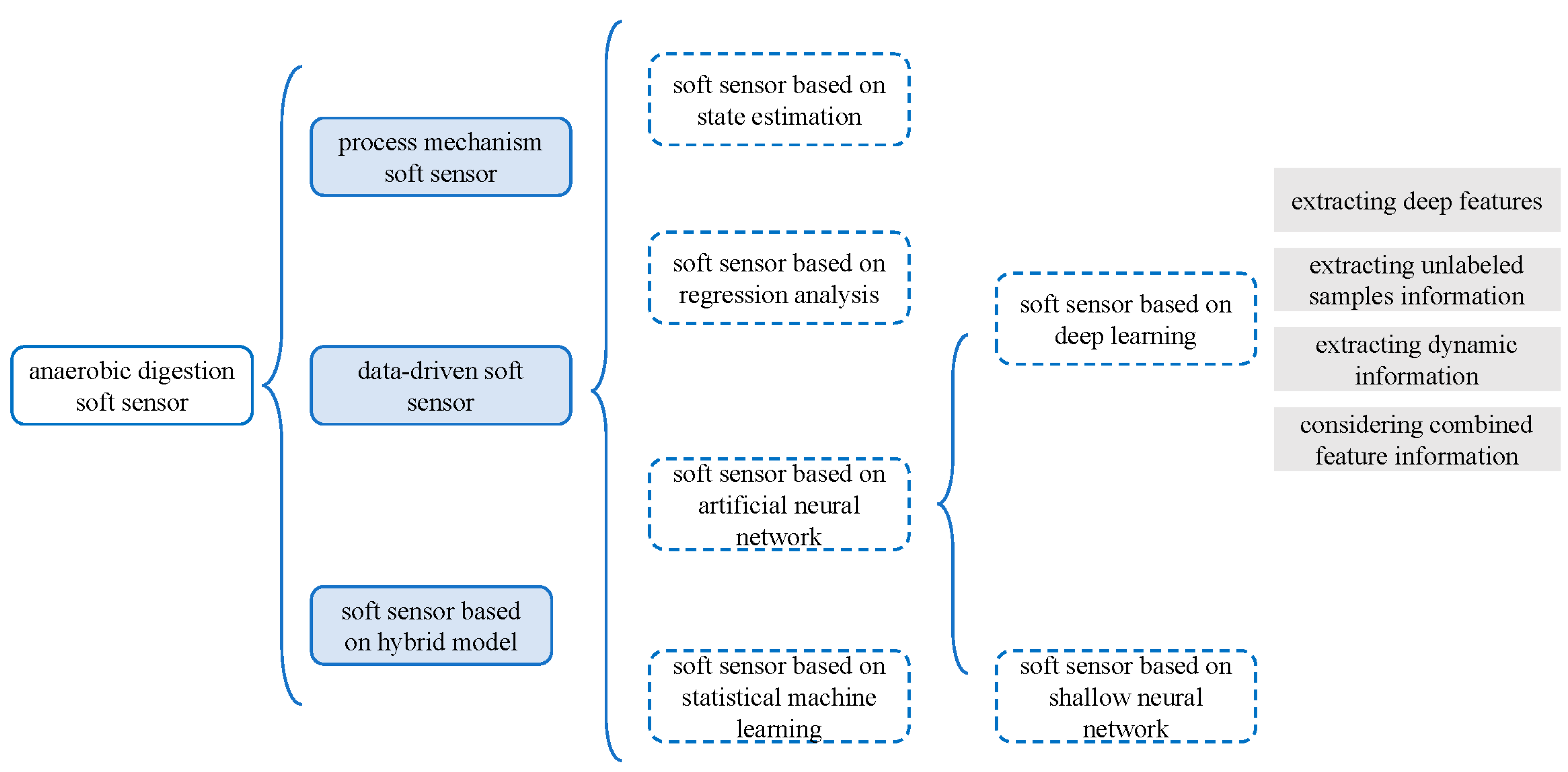
3. Development History of Anaerobic Digestion Soft Sensor

3.1. Soft Sensor Based on Process Mechanism

Mechanism modeling is to determine the mathematical relationship between the target variables and the auxiliary variables through the establishment of a balance equation based on a deep understanding of the process mechanism [23]. It has the advantages of high accuracy, strong interpretability, and clear industrial background. However, the biochemical reaction process of anaerobic digestion is extremely complicated, with strong nonlinearity and uncertainty, making it difficult to establish an accurate mechanism model [46,47]. Moreover, the biochemical reaction process is described by a large number of algebraic equations and differential equations. Therefore, there are defects such as large calculation amount and slow convergence, impeding it in meeting the requirements of real-time monitoring of target variables [48,49,50]. From another perspective, the mechanism model parameters of anaerobic digestion, such as Monod maximum specific absorption rate and the first-order decay rate in the kinetic parameters of the Anaerobic Digestion Model No.1 (ADM1), are mostly empirical values [51]. The determination of these parameters requires considerable experimental verifications, and the various indicators in the industrial production process will not be tested. Therefore, it is proposed to combine the mechanism model and the data-driven model to establish a hybrid model of anaerobic digestion [52,53]. The hybrid model fully takes advantage of the data-driven model that only pays attention to input and output and does not require a clear internal mechanism, contributing to a decrease in the difficulty of modeling the mechanism model. Moreover, the interpretability of the data-driven model is enhanced using the mechanism model. However, the prediction accuracy and generalization ability of the hybrid model need to be further improved.

3.2. Soft Sensor Based on State Estimation

In the soft sensor based on state estimation, the method of state observation and state estimation is adopted to obtain the predicted value of the state variable through auxiliary variables and then acquire the predicted value of the target variable [54,55]. With the development of anaerobic digestion soft sensors, various soft sensors based on state estimation have been proposed [56,57,58,59,60,61]. Among them, the nonlinear observer presented by Dochain under the improved anaerobic digestion model can estimate the VFA concentration online under different working conditions [62]. The improved anaerobic digestion model can be expressed as:

$$\{\begin{array}{c}\dot{x}=f\left(x,\mu \right)+\Delta f\\ y=Cx\end{array}$$

(1)

where $\Delta f$ denotes the uncertainty item related to unmodeled dynamics and load disturbance; x is the vector of dynamic states; f denotes the vector field; C = [0, 0, 1]; u and y denote the input and output of the model, respectively. For the improved anaerobic digestion model, the nonlinear observer can be expressed as:

$$\dot{\widehat{x}}=f\left(\widehat{x},\mu \right)+k_l\left(y-\widehat{y}\right)+k_{d}tanh\left[\gamma \left(y-\widehat{y}\right)\right]$$

(2)

where $\widehat{x}\in R^3$ represents the state estimation vector, $\widehat{y}$ indicates the predicted value of the output signal, and $k_l,k_d$ and $\gamma$ denote the observer gains. The estimated error of the model is presented in Formula (3).

$$\dot{e}=f\left(x,u\right)-f\left(\widehat{x},u\right)+\Delta f-k_{l}Ce-k_{d}tanh\left(\gamma Ce\right)$$

(3)

where $Ce=y-\widehat{y}$. This nonlinear observer overcomes the disadvantage of the poor performance of the local observer under non-set conditions and solves the problem that the progressive observer is very sensitive to unknown load disturbances [63]. Additionally, the author has verified the convergence of the observer through Lyapunov stability. Soft sensors based on state estimation can handle situations such as dynamic characteristic differences between the variables and system lag. However, state estimation mainly applies to mature models and models that can reflect the characteristics of the measured object after approximation. Moreover, an increase in the online estimation error would be caused by simplifying the system to reduce the difficulty of modeling, and the use of this method would be restricted by the anaerobic digestion model’s requirements for modeling accuracy [64,65,66,67].

3.3. Soft Sensor Based on Regression Analysis

The soft sensor of anaerobic digestion based on regression analysis majorly includes soft sensors based on multiple linear regression (MLR) and soft sensors based on partial least squares regression (PLSR).

MLR is able to establish a linear mapping between auxiliary variables and target variables through the least square method [68]. The soft sensor of anaerobic digestion based on MLR proposed by HU assumes the following linear relationship between auxiliary variables and biogas yield [69]:

$$\widehat{y}={\theta }_0+{\theta }_1{X}_1+{\theta }_2{X}_2+···+{\theta }_n{X}_n$$

(4)

where $X$ is the auxiliary variable, $\theta$ is the parameter to be calculated, and $\widehat{y}$ is the predicted value of biogas yield. The target parameter $\theta$ is solved by minimizing the error of the real biogas yield and the predicted biogas yield with the least squares method. However, the biochemical reaction process of anaerobic digestion is significantly nonlinear, and MLR cannot accurately describe the nonlinear process. Therefore, the anaerobic digestion soft sensor based on MLR has disadvantages such as low accuracy and susceptibility to external interference [70].

The anaerobic digestion soft sensor based on PLSR, which was proposed by Yang [1], can extract the principal components of auxiliary variables and target variables while maximizing the correlation between them [71]. The objective function of the soft sensor is expressed as

$$maxCov\left(t,y\right)=\sqrt{var\left(t\right)var\left(y\right)}corr\left(t,y\right)$$

(5)

where $t$ represents the main component of the auxiliary variable, and $y$ denotes the COD. The Lagrange multiplier l is introduced to solve the objective function.

$$l=p^T{x}^{T}y-\frac{\lambda }{2}\left(p^{T}p-1\right)$$

(6)

where $x$ and $p$ indicate the auxiliary variable and the weight coefficient, respectively. Subsequently, the linear fitting between the principal component and the COD is realized by the MLR algorithm. This model solves the problem of the collinearity of auxiliary variables in the anaerobic digestion process. Unfortunately, the process of dimensionality reduction may eliminate the secondary principal components that are beneficial to regression and retain irrelevant noise, affecting the accuracy of the model. Meanwhile, PLSR is a linear algorithm and is only suitable for linear and weakly nonlinear models. However, there is severe nonlinearity in the anaerobic digestion process, limiting the prediction accuracy and generalization ability of the model.

3.4. Soft Sensor Based on Artificial Neural Network

Artificial neural networks can establish a non-linear mapping relationship between auxiliary variables and target variables through network learning, including back propagation (BP) neural networks and radial basis function (RBF) neural networks.

The soft sensor based on the BP neural network for the anaerobic digestion process was proposed by researchers [72,73,74,75,76,77,78]. In this soft sensor, the gradient descent algorithm is used to update the network weight. Therefore, the soft sensor can approximate the continuous nonlinear function with arbitrary precision and solve the highly nonlinear and uncertain problems in the anaerobic digestion process [79,80]. However, it is prone to fall into a local optimal or over-fitting state, affecting the prediction accuracy and generalization ability of the soft sensor [81].

To handle the complication that the anaerobic digestion soft sensor based on the BP neural network is prone to fall into the local minimum, Yilmaz proposed a soft sensor based on the RBF neural network to predict COD [82]. The soft sensor based on the RBF neural network has the characteristics of global best approximation and strong nonlinear mapping ability. The loss function of the soft sensor is expressed as

$$Loss=\frac{1}{2}\Vert Y-{\widehat{Y}}^2\Vert +\frac{1}{2}\lambda \Vert D{\widehat{Y}\Vert }^2$$

(7)

where $Y$ and $\widehat{Y}$ denote the test and predicted values of COD, respectively; $\lambda$ represents the weighting factor of the regular term; $D$ indicates the linear differential operator. With the regularization term, the curvature of the approximation function can be controlled, and the problem that the model is prone to overfitting is addressed.

The soft sensor based on the neural network can better handle the problem of non-linearity in the anaerobic digestion process. However, the performance of soft sensors is dramatically affected by the network topology and hyperparameters in practical applications. Therefore, proper hyperparameters and network topology are selected through optimization algorithms such as genetic algorithm and particle swarm optimization algorithm to improve model prediction accuracy and generalization ability [83,84,85,86,87].

3.5. Soft Sensor Based on Statistical Machine Learning

The soft sensor based on support-vector regression (SVR) uses the kernel function to map auxiliary variables to the high-dimensional feature space and adopts linear algorithms to analyze the nonlinear characteristics of the samples in the high-dimensional feature space. The convex quadratic programming is solved by the structural risk minimization criterion, which also addresses the high-dimensional and small-sample problems that cannot be solved by artificial neural networks [88]. Given the small-sample problem caused by the difficulty of obtaining target variables in the anaerobic digestion process, Kazemi proposed the soft sensor based on SVR to predict the VFA concentration [89]. The loss function of the soft sensor is expressed as

$$Loss=\frac{1}{2}{{\displaystyle \sum }}_{i,j=1}^m\left(a_i-a_i^{*}\right)\left(a_j-a_j^{*}\right)k\left(x_i,x_j\right)+{{\displaystyle \sum }}_i^m{a}_i\left(\epsilon -y_i\right)+a_i^{*}\left(\epsilon +y_i\right)$$

(8)

The constraints are

$$s.t \{\begin{array}{c}{\displaystyle \sum }_{i=1}^m\left(a_i-a_i^{*}\right)=0\\ a_i,a_i^{*}\in \left[0,C\right]\end{array}$$

(9)

where $x$ is the auxiliary variable; $y$ indicates the VFA concentration; $a_i$ and $a_i^{*}$ are Lagrangian multipliers; $k(·)$ represents the kernel function; $\epsilon$ is the insensitivity coefficient.

Given the problem of high complexity in solving SVR models, a soft sensor based on least-squares support-vector regression (LS-SVR) was proposed by Liu to monitor the VFA concentration in the anaerobic digestion process in real-time [90]. In the soft sensor based on LS-SVR, the slack variable in the optimization objective is replaced with the quadratic square term of the training error.

$$Loss=\frac{1}{2}\Vert {w\Vert }^2+\frac{1}{2}\gamma {{\displaystyle \sum }}_{i=1}^m{\xi }_i^2$$

(10)

Then, the inequality constraints are replaced with the following equality constraints.

$$y_i\left(w{x}_i+b\right)=1-{\xi }_i$$

(11)

where $w$ and $b$ indicates the learnable parameter of the model, $\gamma$ denotes the regularization coefficient, and $\xi$ refers to the training error. Solving the problem of convex quadratic programming is transformed into solving a set of linear equations, reducing the complexity of the model. However, the simplified soft sensor is more sensitive to abnormal values in the anaerobic digestion process, weakening the robustness of the soft sensor. Therefore, optimization algorithms are used to select the appropriate kernel function and hyperparameters to improve the prediction accuracy and generalization ability of the model [91,92,93].

3.6. Practical Application of Soft Sensors for Anaerobic Digestion

The soft sensor of anaerobic digestion is widely used in various industries owing to its advantages of low price, easy development, and maintenance. The soft sensor based on the process mechanism proposed by Fan [53] is employed to predict the bacterial concentration of high-temperature anaerobic digestion of cow manure. The kinetic model of anaerobic digestion of cow manure is expressed as:

$$\frac{dX}{dt}={\mu }_{max}X\left(1-\frac{X}{X_{max}}\right)$$

(12)

$$\frac{dP}{dt}=k_{3}X-k_4\frac{dX}{dt}$$

(13)

$$-\frac{dS}{dt}=k_1\frac{dX}{dt}+k_2\frac{dP}{dt}$$

(14)

where X, P, and S denote cell concentration, product concentration, and substrate concentration, respectively; ${\mu }_{max}$ and $X_{max}$ indicate the maximum growth rate and concentration of the bacteria, respectively; $k_1$, $k_2$, $k_3$, and $k_4$ represent the cell growth rate, acid production rate coefficient, total enzyme activity, and cell activity coefficient, respectively, and the latter two factors can directly affect the cell growth rate and fermentation cycle. It can be observed that the cell concentration and substrate concentration are the direct factors affecting anaerobic digestion. Therefore, the cell growth rate, acid production rate, total enzyme activity, and cell activity are selected as auxiliary variables. However, the versatility of the soft sensor is poor. The prediction accuracy of the model will significantly decrease when fermentation conditions and fermentation batches change. The robust nonlinear observer proposed by Dochain [62] is adopted to predict the VFA concentration during the anaerobic digestion process of industrial wastewater. The mass balance equation of anaerobic digestion is expressed as:

$$\dot{S}=u\left(S_f-S\right)-k_t\mu (·)X$$

(15)

$$\dot{X}=\mu (·)X-auX$$

(16)

$$Q_M=k_m\mu (·)X$$

(17)

where X, S, and $Q_M$ indicate the methanogenic biomass, the soluble organic substrate, and the methane outflow rate, respectively; $k_t$ and $k_m$ represent the yield coefficient related to substrate degradation and the yield coefficient of methane production, respectively; $u$, $a$, and $\mu (·)$ denote the dilution rate, the proportion of bacteria that are not attached to the support, and the growth rate of methane bacteria, respectively. Considering the limited online monitoring equipment available in the actual factory, the soft sensor only uses the methane outflow rate as an auxiliary variable to predict the VFA concentration under different working conditions and has high engineering practicability. However, the prediction accuracy of the soft sensor is generally not high when an observation model is established by simplifying the biochemical reaction and mass balance equations. Strik [75] employed a soft sensor based on the BP neural network to predict the content of ammonia in biogas. According to the kinetic model of anaerobic digestion, the calculation formula of related variables in biogas can be expressed as:

$$C_N=\frac{C_{TAN}\times {10}^{\mathrm{pH}}}{e^{\frac{6334}{273+T}}+{10}^{\mathrm{pH}}}\times {\left(1+\frac{{10}^{-\mathrm{pH}}}{{10}^{-\left(0.09+\frac{273}{T}\right)}}\right)}^{-1}$$

(18)

$$M_t=M_0·\left(1-e^{-Kt}\right)$$

(19)

where $C_N$, $C_{TAN}$, T, pH, and K denote the ammonia content, the total inorganic nitrogen concentration, the reaction temperature of anaerobic digestion, the pH value of the collected sample, and the rate constant of methane production, respectively; $M_0$ and $M_t$ represent the methane production potential and the cumulative methane production at time t, respectively. As revealed from the model, pH, total inorganic nitrogen concentration, ammonium ion concentration, and temperature are the direct factors influencing ammonia content, and methane production is its indirect influence factor. Therefore, the ammonia content, ammonium ion concentration, total inorganic nitrogen concentration, nitrogen loading rate, pH, biogas production, and organic loading rate in the reactor are selected as the auxiliary variables of the model. However, the soft sensor lacks a real-time correction function. With the changes in actual working conditions and external interference factors, the prediction accuracy of the model will continue to decrease.

4. The Latest Development of Anaerobic Digestion Soft Sensor

The previous chapter introduced traditional anaerobic digestion soft sensors, reflecting the mapping relationship between auxiliary variables and target parameters to a certain extent. The characteristics of traditional soft sensors are summarized in

Table 1. Advantages and disadvantages of traditional soft sensors.

Soft Sensors	Advantages of Soft Sensor	Defects of Soft Sensor
Soft sensor based on process mechanism	High precision, strong interpretability, clear industrial background	It is difficult to build an accurate mechanism model
Soft sensor based on state estimation	Solve the problem of dynamic characteristic differences and system lag between variables	Simplifying the system will increase forecast errors
Soft sensor based on MLR	Only consider the mapping relationship of data; do not require a clear internal mechanism	The accuracy is not high, and it is easily affected by external interference
Soft sensor based on PLSR	Solve the problem of collinearity between auxiliary variables	Inability to handle strong nonlinear problems
Soft sensor based on BP neural network	Able to achieve an arbitrary precision approximation of nonlinear functions	Easy to fall into local optimal or over-fitting state
Soft sensor based on RBF neural network	Realize the global best approximation and solve the local optimal problem	Affected by network topology and hyperparameters
Soft sensor based on SVR	Solve the problem of high dimensions and small samples	Unable to handle large-scale data
Soft sensor based on LS-SVR	Further reduce the complexity of the model and increase the calculation speed	Very sensitive to outliers and poor robustness

. However, soft sensors still face many challenges in practical applications. For example:

• The traditional soft sensor cannot extract the deep features of auxiliary variables. The performance of traditional soft sensors depends on the auxiliary variables provided, and the selection of auxiliary variables requires rich prior knowledge [94].
• The traditional soft sensor does not consider the large number of unlabeled samples in the anaerobic digestion process. There are many unlabeled samples in the anaerobic digestion process. The semi-supervised learning mechanism, which is used to mine unlabeled sample information, can effectively improve the prediction performance of soft sensors [95].
• The traditional soft sensor does not consider the dynamic and time lag characteristics of anaerobic digestion. The traditional soft sensor cannot adapt to changes in work and production conditions, and the prediction accuracy of the soft sensor gradually deteriorates over time [96]. Meanwhile, the slow hydrolysis process of anaerobic digestion would lead to a certain time lag between the real-time monitoring variables of the acid-producing tank and the real-time monitoring variables of the methane-producing tank.
• The traditional soft sensor only considers the mapping relationship between auxiliary variables and target variables while ignoring the mutual influence between auxiliary variables [97]. In the actual industry, the combined auxiliary variables are generally highly correlated with the target variable while the single auxiliary variable often has a weak correlation with the target variable.

In this chapter, the latest developments in anaerobic digestion soft sensors are introduced in detail. Furthermore, suitable solutions have been proposed regarding the obstacles encountered by traditional soft sensors in the industrial production process.

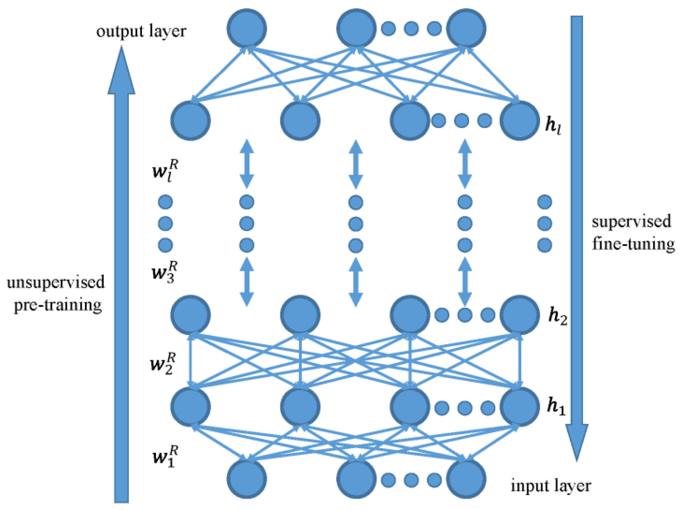
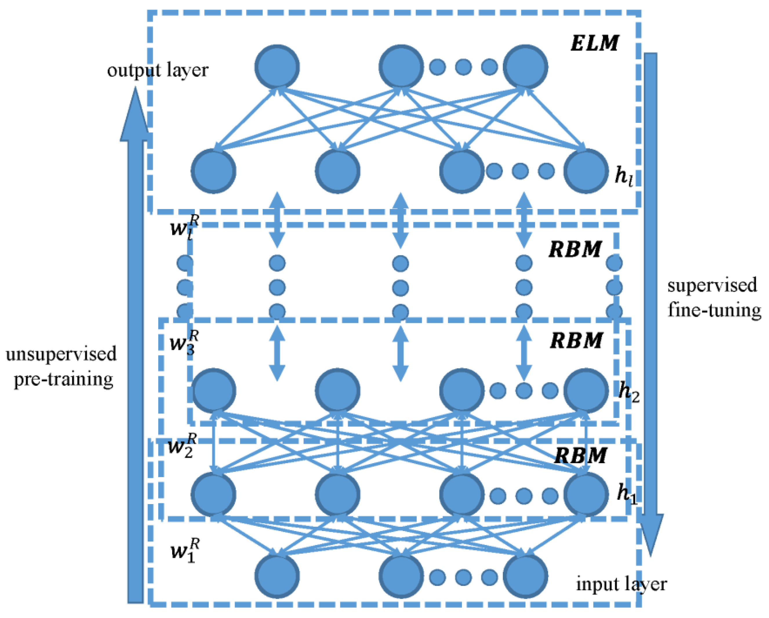
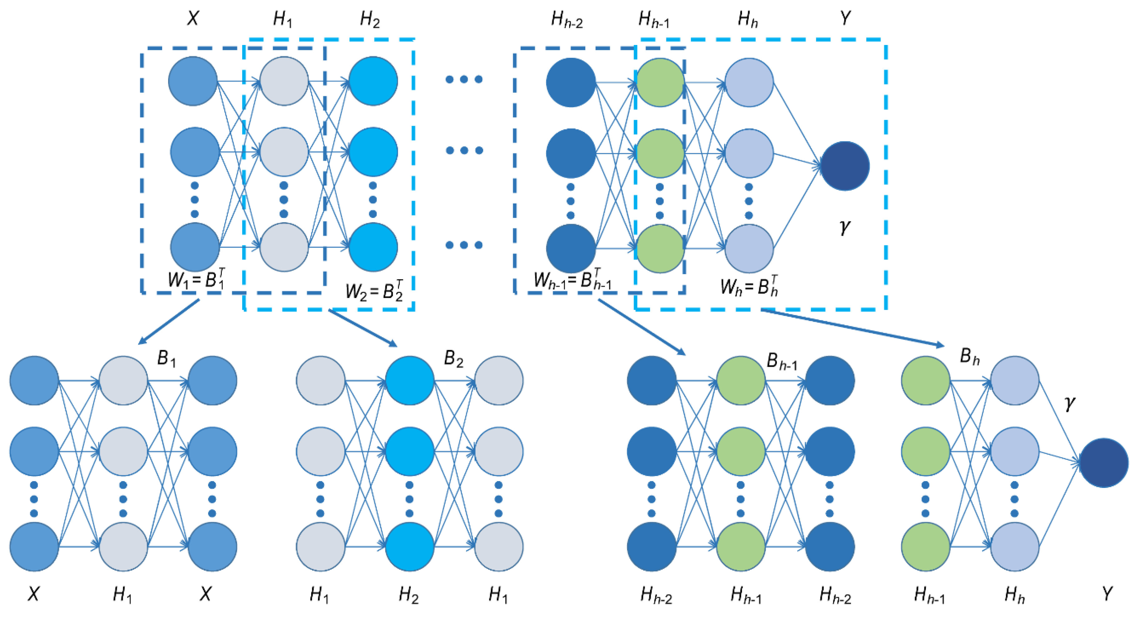
4.1. Soft Sensors for Extracting Deep Features

The deep belief network (DBN) achieves the approximation of complex functions through unsupervised layer-by-layer pre-training and supervised backpropagation fine-tuning [98,99]. In the process of unsupervised pre-training, the auxiliary variables are subjected to nonlinear mapping through the stacked restricted Boltzmann machine to extract the abstract features of the training samples. In the process of supervised backpropagation fine-tuning, the weights are fine-tuning through the backpropagation of the supervised signal to realize the further adjustment and optimization of the weights of the network.

To overcome the dependence of the traditional anaerobic digestion soft sensor on the features selection, Li proposed a soft sensor based on a deep belief network to predict the concentration of VFA for the anaerobic digestion process [100]. The structure diagram is illustrated in Figure 2.

The gradient descent algorithm cannot effectively train the deep network. Therefore, the contrast divergence (CD) algorithm is adopted to update the weights of the restricted Boltzmann machine, layer by layer:

$$\{\begin{array}{c}{w}_{ij}^R=w_{ij}^R+\eta \left(v_i^{\left(t-1\right)}{h}_j^{\left(t-1\right)}-v_i^{\left(t\right)}{h}_j^{\left(t\right)}\right)\\ b_j=b_j+\eta \left(h_j^{\left(t-1\right)}-h_j^{\left(t\right)}\right)\\ a_i=a_i+\eta \left(v_i^{\left(t-1\right)}-v_i^{\left(t\right)}\right)\end{array}$$

(20)

where v denotes the state vector of the visible layer, h refers to the state vector of the hidden layer, $\eta$ represents the learning rate, and w and b denote the weights and biases of the network, respectively. The soft sensor, with excellent feature learning capabilities, can effectively learn the essential features from the training samples and address the defects of excessive dependence on prior knowledge in feature selection.

However, the random setting of the weights of DBN’s output layer increases the randomness of the model’s prediction performance. To further improve the stability of prediction performance and generalization performance, Li proposed to adopt the extreme learning machine (ELM) algorithm after the weights of the first n-1 layers were obtained using the CD algorithm to determine the weights of the output layer, and establish a soft sensor based on an improved deep belief network (IDBN) to predict the VFA concentration. IDBN structure diagram is presented in Figure 3.

$$\beta =h_{n-1}{\left(w_i,{\widehat{b}}_i\right)}^{+}y$$

(21)

where $h_{n-1}{\left(w_i,{\widehat{b}}_i\right)}^{+}$ indicates the output of the hidden layer of the n-1 layer, β represents the weights of the output layer, and y denotes the VFA concentration. Compared with the soft sensor based on DBN, the improved soft sensor has preferable prediction accuracy and generalization performance in the experimental. However, the unsupervised layer-by-layer training process based on the CD algorithm requires a lot of iterative calculations, and the training process does not consider the mapping relationship between auxiliary variables and target variables. Therefore, Wang proposed a soft sensor based on the stacked supervised autoencoder combined with the kernel extreme learning machine (SSAE-KELM) algorithm to predict the VFA concentration [101]. The structure of SSAE-KELM is shown in Figure 4.

For the soft sensor, the ELM algorithm is employed to train supervised autoencoders (SAE), and the deep features of auxiliary variables are extracted through stacked SAE. The loss function of the training process is expressed as:

$$Loss=\frac{C_1}{2}\Vert X-H{r}_1\Vert {}_2^2+\frac{C_2}{2}\Vert Y-H{r}_2\Vert {}_2^2+\frac{1}{2}\Vert {r\Vert }_2^2$$

(22)

By minimizing the loss function, the output weight is obtained:

$$r={[C{H}^{T}H-I_{m+1}{}^{-1}{H}^{T}Y]}^T$$

(23)

where $X$ refers to the auxiliary variables; $Y$ represents the VFA concentration; $H$ denotes the hidden layer output; $r_1$ and $r_2$ indicate the hidden layer weights and the supervised item weights, respectively; $C_1$ and $C_2$ are the weight coefficients. Finally, the kernel extreme learning machine is adopted to establish a regression model to predict the VFA concentration on the extracted deep abstract features. Compared with soft sensors based on IDBN, the soft sensor introduces supervised items by improving the loss function. As a result, the soft sensor can extract the deep features of the auxiliary variable while considering the mapping relationship between the auxiliary variable and the VFA concentration. Then, it can extract the essential features that have a greater impact on the VFA concentration. Moreover, the ELM algorithm is used to compensate for the shortcomings of the slow training speed of the traditional CD algorithm and improve the training efficiency of the model.

4.2. Soft Sensors for Extracting Information from Unlabeled Samples

In the anaerobic digestion process, the long period and high cost of target variable collection make it difficult for soft sensors to obtain sufficient labeled samples [102]. However, there are many unlabeled samples composed of process variables in the industrial process. With the semi-supervised learning mechanism, the information of unlabeled samples can be fully mined, and the prediction accuracy and generalization ability of soft sensors are improved. In recent years, semi-supervised learning mechanisms have been widely used in deep neural networks. Therefore, Yan proposed a soft sensor based on the semi-supervised hierarchical extreme learning machine to predict VFA concentration in the anaerobic digestion process [103]. The model structure of the semi-supervised hierarchical extreme learning machine is illustrated in Figure 5.

Hierarchical extreme learning machine (HELM) is a multi-layer feedforward neural network composed of a multi-layer extreme learning machine-autoencoder (ELM-AE). During the training process, ELM-AE can achieve the lossless reconstruction of auxiliary variables. Therefore, the combined feature information of auxiliary variables can be extracted to a certain extent when the number of neurons in the hidden layer of ELM-AE is less than the number of neurons in the input layer [104]. The reconstruction loss function of ELM-AE is expressed as:

$$Loss=min\frac{1}{2}\Vert {\gamma \Vert }^2+\frac{C}{2}\Vert Y-J{\gamma \Vert }^2$$

(24)

The reconstruction loss function is minimized to obtain the output weight.

$$\gamma ={\left(J^{T}J+\frac{1}{C}{I}_n\right)}^{-1}{J}^{T}X$$

(25)

where $\gamma$ indicates the weight of the output layer of ELM-AE; $C$ is the weight factor; $J$ denotes the output of the hidden layer; $X$ and $Y$ represent auxiliary variables and VFA concentration, respectively. Manifold regularization is used as a semi-supervised learning mechanism to learn the distribution of unlabeled samples. It can preserve the manifold domain relationship between the data vectors in the original space. The essential idea of manifold regularization is to keep the local geometric structure of the original feature space in the new projection space. The loss function of HELM that introduces the manifold regularization term is:

$$Loss=min\frac{1}{2}\Vert {\gamma \Vert }^2+\frac{C}{2}\Vert Y-J{\gamma \Vert }^2+\frac{\lambda }{2}Tr\left({\widehat{Y}}^{T}L\widehat{Y}\right)$$

(26)

The loss function is minimized to acquire the output weight.

$$r={\left(I_n+C{J}^{T}J+\lambda H^{T}LH\right)}^{-1}C{J}^T$$

(27)

where $\gamma$ indicates the output layer weight of HELM; $\lambda$ is the weight factor; $Tr(·)$ represents the trace of the matrix; $L$ refers to the graph Laplacian matrix; $H$ and $\widehat{Y}$ denote the hidden layer output and prediction output of all samples, respectively. Compared with traditional soft sensors, soft sensors based on a semi-supervised learning mechanism can learn both unlabeled sample information and label sample information. The semi-supervised learning mechanism can make full use of many unlabeled samples in the industrial process, contributing to the improvement of the prediction accuracy and generalization ability of soft sensors.

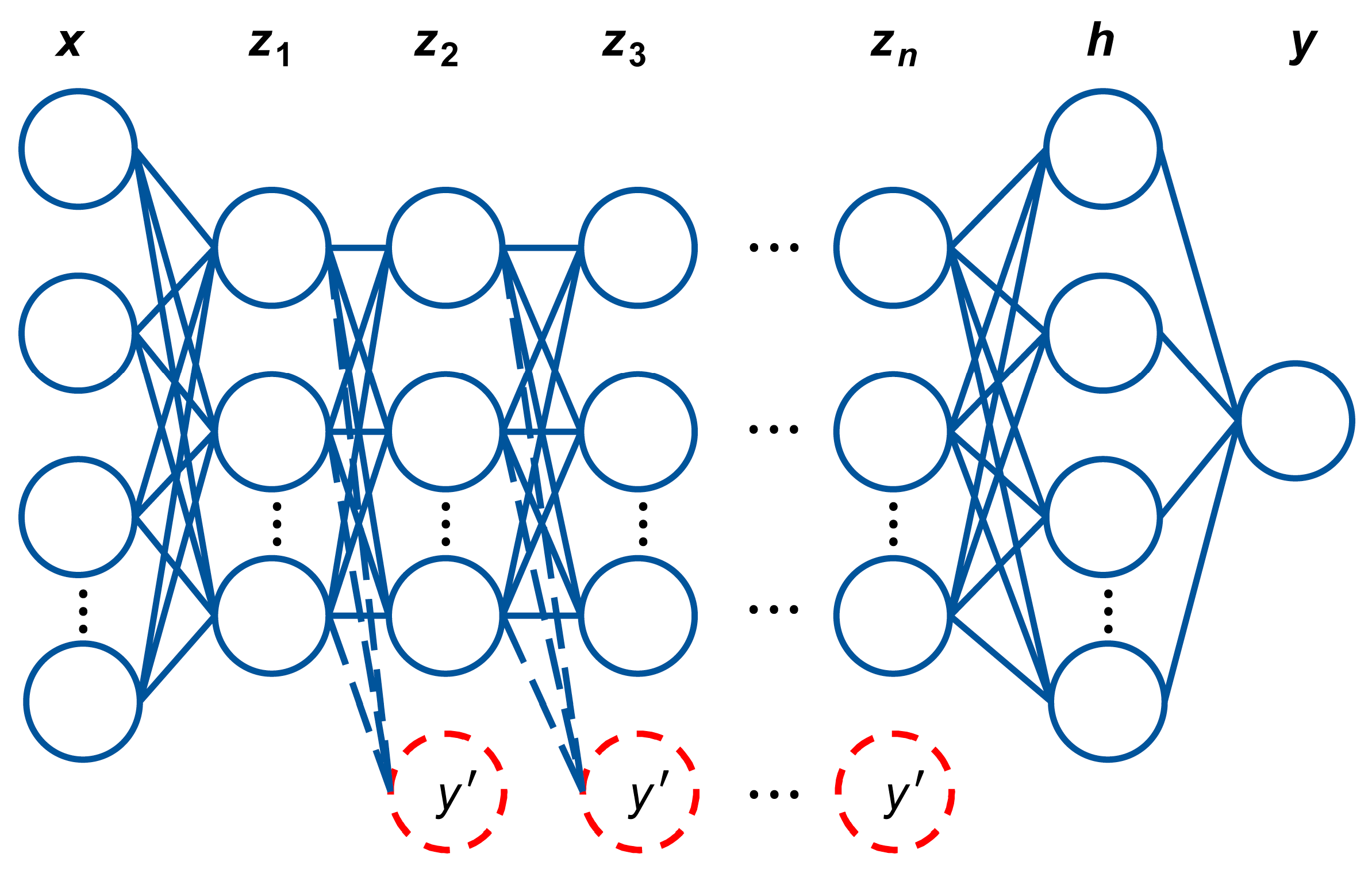
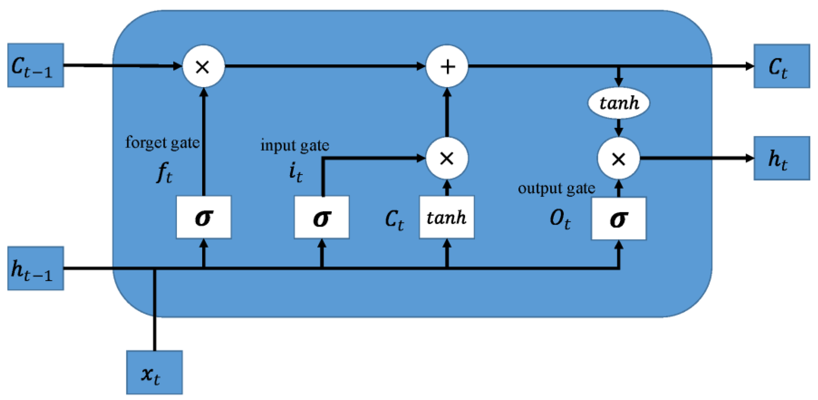
4.3. Soft Sensors for Extracting Dynamic Information

In the industrial production process of anaerobic digestion, changes in operating tasks, production materials, and production environment would cause changes in system operating conditions, making the prediction accuracy of soft sensors gradually decrease over time. Moreover, the different start-up times of the methane tank could lead to large differences in the digestion degree, substrate concentration, and biological activity, leading to inconsistent data distribution in the original data set. To handle this complication, Wang proposed to use the domain space transfer extreme learning machine (DSTELM) algorithm to adjust the data distribution [103]. The reconstruction loss function of DSTELM is:

$$loss=\frac{1}{2}\Vert {r\Vert }^2+\frac{c}{2}\Vert X_T-H_T{r\Vert }^2+\frac{\lambda }{2}Tr\left[r^T{H}^{T}MHr\right]$$

(28)

where $c$ and $\lambda$ are weighting factors; $r$ denotes the output weight; $X_T$ represents the auxiliary variables of the test set; $H=\left[H_S;H_T\right]$ indicates the output of the hidden layer; $Tr(·)$ refers to the trace of the matrix. The M is defined as:

$$M=\{\begin{array}{c}\frac{1}{n_S^2} i,j\le n_S\\ \frac{1}{n_T^2} i,j>n_S\\ \frac{1}{n_S{n}_T} other\end{array}$$

(29)

The loss function is minimized to obtain the output weight.

$$r={\left(I_L+H^T\left(C+\lambda M\right)H\right)}^{-1}{H}^{T}C{X}_T$$

(30)

where $C=diag\left(0_{n_S\times n_S},c,c,\dots ,c\right)$. The algorithm can minimize the distribution distance between the training set and the test set while retaining the essential characteristics of the test set. Moreover, it can address the problem of low model prediction accuracy caused by the inconsistent data distribution of the training set and the test set. Furthermore, a soft sensor based on the domain space migration hierarchical extreme learning machine (DSTHELM) is established by stacking DSTELM to extract the deep features of auxiliary variables. Compared with traditional soft sensors, soft sensors based on DSTHELM can better adapt to modal changes and data drift and thus present higher prediction accuracy and generalization ability.

Additionally, the hydrolysis reaction process is slow in the anaerobic digestion process, resulting in a certain time lag between the real-time monitoring variables of the acid-generating tank and the real-time monitoring variables of the methane generating tank. This suggests that the target variable is affected by the auxiliary variable in the current state, the changes in the operating conditions, and production conditions at the last moment, as well as the target variable in the current state. Therefore, Mccormick proposed a dynamic soft sensor based on long short-term memory (LSTM) network to predict biogas yield [105]. The LSTM structure is exhibited in Figure 6.

In the training process, the soft sensor realizes the retention or deletion of current information and historical information through the gate control unit. The input gate determines the extent to which the current input is retained to the current state. The forget gate determines the extent to which the state at the previous moment is retained to the current state. The output gate determines the extent to which the current state is retained to the output. The specific formulas are

$$i_t=\sigma \left(w_i·\left[h_{t-1},x_t\right]+b_i\right)$$

(31)

$$f_t=\sigma \left(w_f·\left[h_{t-1},x_t\right]+b_f\right)$$

(32)

$$h_t=\sigma \left(w_0·\left[h_{t-1},x_t\right]+b_0\right)$$

(33)

where $i_t$, $f_t$, $h_t$, and σ represent the input gate, the forget gate, the output gate, and the sigmoid activation function, respectively. The soft sensor can extract the different characteristics of the auxiliary variable at different times. Meanwhile, the soft sensor can retain historical biogas yield and its main influencing factors as auxiliary variables for current biogas yield forecasting, realizing the persistence of historical information.

The dynamic soft sensor considers the influence of historical data on the current state and overcomes the defect that the traditional soft sensor neglects the time scale information. Therefore, the dynamic soft sensor, to a certain extent, addresses the time lag caused by the slow reaction of the anaerobic digestion process. Furthermore, a dynamic soft sensor based on a combined convolutional neural network and long short-term memory network is established using the deep feature extraction ability of the convolutional neural network and the dynamic information extraction ability of LSTM to predict biogas yield. It can effectively extract the deep features of the data while using LSTM for timing error compensation. Thus, dynamic correction of the model is realized, and the prediction accuracy and generalization ability of the model are further improved.

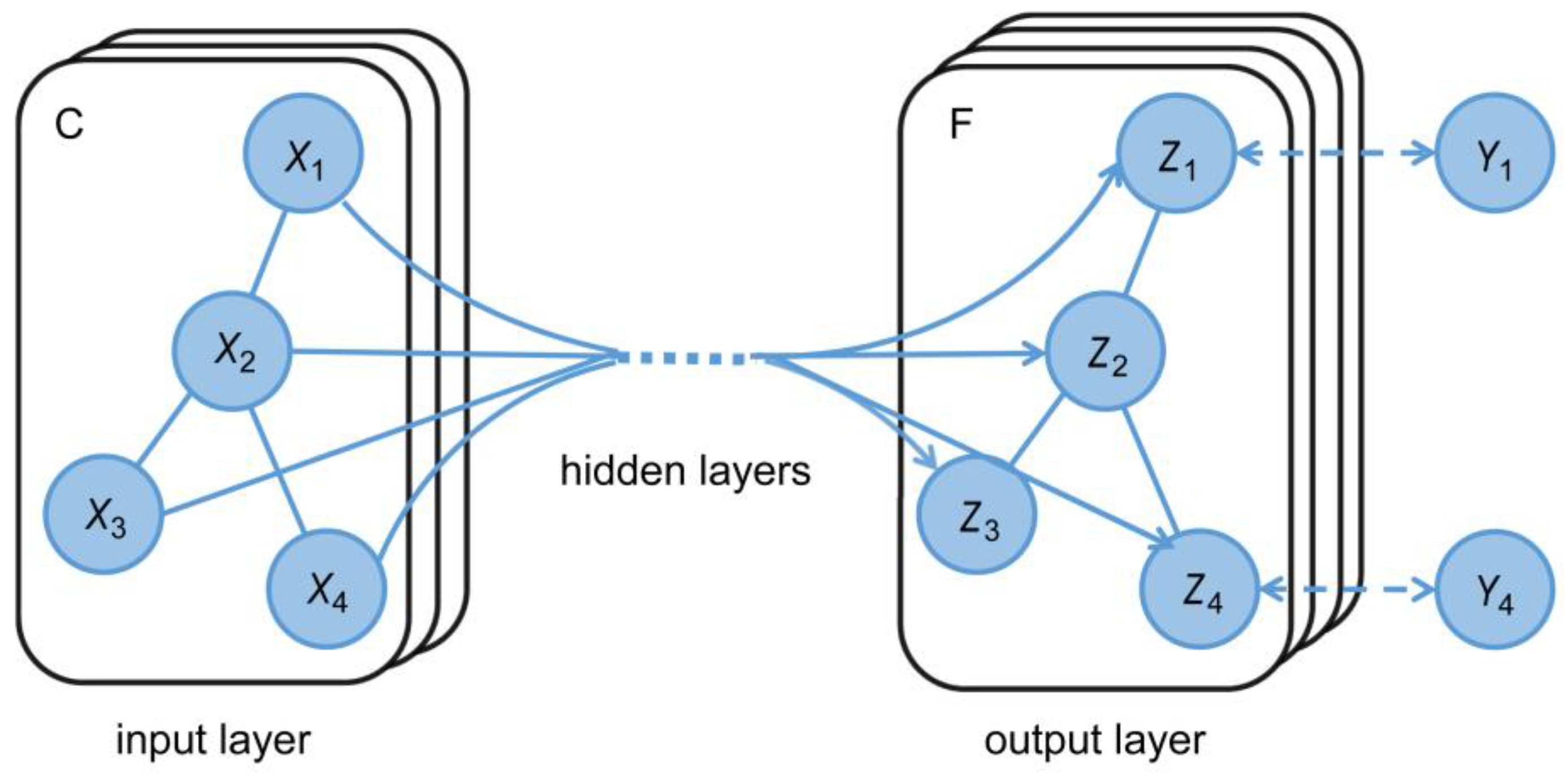
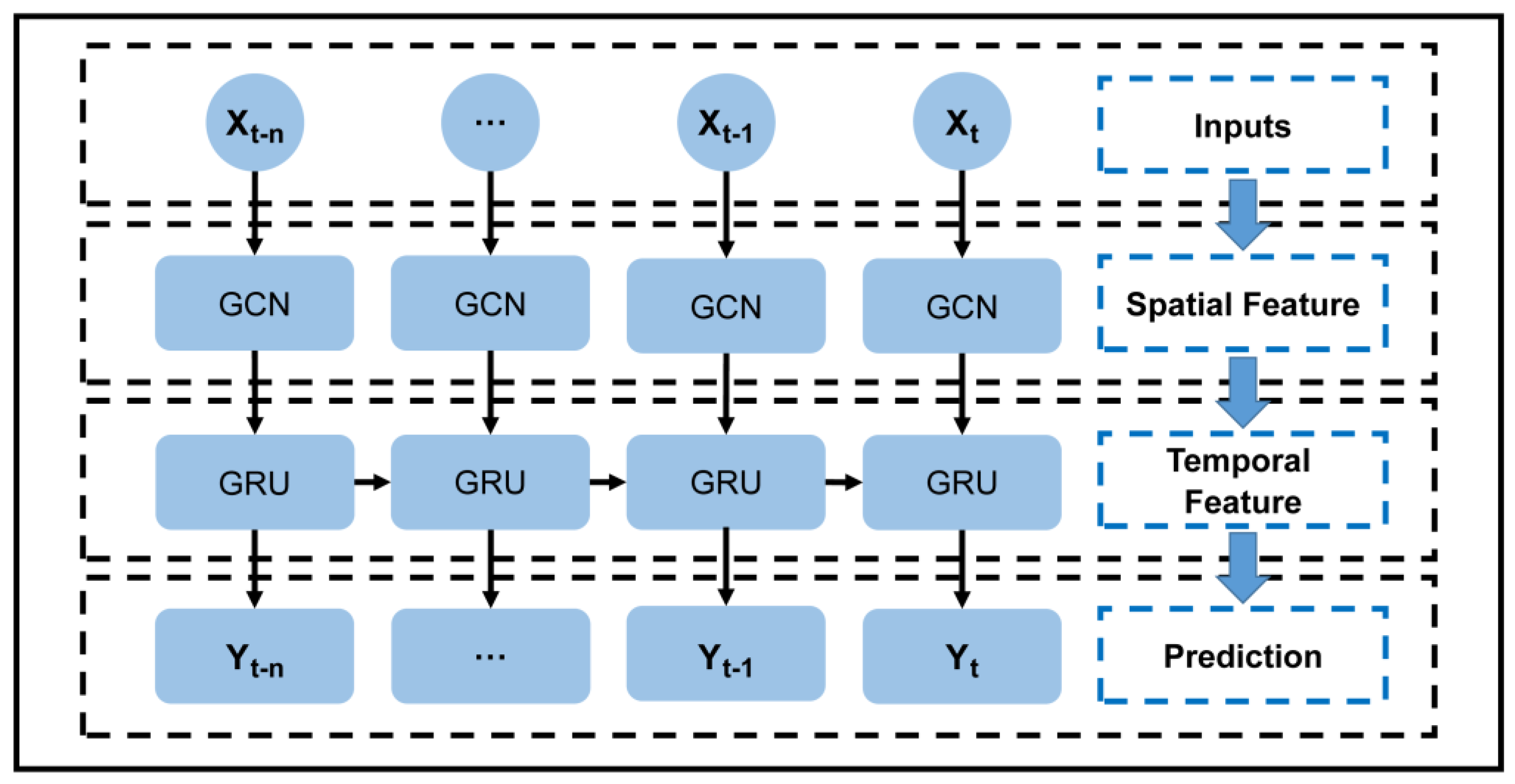
4.4. Soft Sensors for Extracting Spatiotemporal Information

In recent years, the graph convolutional network (GCN) has been widely used, owing to its powerful feature representation ability [106]. GCN can reduce the complexity of the soft sensor through the parameter sharing of the convolution kernel in the local area. Moreover, the adjacency matrix of the GCN enables the soft sensor to quantify the mutual influence between auxiliary variables, that is, considering the degree of influence of surrounding nodes on the target node and extracting the spatial information of the sample data. In the actual industry, the combined auxiliary variables are generally highly correlated with the target variable while the single auxiliary variable often has a weak correlation with the target variable. Therefore, researchers proposed a soft sensor based on GCN to predict VFA concentration [107]. The GCN structure is exhibited in Figure 7.

The output of the soft sensor can be expressed as:

$$Y=f\left(\widehat{A}XW\right)$$

(34)

where $X$ indicates the auxiliary variable; $Y$ refers to the output of the soft sensor; $f$ represents the nonlinear activation function; $\widehat{A}$ is the normalized adjacency matrix; $W$ denotes the learnable convolution kernel parameter. A proper adjacency matrix can be adopted to effectively extract the spatial information between auxiliary variables and improve the prediction accuracy and generalization ability of the soft sensor. Since the maximal information coefficient (MIC) can calculate the correlation between auxiliary variables, the normalized MIC is used to construct the adjacency matrix.

$$m_{ij}=MIC\left(x_i,x_j\right)$$

(35)

$${\alpha }_{ij}=\frac{exp(m_{ij})}{{{\displaystyle \sum }}_{k\in N_i}exp(m_{ik})}$$

(36)

where $m_{ij}$ represents the MIC between auxiliary variables $i$ and $j$; ${\alpha }_{ij}$ denotes the normalized MIC between auxiliary variables $i$ and $j$; $softmax$ indicates the normalization function. Compared with the traditional soft sensor, the soft sensor can learn the spatial information of the auxiliary variable by fully considering the influence of the combined feature information on the VFA concentration.

Given the dynamic characteristics and time lag characteristics of the anaerobic digestion process, a dynamic soft sensor based on the spatiotemporal graph convolutional network (STGCN) is established by introducing a gated recurrent unit (GRU). GRU can learn the dynamic changes of sample data to capture time information and consider the impact of historical sample information on current sample information. Therefore, this soft sensor can simultaneously consider the time information and spatial information of the anaerobic digestion process data. The structure of STGCN is presented in Figure 8.

During the training process, the STGCN can better handle the spatial and temporal characteristics of samples. The combined feature information of the sample is extracted using GCN to obtain its spatial dependence. Moreover, GRU is used to capture the dynamic change information of historical information and obtain temporal dependence. The specific calculation formulas are:

$$r_t=\sigma \left(W_r\left[h_{t-1},f(X_t,A)\right]\right)$$

(37)

$$z_t=\sigma \left(W_z\left[h_{t-1},f\left(X_t,A\right)\right]\right)$$

(38)

$${\tilde{h}}_t=tanh\left(W_{\tilde{h}}\left[r_t\odot h_{t-1},f(X_t,A)\right]\right)$$

(39)

$$h_t=\left(1-z_t\right)\odot h_{t-1}+z_t\odot {\tilde{h}}_t$$

(40)

where $A$ is the adjacency matrix; $f(X_t,A)$ represents the graph convolution process; $r_t$ denotes the reset gate; $z_t$ represents the update gate; $h$ refers to the state of the hidden layer; $\sigma$ is the activation function; $\odot$ represents the Hadamard product. Compared with the traditional soft sensor, the dynamic soft sensor based on STGCN can effectively extract the time information and spatial information from the anaerobic digestion process data, contributing to the achievement of the accurate prediction of the current VFA concentration.

5. Conclusions

The anaerobic digestion process is a time-varying, non-linear, and highly complex system with constraints. It is difficult to establish an accurate mechanism model to describe the anaerobic digestion process. The soft sensor based on regression analysis is more suitable for handling linear problems. However, there are strong nonlinear characteristics in the anaerobic digestion process. Soft sensors based on artificial neural networks are significantly affected by the network topology and the quality of training samples. They are prone to a local optimal or over-fitting state. Moreover, their generalization ability is weak. The soft sensor based on statistical learning is not suitable for processing large-scale data and is unable to monitor the anaerobic digestion process in real-time with high precision. However, soft sensors based on deep learning can learn essential features from training samples, introduce a semi-supervised learning mechanism to fully use unlabeled sample information, consider the dynamic characteristics in actual working conditions and the mutual mapping relationship between auxiliary variables, and extract the time information and space information of the sample data. Therefore, the soft sensor based on deep learning has higher prediction accuracy and generalization ability. The general idea of this paper is illustrated in Figure 9.

At present, a soft sensor for anaerobic digestion based on deep learning can be further developed. In the industrial production process, the mechanism model is combined with deep learning to enhance the interpretability of the soft sensor and realize the closed-loop guidance of the industrial process. Furthermore, the difficulty of sample collection during anaerobic digestion hinders researchers to obtain enough samples to train soft sensors. Therefore, constructing generated samples by the generative adversarial network is an effective solution for the shortage of soft sensor training samples.

References

1. Yang, H.; Mo, W.-l.; Xiong, Z.-X.; Huang, M.-Z.; Liu, H.-B. Soft sensor modeling of papermaking effluent treatment processes using RPLS. China Pulp Pap. 2018, 35, 31–35. [Google Scholar] [CrossRef]
2. Yordanova, S.; Noikova, N.; Petrova, R.; Tzvetkov, P. Neuro-fuzzy modelling on experimental data in anaerobic digestion of organic waste in waters. In Proceedings of the 2005 IEEE Intelligent Data Acquisition and Advanced Computing Systems: Technology and Applications, Sofia, Bulgaria, 5–7 September 2005; pp. 84–88. [Google Scholar]
3. Liu, Z.-J.; Wan, J.-Q.; Ma, Y.-W.; Wang, Y. Online prediction of effluent COD in the anaerobic wastewater treatment system based on PCA-LSSVM algorithm. Env. Sci. Pollut. Res. Int. 2019, 26, 12828–12841. [Google Scholar] [CrossRef] [PubMed]
4. Bryant, M.P.; Wolin, E.A.; Wolin, M.J.; Wolfe, R.S. Methanobacillus omelianskii, a symbiotic association of two species of bacteria. Arch. Mikrobiol. 1967, 59, 20–31. [Google Scholar] [CrossRef] [PubMed]
5. Bryant, M.P. Microbial methane production—theoretical aspects. J. Anim. Sci. 1979, 48, 193–201. [Google Scholar] [CrossRef]
6. Franke-Whittle, I.H.; Walter, A.; Ebner, C.; Insam, H. Investigation into the effect of high concentrations of volatile fatty acids in anaerobic digestion on methanogenic communities. Waste Manag. 2014, 34, 2080–2089. [Google Scholar] [CrossRef] [Green Version]
7. Sbarciog, M.; Loccufier, M.; Noldus, E. Determination of appropriate operating strategies for anaerobic digestion systems. Biochem. Eng. J. 2010, 51, 180–188. [Google Scholar] [CrossRef]
8. Shen, S.; Premier, G.C.; Guwy, A.; Dinsdale, R. Bifurcation and stability analysis of an anaerobic digestion model. Nonlinear Dyn. 2007, 48, 391–408. [Google Scholar] [CrossRef]
9. Lara-Cisneros, G.; Aguilar-López, R.; Femat, R. On the dynamic optimization of methane production in anaerobic digestion via extremum-seeking control approach. Comput. Chem. Eng. 2015, 75, 49–59. [Google Scholar] [CrossRef]
10. Corona, F.; Mulas, M.; Haimi, H.; Sundell, L.; Heinonen, M.; Vahala, R. Monitoring nitrate concentrations in the denitrifying post-filtration unit of a municipal wastewater treatment plant. J. Process Control 2013, 23, 158–170. [Google Scholar] [CrossRef]
11. Jimenez, J.; Latrille, E.; Harmand, J.; Robles, A.; Ferrer, J.; Gaida, D.; Wolf, C.; Mairet, F.; Bernard, O.; Alcaraz-Gonzalez, V.; et al. Instrumentation and control of anaerobic digestion processes: A review and some research challenges. Rev. Environ. Sci. Biotechnol. 2015, 14, 615–648. [Google Scholar] [CrossRef]
12. Kawai, M.; Nagao, N.; Kawasaki, N.; Imai, A.; Toda, T. Improvement of COD removal by controlling the substrate degradability during the anaerobic digestion of recalcitrant wastewater. J. Environ. Manag. 2016, 181, 838–846. [Google Scholar] [CrossRef]
13. Gaida, D.; Wolf, C.; Meyer, C.; Stuhlsatz, A.; Lippel, J.; Bäck, T.; Bongards, M.; McLoone, S. State estimation for anaerobic digesters using the ADM1. Water Sci. Technol. 2012, 66, 1088–1095. [Google Scholar] [CrossRef] [PubMed]
14. Haimi, H.; Mulas, M.; Corona, F.; Vahala, R. Data-derived soft-sensors for biological wastewater treatment plants: An overview. Environ. Model. Softw. 2013, 47, 88–107. [Google Scholar] [CrossRef]
15. Gaida, D.; Wolf, C.; Bongards, M. Feed control of anaerobic digestion processes for renewable energy production: A review. Renew. Sustain. Energy Rev. 2017, 68, 869–875. [Google Scholar] [CrossRef]
16. Langergraber, G.; Fleischmann, N.; Hofstaedter, F.; Weingartner, A. Monitoring of a paper mill wastewater treatment plant using UV/VIS spectroscopy. Water Sci. Technol. 2004, 49, 9–14. [Google Scholar] [CrossRef] [PubMed]
17. Han, D.; Zou, Z. Soft sensor and inferential control technology. J. Nanjing Univ. Sci. Technol. 2005, 212–216. [Google Scholar] [CrossRef]
18. Wade, M.J. Not just numbers: Mathematical modelling and its contribution to anaerobic digestion processes. Processes 2020, 8, 888. [Google Scholar] [CrossRef]
19. Brosilow, C.; Tong, M. Inferential control of processes: Part II. The structure and dynamics of inferential control systems. AIChE 1978, 24, 492–500. [Google Scholar] [CrossRef]
20. He, B.; Zhu, X. Soft-sensing technique based on extension method. In Proceedings of the SPIE 5253, Fifth International Symposium on Instrumentation and Control Technology, Beijing, China, 24–27 October 2003; pp. 38–42. [Google Scholar]
21. Wang, Z.-x.; Liu, Z.-w.; Xue, F.-x. Soft sensing technique for sewage treatment process. J. Beijing Technol. Bus. Univ. 2005, 23, 31–34. [Google Scholar] [CrossRef]
22. Yu, J.; Zhou, C. Soft-sensing techniques in process control. Control Theory Appl. 1996, 137–144. [Google Scholar]
23. Zhu, X. Soft-sensing technique and its applications. J. South China Univ. Technol. 2002, 30, 61–67. [Google Scholar] [CrossRef]
24. James, S.C.; Legge, R.L.; Budman, H. On-line estimation in bioreactors: A review. Rev. Chem. Eng. 2000, 16, 311–340. [Google Scholar] [CrossRef]
25. Kadlec, P.; Gabrys, B.; Strandt, S. Data-driven soft sensors in the process industry. Comput. Chem. Eng. 2009, 33, 795–814. [Google Scholar] [CrossRef] [Green Version]
26. Zeikus, J. Microbial populations in digesters. In Proceedings of the First International Symposium on Anaerobic Digestion, London, UK, 17–21 September 1979. [Google Scholar]
27. Keymer, P.; Ruffell, I.; Pratt, S.; Lant, P. High pressure thermal hydrolysis as pre-treatment to increase the methane yield during anaerobic digestion of microalgae. Bioresour. Technol. 2013, 131, 128–133. [Google Scholar] [CrossRef]
28. Appels, L.; Baeyens, J.; Degrève, J.; Dewil, R. Principles and potential of the anaerobic digestion of waste-activated sludge. Prog. Energy Combust. Sci. 2008, 34, 755–781. [Google Scholar] [CrossRef]
29. Illi, L.; Lecker, B.; Lemmer, A.; Müller, J.; Oechsner, H. Biological methanation of injected hydrogen in a two-stage anaerobic digestion process. Bioresour. Technol. 2021, 333, 125126. [Google Scholar] [CrossRef]
30. Kazemi, P.; Bengoa, C.; Steyer, J.-P.; Giralt, J. Data-driven techniques for fault detection in anaerobic digestion process. Process Saf. Environ. Prot. 2021, 146, 905–915. [Google Scholar] [CrossRef]
31. Boe, K. Online Monitoring and Control of the Biogas Process; Institute of Environment & Resources, Technical University of Denmark: Copenhagen, Denmark, 2006. [Google Scholar]
32. Hwang, M.H.; Jang, N.J.; Hyun, S.H.; Kim, I.S. Anaerobic bio-hydrogen production from ethanol fermentation: The role of pH. J. Biotechnol. 2004, 111, 297–309. [Google Scholar] [CrossRef] [PubMed]
33. Stichting Toegepast Onderzoek Reiniging Afvalwater. Optimalisatie van de Gistingsgasproduktie; Stora: Amsterdam, The Netherlands, 1985. [Google Scholar]
34. Turovskiy, I.S.; Mathai, P. Wastewater Sludge Processing; John Wiley & Sons: Hoboken, NJ, USA, 2006. [Google Scholar]
35. Steyer, J.P.; Bouvier, J.C.; Conte, T.; Gras, P.; Harmand, J.; Delgenes, J.P. On-line measurements of COD, TOC, VFA, total and partial alkalinity in anaerobic digestion processes using infra-red spectrometry. Water Sci. Technol. 2002, 45, 133–138. [Google Scholar] [CrossRef] [PubMed]
36. Chae, K.J.; Jang, A.; Yim, S.K.; Kim, I.S. The effects of digestion temperature and temperature shock on the biogas yields from the mesophilic anaerobic digestion of swine manure. Bioresour. Technol. 2008, 99, 1–6. [Google Scholar] [CrossRef]
37. Massi, E. Anaerobic digestion. In Fuel Cells in the Waste-to-Energy Chain: Distributed Generation through Non-Conventional Fuels and Fuel Cells; McPhail, S.J., Cigolotti, V., Moreno, A., Eds.; Springer: London, UK, 2012; pp. 47–63. [Google Scholar]
38. Ren, Y.; Yu, M.; Wu, C.; Wang, Q.; Gao, M.; Huang, Q.; Liu, Y. A comprehensive review on food waste anaerobic digestion: Research updates and tendencies. Bioresour. Technol. 2018, 247, 1069–1076. [Google Scholar] [CrossRef]
39. Liu, X.; Han, Z.; Yang, J.; Ye, T.; Yang, F.; Wu, N.; Bao, Z. Review of enhanced processes for anaerobic digestion treatment of sewage sludge. IOP Conf. Ser. Earth Environ. Sci. 2018, 113, 012039. [Google Scholar] [CrossRef]
40. Ye, N.-F.; He, P.-J.; Lü, F.; Shao, L.-M. Effect of pH on microbial diversity and product distribution during anaerobic fermentation of vegetable waste. Chin. J. Appl. Environ. Biol. 2007, 13, 238–242. [Google Scholar] [CrossRef]
41. Adekunle, K.F.; Okolie, J.A. A review of biochemical process of anaerobic digestion. Adv. Biosci. Biotechnol. 2015, 6, 205–212. [Google Scholar] [CrossRef] [Green Version]
42. Khalid, A.; Arshad, M.; Anjum, M.; Mahmood, T.; Dawson, L. The anaerobic digestion of solid organic waste. Waste Manag. 2011, 31, 1737–1744. [Google Scholar] [CrossRef] [PubMed]
43. Lettinga, G. Anaerobic digestion and wastewater treatment systems. Antonie Van Leeuwenhoek 1995, 67, 3–28. [Google Scholar] [CrossRef] [PubMed]
44. Mumme, J.; Linke, B.; Tölle, R. Novel upflow anaerobic solid-state (UASS) reactor. Bioresour. Technol. 2010, 101, 592–599. [Google Scholar] [CrossRef]
45. Angelidaki, I.; Chen, X.; Cui, J.; Kaparaju, P.; Ellegaard, L. Thermophilic anaerobic digestion of source-sorted organic fraction of household municipal solid waste: Start-up procedure for continuously stirred tank reactor. Water Res. 2006, 40, 2621–2628. [Google Scholar] [CrossRef]
46. Tufaner, F.; Avşar, Y. Investigation of biogas production potential and adaptation to cattle manure of anaerobic flocular sludge seed. Sigma 2016, 7, 183–190. [Google Scholar]
47. Dalkılıc, K.; Ugurlu, A. Biogas production from chicken manure at different organic loading rates in a mesophilic-thermopilic two stage anaerobic system. J. Biosci. Bioeng. 2015, 120, 315–322. [Google Scholar] [CrossRef] [PubMed]
48. Moral, H.; Aksoy, A.; Gokcay, C.F. Modeling of the activated sludge process by using artificial neural networks with automated architecture screening. Comput. Chem. Eng. 2008, 32, 2471–2478. [Google Scholar] [CrossRef]
49. Güçlü, D.; Dursun, S. Amelioration of carbon removal prediction for an activated sludge process using an artificial neural network (ANN). CLEAN–Soil Air Water 2008, 36, 781–787. [Google Scholar] [CrossRef]
50. Fang, F.; Ni, B.-J.; Yu, H.-Q. Estimating the kinetic parameters of activated sludge storage using weighted non-linear least-squares and accelerating genetic algorithm. Water Res. 2009, 43, 2595–2604. [Google Scholar] [CrossRef] [PubMed]
51. Batstone, D.J.; Keller, J.; Angelidaki, I.; Kalyuzhnyi, S.V.; Pavlostathis, S.G.; Rozzi, A.; Sanders, W.T.M.; Siegrist, H.; Vavilin, V.A. The IWA anaerobic digestion model No 1 (ADM1). Water Sci. Technol. 2002, 45, 65–73. [Google Scholar] [CrossRef]
52. Bernard, O.; Hadj-Sadok, Z.; Dochain, D. Software sensors to monitor the dynamics of microbial communities: Application to anaerobic digestion. Acta Biotheor. 2000, 48, 197–205. [Google Scholar] [CrossRef]
53. Fan, Q.; Qin, G.; Zhang, L. Research and application on hybrid modeling for the monitoring of anaerobic-thermophilic fermentation of cattle manure. Heilongjiang Sci. 2013, 45–47. [Google Scholar] [CrossRef]
54. Luenberger, D. An introduction to observers. IEEE Trans. Automat. Contr. 1971, 16, 596–602. [Google Scholar] [CrossRef]
55. Mohd Ali, J.; Ha Hoang, N.; Hussain, M.A.; Dochain, D. Review and classification of recent observers applied in chemical process systems. Comput. Chem. Eng. 2015, 76, 27–41. [Google Scholar] [CrossRef] [Green Version]
56. Bastin, G. On-Line Estimation and Adaptive Control of Bioreactors; Elsevier: Amsterdam, The Netherlands, 2013; Volume 1. [Google Scholar]
57. Dochain, D. State and parameter estimation in chemical and biochemical processes: A tutorial. J. Process Control 2003, 13, 801–818. [Google Scholar] [CrossRef]
58. Diop, S.; Simeonov, I. On the biomass specific growth rates estimation for anaerobic digestion using differential algebraic techniques. Bioautomation 2009, 13, 47–56. [Google Scholar]
59. Stanke, M.; Hitzmann, B. Automatic control of bioprocesses. In Measurement, Monitoring, Modelling and Control of Bioprocesses; Mandenius, C.-F., Titchener-Hooker, N.J., Eds.; Springer: Berlin/Heidelberg, Germany, 2013; pp. 35–63. [Google Scholar]
60. Kalchev, B.; Simeonov, I.; Christov, N. Kalman filter design for a second-order model of anaerobic digestion. Int. J. Bioautomation 2011, 15, 85–100. [Google Scholar]
61. Rodríguez, A.; Quiroz, G.; Femat, R.; Méndez-Acosta, H.O.; de León, J. An adaptive observer for operation monitoring of anaerobic digestion wastewater treatment. Chem. Eng. J. 2015, 269, 186–193. [Google Scholar] [CrossRef]
62. Lara-Cisneros, G.; Aguilar-López, R.; Dochain, D.; Femat, R. On-line estimation of VFA concentration in anaerobic digestion via methane outflow rate measurements. Comput. Chem. Eng. 2016, 94, 250–256. [Google Scholar] [CrossRef]
63. Haugen, F.; Bakke, R.; Lie, B. State estimation and model-based control of a pilot anaerobic digestion reactor. J. Control Sci. Eng. 2014, 2014, 572621. [Google Scholar] [CrossRef] [Green Version]
64. Benyahia, B.; Sari, T.; Cherki, B.; Harmand, J. Bifurcation and stability analysis of a two step model for monitoring anaerobic digestion processes. J. Process Control 2012, 22, 1008–1019. [Google Scholar] [CrossRef] [Green Version]
65. Hess, J.; Bernard, O. Design and study of a risk management criterion for an unstable anaerobic wastewater treatment process. J. Process Control 2008, 18, 71–79. [Google Scholar] [CrossRef]
66. Sbarciog, M.; Loccufier, M.; Vande Wouwer, A. On the optimization of biogas production in anaerobic digestion systems. IFAC Proc. Vol. 2011, 44, 7150–7155. [Google Scholar] [CrossRef] [Green Version]
67. Schaum, A.; Alvarez, J.; Garcia-Sandoval, J.P.; Gonzalez-Alvarez, V.M. On the dynamics and control of a class of continuous digesters. J. Process Control 2015, 34, 82–96. [Google Scholar] [CrossRef]
68. Eberly, L.E. Multiple linear regression. In Topics in Biostatistics; Ambrosius, W.T., Ed.; Humana Press: Totowa, NJ, USA, 2007; pp. 165–187. [Google Scholar]
69. Hu, K.-Q.; Li, L.-H.; Sun, Y.-M.; Kong, X.-Y.; Zhang, Y.; Yuan, Z.-H. The methane yield forecasting model of energy crops in anaerobic digestion based on feedstock components. Adv. New Renew. Energy 2016, 4, 100–104. [Google Scholar] [CrossRef]
70. Zhang, W.; Zhang, L.; Li, N.; Zhou, H. Comparing multiple regression and BP artificial nerve net model used on prediction of anaerobic co-digestion gas-producing process. Chin. J. Environ. Eng. 2013, 7, 747–752. [Google Scholar]
71. Mejdell, T.; Skogestad, S. Estimation of distillation compositions from multiple temperature measurements using partial-least-squares regression. Ind. Eng. Chem. Res. 1991, 30, 2543–2555. [Google Scholar] [CrossRef]
72. Tufaner, F.; Avşar, Y.; Gönüllü, M.T. Modeling of biogas production from cattle manure with co-digestion of different organic wastes using an artificial neural network. Clean Techn. Environ. Policy 2017, 19, 2255–2264. [Google Scholar] [CrossRef]
73. Güçlü, D.; Yılmaz, N.; Ozkan-Yucel, U.G. Application of neural network prediction model to full-scale anaerobic sludge digestion. J. Chem. Technol. Biotechnol. 2011, 86, 691–698. [Google Scholar] [CrossRef]
74. Holubar, P.; Zani, L.; Hager, M.; Fröschl, W.; Radak, Z.; Braun, R. Advanced controlling of anaerobic digestion by means of hierarchical neural networks. Water Res. 2002, 36, 2582–2588. [Google Scholar] [CrossRef]
75. Strik, D.P.B.T.B.; Domnanovich, A.M.; Zani, L.; Braun, R.; Holubar, P. Prediction of trace compounds in biogas from anaerobic digestion using the MATLAB Neural Network Toolbox. Environ. Model. Softw. 2005, 20, 803–810. [Google Scholar] [CrossRef]
76. Ozkaya, B.; Demir, A.; Bilgili, M.S. Neural network prediction model for the methane fraction in biogas from field-scale landfill bioreactors. Environ. Model. Softw. 2007, 22, 815–822. [Google Scholar] [CrossRef]
77. Sathish, S.; Vivekanandan, S. Parametric optimization for floating drum anaerobic bio-digester using response surface methodology and artificial neural network. Alex. Eng. J. 2016, 55, 3297–3307. [Google Scholar] [CrossRef] [Green Version]
78. Holubar, P.; Zani, L.; Hagar, M.; Fröschl, W.; Radak, Z.; Braun, R. Modelling of anaerobic digestion using self-organizing maps and artificial neural networks. Water Sci. Technol. 2000, 41, 149–156. [Google Scholar] [CrossRef]
79. Jacob, S.; Banerjee, R. Modeling and optimization of anaerobic codigestion of potato waste and aquatic weed by response surface methodology and artificial neural network coupled genetic algorithm. Bioresour. Technol. 2016, 214, 386–395. [Google Scholar] [CrossRef]
80. Abu Qdais, H.; Bani Hani, K.; Shatnawi, N. Modeling and optimization of biogas production from a waste digester using artificial neural network and genetic algorithm. Resour. Conserv. Recycl. 2010, 54, 359–363. [Google Scholar] [CrossRef]
81. Lu, J.-J.; Chen, H. Researching development on BP neural networks. Control Eng. China 2006, 13, 449–451. [Google Scholar] [CrossRef]
82. Yilmaz, T.; Seckin, G.; Yuceer, A. Modeling of effluent COD in UAF reactor treating cyanide containing wastewater using artificial neural network approaches. Adv. Eng. Softw. 2010, 41, 1005–1010. [Google Scholar] [CrossRef]
83. Han, W.; Huang, M.-z.; Ma, Y.-w.; Wan, J.-q. Multi-objective optimization in the anaerobic digestion of papermaking wastewater based on NSGA-2 and BP neural network. Pap. Sci. Technol. 2014, 33, 145–147, 165. [Google Scholar]
84. Huang, M.; Han, W.; Wan, J.; Ma, Y.; Chen, X. Multi-objective optimization for design and operation of anaerobic digestion using GA-ANN and NSGA-II. J. Chem. Technol. Biotechnol. 2016, 91, 226–233. [Google Scholar] [CrossRef]
85. Hua, Y.; Zhao, X.; Wang, X.; Teng, K. Prediction modeling for gas production of anaerobic fermentation based on improved BP neural network. Chin. J. Environ. Eng. 2016, 10, 5951–5956. [Google Scholar] [CrossRef]
86. Behera, S.K.; Meher, S.K.; Park, H.-S. Artificial neural network model for predicting methane percentage in biogas recovered from a landfill upon injection of liquid organic waste. Clean Techn. Environ. Policy 2015, 17, 443–453. [Google Scholar] [CrossRef]
87. Zhao, X.; Jiang, J. BP neural network modeling and particle swarm algorithm optimization of anaerobic fermentation process. Appl. Energy Technol. 2015, 8–12. [Google Scholar] [CrossRef]
88. Liu, L.; Xie, B.; Ma, Y.; Wan, J.; Wang, Y. Hybrid model of measuring biogas yield in anaerobic digestion process based on incorporated bio-kinetic model with support vector machine model. China Pulp Pap. 2017, 36, 31–36. [Google Scholar] [CrossRef]
89. Kazemi, P.; Steyer, J.-P.; Bengoa, C.; Font, J.; Giralt, J. Robust data-driven soft sensors for online monitoring of volatile fatty acids in anaerobic digestion processes. Processes 2020, 8, 67. [Google Scholar] [CrossRef] [Green Version]
90. Liu, L.; Ma, Y.; Wan, J.; Wang, Y.; Xie, B.; Wu, S. An accuracy soft-sensing model for the estimation of anaerobic digestion process based on pso-SVM model. Acta Sci. Circumstantiae 2017, 37, 2122–2129. [Google Scholar] [CrossRef]
91. Cui, G.; Sun, T.; Zhang, Y. Forecast of blast furnace hot metal temperature based on least support vector machine. Comput. Simul. 2013, 30, 354–357. [Google Scholar] [CrossRef]
92. Sun, J.; Cheng, Z.; Yang, R.; Shan, S. Soft-sensor modeling for paper mill effluent COD based on PCA-PSO-LSSVM. Comput. Appl. Chem. 2017, 34, 706–710. [Google Scholar] [CrossRef]
93. Xing, Y.; Cheng, Z.; Shan, S. Dynamic soft sensing of organic pollutants in effluent from UMIC anaerobic reactor for industrial papermaking wastewater. IOP Conf. Ser. Mater. Sci. Eng. 2019, 490, 062027. [Google Scholar] [CrossRef]
94. Du, X.; Cai, Y.; Wang, S.; Zhang, L. Overview of deep learning. In Proceedings of the 31st Youth Academic Annual Conference of Chinese Association of Automation (YAC), Wuhan, China, 11–13 November 2016; pp. 159–164. [Google Scholar]
95. Yao, L.; Ge, Z. Deep learning of semisupervised process data with hierarchical extreme learning machine and soft sensor application. ITIE 2018, 65, 1490–1498. [Google Scholar] [CrossRef]
96. Yuan, X.; Li, L.; Shardt, Y.A.W.; Wang, Y.; Yang, C. Deep learning with spatiotemporal attention-based LSTM for industrial soft sensor model development. ITIE 2021, 68, 4404–4414. [Google Scholar] [CrossRef]
97. Cao, Y.; Liu, C.; Huang, Z.; Sheng, Y.; Ju, Y. Skeleton-based action recognition with temporal action graph and temporal adaptive graph convolution structure. Multimed. Tools Appl. 2021. [Google Scholar] [CrossRef]
98. Bengio, Y. Learning Deep Architectures for AI; Now Publishers Inc.: Hanover, MA, USA, 2009. [Google Scholar]
99. Song, H.A.; Lee, S.-Y. Hierarchical representation using NMF. In Proceedings of the Neural Information Processing, Berlin, Heidelberg, 3 November 2013; pp. 466–473. [Google Scholar]
100. Wang, Y.; Li, X. Soft measurement for VFA concentration in anaerobic digestion for treating kitchen waste based on improved DBN. IEEE Access 2019, 7, 60931–60939. [Google Scholar] [CrossRef]
101. Wang, Y.; Wang, S. Soft sensor for VFA concentration in anaerobic digestion process for treating kitchen waste based on SSAE-KELM. IEEE Access 2021, 9, 36466–36474. [Google Scholar] [CrossRef]
102. Wang, X.; Liu, H. Data supplement for a soft sensor using a new generative model based on a variational autoencoder and Wasserstein GAN. J. Process Control 2020, 85, 91–99. [Google Scholar] [CrossRef]
103. Yan, P.; Shen, B.; Wang, Y. Soft sensor for VFA concentration in anaerobic digestion process for treating kitchen waste based on DSTHELM. IEEE Access 2020, 8, 223618–223625. [Google Scholar] [CrossRef]
104. Ranzato, M.; Huang, F.J.; Boureau, Y.; LeCun, Y. Unsupervised learning of invariant feature hierarchies with applications to object recognition. In Proceedings of the 2007 IEEE Conference on Computer Vision and Pattern Recognition, Minneapolis, MN, USA, 17–22 June 2007; pp. 1–8. [Google Scholar]
105. McCormick, M.; Villa, A.E.P. LSTM and 1-D convolutional neural networks for predictive monitoring of the anaerobic digestion process. In Proceedings of the Artificial Neural Networks and Machine Learning–ICANN 2019: Workshop and Special Sessions, Cham, Switzerland, 9 September 2019; pp. 725–736. [Google Scholar]
106. Zhuang, C.; Ma, Q. Dual graph convolutional networks for graph-based semi-supervised classification. In Proceedings of the Proceedings of the 2018 World Wide Web Conference, Lyon, France, 10 April 2018; pp. 499–508. [Google Scholar]
107. Wang, Y.; Yan, P.; Gai, M. Dynamic soft sensor for anaerobic digestion of kitchen waste based on SGSTGAT. IEEE Sens. J. 2021, 1. [Google Scholar] [CrossRef]
Figure 1. Two-phase anaerobic digestion process flow chart.
Processes 09 01434 g001
Figure 2. Deep belief network structure [100].
Processes 09 01434 g002
Figure 3. Improved deep belief network structure [100].
Processes 09 01434 g003
Figure 4. The stacked supervised autoencoder combined with the kernel extreme learning machine structure [101].
Processes 09 01434 g004
Figure 5. Semi-supervised hierarchical extreme learning machine structure [103].
Processes 09 01434 g005
Figure 6. Long short-term memory network structure [105].
Processes 09 01434 g006
Figure 7. Graph convolutional network structure [107].
Processes 09 01434 g007
Figure 8. Spatiotemporal graph convolutional network structure [107].
Processes 09 01434 g008
Figure 9. The general idea of this paper.
Processes 09 01434 g009