Dynamic Simulation of Continuous Catalytic Reforming Process Based on Simultaneous Solution

Abstract

The dynamic simulation of the continuous catalytic reforming process is of great significance to the performance prediction and optimization of the entire process. In this study, a 34-lumped mechanism model described by differential algebra was established based on the actual process conditions of the continuous catalytic reforming process in China, and an efficient dynamic simulation solution method based on simultaneous equations was proposed. First, a 34-lumped differential–algebraic mechanism model was established based on the basic principles of reforming kinetics, thermodynamics, material balance, and energy balance. Secondly, in order to solve and simulate the mechanism model composed of 144 differential equations and several algebraic equations, the method of finite-element collocation is used to discretize the differential equations and convert them into large-scale, nonlinear programming problems, and the interior point algorithm is used to estimate its parameters and verify the model. In addition, in order to avoid the problem of too long derivative solution time and too large memory in the solution process, methods such as sparse derivative and Broyden–Fletcher–Goldfarb–Shanno (BFGS) with limited storage are used to solve the problem. Finally, on the basis of model verification, dynamic simulation and sensitivity analysis of the whole process are carried out by modifying different input parameters. The results show that the mechanism model and solution method presented in this paper can quickly and accurately simulate the continuous catalytic reforming process dynamically.

1. Introduction

Continuous catalytic reforming is one of the main processing techniques in the petrochemical industry. In the process of continuous catalytic reforming reaction, there are many components involved and the reaction process between each reactant is very complex. It is almost impossible to establish the kinetic equation of each component by conventional method, so lumped method must be used to model [1]. In 1959, after Smith proposed a four-component lumped reaction kinetic model [2], domestic and foreign universities, research institutions, major petrochemical companies, etc.—based on the actual situation and application conditions of the reforming units—researched and developed many lumped reaction kinetic models, including the 20-component lumped reaction kinetic model proposed by Krane [3]. Compared with Smith’s four-component lumped model, this model is more detailed and closer to the actual reforming process. The 22-component lumped reaction kinetics model proposed by Kmak [4] was compared to Krane’s 20 lumped model; this model subdivides the hydrocarbon group composition. Mobil has made great contributions to the study of lumped reaction kinetic models; Remage et al. published 13-component lumped reaction kinetic models in 1980 and 1987 [5]. The lumped division method of the model is considered comprehensive, simple, practical, and effective. The research on the lumped reaction kinetic model evolved on this basis.

Typical lumped reaction kinetics models include Pace’s 30-component lumped reaction kinetics model [6], Wolff’s 5-component lumped reaction kinetics model [7], Froment’s 28-component lumped reaction kinetics model [8], and Taskar’s 35-component lumped reaction kinetics model [9]. Compared with foreign countries, researches on lumped reaction kinetic models in China are relatively late, mainly including the following: Based on Ramage’s 13-component lumped reaction kinetics model, Weng et al. lumped n-alkanes and isoparaffins separately, and proposed a 16-component lumped reaction kinetic model. Later, they assumed that the kinetic parameters did not change with the composition of the raw materials; 27-component lumped reaction kinetic models were thus proposed [10,11]. Xie et al. not only distinguished between n-alkanes and isoparaffins, but also subdivided $C_8$ cycloalkanes and aromatics based on Weng et al., and proposed a 28-component lumped reaction kinetic model [12]. Ding et al. separately lumped $C_9$ based on Ramage’s 13-component lumped reaction kinetics model, and proposed a 17-component lumped reaction kinetic model [13]. Hu considered the coking and deactivation of the catalyst based on predecessors and proposed a 17-component lumped reaction kinetic model [14]. Hou considered all hydrocracking reactions based on Hu’s 17-component lumped reaction kinetic model and proposed a 20-component lumped reaction kinetic model [15].

Although the research on lumped reaction kinetics has made some progress in China, there are many mature-mechanism modeling software in foreign countries [16], such as Aspen Plus, Pro $\Pi$, UniSim. It is worth mentioning that a modeling software from a country is a mechanism model established for the actual situation of the country, which leads to the problem that some of the existing models may not be applicable to the actual situation in China and cannot be modified. This is because the reforming feed composition of foreign chemical plants is relatively fixed and basically operates according to design, based on the obtained empirical parameters, factor coefficients, etc. can be used in foreign mechanism modeling software. However, for the composition of reforming feedstock changes greatly, these foreign software cannot be consistent with the actual process, which needs to be designed by ourselves. This is the case in China, where the composition of the reforming feed varies quite a lot. The reforming feed is generally obtained by reconciling the petroleum of different countries, and the proportion will also change according to the fluctuation of the price, resulting in the composition of reformation feed varying greatly. China is also quite different from foreign countries in terms of operating processes and procedures, leading to large differences in parameters, empirical coefficients, and device coefficients of related reactions. For example, the catalyst has a great influence on the catalytic reforming reaction, while the loading and regeneration cycle of catalysts in China are very different from those in foreign countries. Therefore, the use of these foreign modeling software will have problems of inapplicability.

In addition, dynamic simulation includes two methods, namely, sequential method and simultaneous equations method. The advantage of the sequential method is that when it has a reliable differential–algebraic mixed equation solver, it is simpler to implement and apply, and the scale of the nonlinear programming problem obtained is smaller. The disadvantage is that there are many iteration nesting levels, which require a lot of iterative calculations, especially for large-scale problems, which consume too much time and cannot handle unstable systems. The advantages of the simultaneous equations method are that it can avoid layers of iteration and the solution of large-scale problems can speed up the solution and can deal with unstable systems; the disadvantages are that appropriate initial values and enough memory space are needed. However, in the research work, it can be found that the initial value problem is not as serious as expected, it can converge well for any given initial value in a large range. Aiming at the memory problem, with the continuous development of optimization algorithms, for example, the BFGS method with limited memory storage can solve it [17,18], which is the reason why this paper adopts the simultaneous equations method. In this paper, the simultaneous method based on finite-element collocation is used to discretize the model, and the nonlinear solver is used to simulate the system dynamically. Some output results of the dynamic simulation of the discrete model and the continuous model, such as the outlet temperature of the reactor and the molar mass of the product, are compared to prove the accuracy of the discrete model. In addition, the sensitivity analysis of the yield of each product is carried out by modifying the temperature and the ratio of hydrogen to oil—these products include $C_{5+}$ liquid yield, aromatic yield, benzene yield, toluene yield, xylene yield, trimethylbenzene yield, hydrogen yield, octane number, etc.

In order to make the continuous catalytic reforming process run better, this paper not only established a general mechanism model in line with the actual situation of our country, but also combined the more efficient and rapid dynamic simulation method with it, which would improve the yield and obtain better economic benefits.

2. Establishment of Mechanism Model for Continuous Catalytic Reforming Process

2.1. Lumped Division and Establishment of Reaction Network

The reforming feed in the continuous catalytic reforming process is determined by gas chromatography and, from the analysis of the results, it can be seen that there are many components involved in reforming reaction and the reaction process among the reactions is very complex; it is almost impossible to establish the dynamic equation of each component by the conventional method. Therefore, the lumped approach is the best choice to establish the mechanism modeling of the continuous catalytic reforming process [1].

In this paper, according to the actual situation and application conditions of China’s continuous catalytic reforming process, the components are divided as follows:

Paraffins: Methane ($P_1$), Ethane ($P_2$), Propane ($P_3$), N-butane orthoisomerism ($P_4$), N-pentane orthoisomerism ($P_5$), N-hexane orthoisomerism ($P_6$), N-heptane orthoisomerism ($P_7$), N-octane orthoisomerism ($P_8$), N-nonane orthoisomerism ($P_9$), N-decane orthoisomerism ($P_{10}$), Undecane hydrocarbon ($P_{11}$), Carbon dodecane ($P_{12}$).

Cycloalkanes: Cyclopentane ($5N_5$), Methyl cyclopentane ($5N_6$), six-carbon naphthenes ($N_6$), Seven carbon naphthenes ($N_7$), eight-carbon naphthenes ($N_8$), nine-carbon naphthenes ($N_9$), ten-carbon naphthenes ($N_{10}$), eleven-carbon naphthenes ($N_{11}$), twelve-carbon naphthenes ($N_{12}$).

Aromatics: Benzene ($A_6$); Toluene ($A_7$); Ethylbenzene (EB); o, p, m-xylene (OPMX); $C_9$ aromatics ($A_9$), $C_{10}$ aromatics ($A_{10}$), $C_{11}$ aromatics ($A_{11}$), $C_{12}$ aromatics ($A_{12}$).

Olefins: Hexene, Heptene, Octene, Nonene.

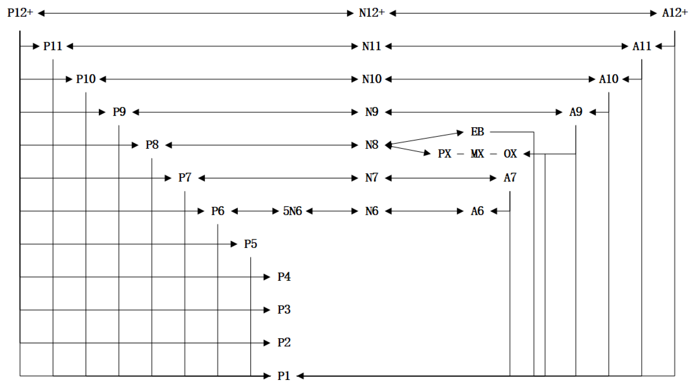
There are 34-component lumped including hydrogen. Although olefins account for a small proportion (about 1%) of the components involved in the reforming reaction, they are taken into account in order to consider the generality of the model. The lumped reaction network is shown in Figure 1.

The reaction network in Figure 1 includes 39 reforming reactions, including 7 dehydrogenation reactions of paraffins, 8 dehydrogenation reactions of naphthenes, 5 hydrolyzation reactions of aromatics, and 19 hydrocracking reactions of paraffins. The details are as follows:

Dehydrogenation reactions of paraffins:

$$P_i\leftrightarrow N_i+H_2,i=6\sim 12$$

(1)

Dehydrogenation reactions of naphthenes:

$$N_i\leftrightarrow A_i+3H_2,i=6\sim 12$$

(2)

Hydrolyzation reactions of aromatics:

$$\begin{array}{c}{A}_7+H_2\to A_6+P_1\hfill \\ A_8+H_2\to A_7+P_1\hfill \\ A_9+H_2\to A_8+P_1\hfill \\ A_{10}+H_2\to A_9+P_1\hfill \\ A_{11}+H_2\to A_{10}+P_1\hfill \end{array}$$

(3)

Hydrocracking reactions of paraffins:

$$\begin{array}{c}{P}_4+H_2\to P_2+P_2\\ P_5+H_2\to P_2+P_3\\ P_6+H_2\to P_i+P_{6-i},i=1,2,3\\ P_7+H_2\to P_i+P_{7-i},i=1,2,3\\ P_8+H_2\to P_i+P_{8-i},i=1,2,3,4\\ P_9+H_2\to P_i+P_{9-i},i=1,2,3,4\\ P_{10}+H_2\to 0.1P_1+0.1P_2+0.15P_3+0.2P_4+0.9P_5+0.2P_6\\ +0.15P_7+0.1P_8+0.1P_9\\ P_{11}+H_2\to 0.3P_2+0.25P_3+0.25P_4+0.2P_5+0.2P_6+0.25P_7+0.25P_8+0.3P_9\\ +0.25P_7+0.25P_8+0.3P_9\\ P_{12}+H_2\to 0.1P_1+0.15P_2+0.15P_3+0.15P_4+0.15P_5+0.6P_6\\ +0.15P_7+0.15P_8+0.15P_9+0.15P_{10}+0.1P_{11}\end{array}$$

(4)

2.2. Establishment of Reactor Model for Continuous Catalytic Reforming Process

In the continuous catalytic reforming process, the reforming reactor is the core device, so the reasonable modeling of the reforming reactor is the most critical in the whole process [14]. For the 34-component lumped reaction network established in this paper, the Hougen–Watson rate equation is used to describe it and 39 reaction rate equations can be obtained. The equations are as follows:

Dehydrogenation reactions of paraffins:

$$r_{j_z}=d{Y}_P/d(V_c/F_z)=k_{j_z}·(Y_P-Y_N/K_{ep{j}_z}),j_z=1\sim 7$$

(5)

Dehydrogenation reactions of naphthenes:

$$r_{j_z}=d{Y}_N/d(V_c/F_z)=k_{j_z}·(Y_N-Y_A/K_{ep{j}_z}),j_z=8\sim 15$$

(6)

Hydrolyzation reactions of aromatics:

$$r_{j_z}=d{Y}_A/d(V_c/F_z)=k_{j_z}·Y_A,j_z=16\sim 20$$

(7)

Hydrocracking reactions of paraffins:

$$r_{j_z}=d{Y}_P/d(V_c/F_z)=k_{j_z}·Y_P,j_z=21\sim 39$$

(8)

where $r_{j_z}$ is the reaction rate; Y is the molar flow rate of each lumped component; $Y_P$, $Y_N$, $Y_A$ are the molar flow rates of paraffins, naphthenes, and aromatics, respectively; $V_C$ is the catalyst loading; $F_z$ is the feed volume flow; $K_{ep{j}_z}$ is the $j_{\mathrm{z}}$-th reaction equilibrium constant; $k_{j_z}$ is the reaction rate constant—its expression is

$$k_{j_z}=k_{0j_z}·exp(-E_{j_z}/R_{q}T)·P_h^{b_{j_z}}·{\varphi }_{j_z}·{\mu }_{j_z},j_z=1\sim 39$$

(9)

where $k_{0j_z}$ is the reaction frequency factor; $E_{j_z}$, $b_{j_z}$ is the reaction activation energy and pressure index, respectively; $P_h$ is the hydrogen partial pressure in the reactants; $R_q$ is the molar gas constant; T is the reaction temperature; ${\varphi }_{j_z}$ is the catalyst activity factor; ${\mu }_{j_z}$ is the device factor.

In this paper, the radial structure of the reactor in the continuous catalytic reforming process is used, and combined with the principle of material balance and energy balance, the model equations of the reforming reactor can be obtained:

$$\left\{\begin{array}{c}\frac{d\stackrel{\rightharpoonup }{Y}}{dR}=\frac{2\pi RH}{LHSV·V_c}·\overrightarrow{\alpha }·\overrightarrow{r}\hfill \\ \frac{dT}{dR}=\frac{2\pi RH}{LHSV·V_c}\frac{\overrightarrow{r}·-\Delta \overrightarrow{H}}{{\overrightarrow{C}}_p·\overrightarrow{Y}}\hfill \end{array}\right.$$

(10)

where $\stackrel{\rightharpoonup }{Y}$ is the molar flow rate of 34—component lumped; R is the bed radius of radial reactor; H is the reactor height; LHSV = F_z/V_c is the liquid hour space velocity; $\stackrel{\rightharpoonup }{\alpha }$ is the stoichiometric coefficient matrix of each lumped component; $\Delta \stackrel{\rightharpoonup }{H}$ is the reaction heat vector; ${\stackrel{\rightharpoonup }{C}}_p$ is the constant pressure specific heat capacity vector; $\stackrel{\rightharpoonup }{r}=\stackrel{\rightharpoonup }{K}·\stackrel{\rightharpoonup }{Y}$ is the reaction rate vector of the reforming reaction, so the model equations of the reforming reactor can be rewritten as follows:

$$\left\{\begin{array}{c}\frac{d\stackrel{\rightharpoonup }{Y}}{dR}=\frac{2\pi RH}{LHSV·V_c}·\overrightarrow{\alpha }·\overrightarrow{K}·\overrightarrow{Y},\overrightarrow{Y}\left(R_0\right)={\overrightarrow{Y}}_0\hfill \\ \frac{dT}{dR}=\frac{2\pi RH}{LHSV·V_c}\frac{\overrightarrow{r}·-\Delta \overrightarrow{H}}{{\overrightarrow{C}}_p·\overrightarrow{Y}},T\left(R_0\right)=T_0\hfill \end{array}\right.$$

(11)

where $\overrightarrow{K}$ is the reaction rate constant matrix.

2.3. Property Calculation

The acquisition of some important physical property data is a prerequisite for model calculation, and the accuracy of these data has a great impact on the accuracy of the subsequent dynamic simulation. At the temperature of the continuous catalytic reforming reaction, all the reaction components are in a gaseous form. They can be regarded as ideal gas states and treated with the thermodynamic consistency equation [19]. In this paper, 5 calculation methods of important physical properties are given; the methods are as follows:

(1) Enthalpy

$$H_m=H=A+BT+C{T}^2+D{T}^3+E{T}^4+F{T}^5$$

(12)

where $H_m$ is the enthalpy of ideal gas at T; T is the reaction temperature; $A,B,C,D,E,F$ is the derived coefficient.

(2) Entropy

$$S=Bln\left(T\right)+2CT+\frac{3}{2}D{T}^2+\frac{4}{3}E{T}^3+\frac{5}{4}F{T}^4+G$$

(13)

where S is the entropy of an ideal gas at T; G is the derived coefficient.

(3) Constant pressure specific heat capacity

$${\overrightarrow{C}}_p=C_p=B+2CT+3D{T}^2+4E{T}^3+5F{T}^4$$

(14)

where $C_p$ is the heat capacity of ideal gas under constant pressure.

(4) Reaction heat

At the temperature of T, the formula is as follows:

$${\Delta }_r{H}_m^{\Theta }\left(T\right)=\sum \left(\alpha ·{\Delta }_f{H}_m^{\Theta }\left(298.15K\right)\right)+{\int }_{298.15K}^T\sum \left(\alpha ·C_p\left(T\right)\right)dT$$

(15)

where ${\Delta }_r{H}_m^{\Theta }$ represents the standard molar enthalpy of reaction; $\alpha$ is the stoichiometric coefficient; ${\Delta }_f{H}_m^{\Theta }$ represents the standard molar formation enthalpy; $C_p\left(T\right)$ represents the constant pressure specific heat capacity of each component at temperature T.

(5) Reaction equilibrium constant calculation For a reversible reaction $A_i\leftrightarrow A_j+n{H}_2$, the equilibrium constant at temperature T and a standard pressure of $100Kpa$ is

$$K_{ep}=K^{\Theta }\left(T\right)=exp(-{\Delta }_r{G}_m^{\Theta }\left(T\right)/RT)$$

(16)

where ${\Delta }_r{G}_m^{\Theta }$ is the Gibbs free energy of standard mole generation at temperature T, also known as the standard mole free enthalpy, and the calculation formula is

$${\Delta }_r{G}_m^{\Theta }\left(T\right)={\Delta }_r{H}_m^{\Theta }\left(T\right)-T·{\Delta }_r{S}_m^{\Theta }\left(T\right)$$

(17)

where ${\Delta }_r{H}_m^{\Theta }\left(T\right)$ knows that the calculation formula of standard molar entropy ${\Delta }_r{S}_m^{\Theta }\left(T\right)$ is

$${\Delta }_r{S}_m^{\Theta }\left(T\right)={\Delta }_r{S}_m^{\Theta }\left(298.15K\right)+{\int }_{298.15K}^T\frac{\sum \left(\alpha ·C_p\right)}{T}dT$$

(18)

${\Delta }_r{S}_m^{\Theta }\left(298.15K\right)$ is the standard molar entropy of the component in the standard state.

3. Simultaneous Method Based on Finite-Element Collocation

This paper belongs to the differential–algebraic optimization proposition that contains both differential equations and algebraic equations. The simultaneous method based on finite-element collocation is very suitable for solving this type of problem due to its unique advantages. This method has many advantages of the Runge–Kutta discrete method [20,21,22,23,24,25]. In this method, the differential state variable expression is as follows:

$$w\left(z\right)=w_{i_y-1}+h_{i_y}\sum _{q=1}^K{\Omega }_q\left(\frac{z-z_{i_y-1}}{h_{i_y}}\right)\frac{\mathrm{d}w}{\mathrm{d}{z}_{i_y,q}}$$

(19)

where $w_{i_y-1}$ represents the value at the initial position of the $i_y$-th finite element; $h_{i_y}$ represents the length of the finite element $i_y$, ${\Omega }_q\left(t\right)=\int {\displaystyle \prod _{r=1,r\ne q}^K}\frac{(\tau -{\rho }_r)}{({\rho }_q-{\rho }_r)}d\tau$; the conversion relationship between t and $\tau$ is $\tau ={\rho }_r+\frac{t-t_r}{h_{i_y}}$, and satisfies the polynomial of order K: $\begin{array}{c}{\Omega }_q\left(0\right)=0q=1\cdots ,K\hfill \\ {\Omega }_q^{\prime }\left({\rho }_r\right)=\left\{\begin{array}{c}1,q=r\hfill \\ 0,q\ne r\hfill \end{array}\right.(q,r=1,\cdots ,K)\hfill \end{array}$; here, z can represent space or time, ${\rho }_r$ is the position of the r-th configuration point in the finite element/the r-th root of the Radau equation, ${\rho }_q$ is the position of the q -th configuration point in the finite element/the q-th root of the Radau equation, $\mathrm{d}w/\mathrm{d}{z}_{i_y,q}$ refers to the first derivative at the configuration point q in the $i_y$-th finite element, and $t_r$ is the time corresponding to the r-th configuration point. The idea of the simultaneous method based on finite-element collocation is to uniformly discretize the entire time domain $[t_0,t_f]$ into $ne$ finite elements, and the entire time domain is divided into

$$t_0=t_0<t_1<t_2<\dots <t_{ne}=t_f$$

(20)

The length $h_i$ of each finite element can be expressed as follows:

$$h_{i_y}=(t_f-t_0)/ne,i_y=1,\cdots ,ne$$

(21)

The expressions of differential state variables, algebraic state variables, and control variables are as follows:

$$w_{i_y}=w_{i_y-1}+h_{i_y}\sum _{q=1}^K{\Omega }_q\left(1\right)\frac{\mathrm{d}w}{\mathrm{d}{z}_{i_y,q}}$$

(22)

$$y\left(z\right)=\sum _{q=1}^K{\psi }_q\left(\frac{z-z_{i_y-1}}{h_{i_y}}\right)y_{i_y,q}$$

(23)

$$u\left(z\right)=\sum _{q=1}^K{\psi }_q\left(\frac{z-z_{i_y-1}}{h_{i_y}}\right)u_{i_y,q}$$

(24)

where $y_{i_y,q}$ represents the value of the algebraic variable at the q-th configuration point at the $i_y$-th finite element, and $u_{i_y,q}$ represents the value of the control variable at the q-th configuration point at the $i_y$-th finite element. ${\psi }_q$ represents the Lagrange function of the q-th configuration point at the $i_y$-th finite element, and the expression is as follows:

$${\psi }_q\left(t\right)=\prod _{j_y=1}^K\frac{(t-t_{i_y,j_y})}{(t_q-t_{j_y})}=\prod _{j=1}^K\frac{(t-t_{i_y,j_y})/h_{i_y}}{({\rho }_q-{\rho }_{j_y})}$$

(25)

$${\psi }_q\left(t_{i_y,j_y}\right)=\left\{\begin{array}{c}1,q=j_y\hfill \\ 0,q\ne j_y\hfill \end{array}\right.(q,j_y=1,\dots ,K)$$

(26)

The configuration point of each finite element is K; the position corresponding to each configuration point is the root $[{\rho }_1,{\rho }_2,\dots ,{\rho }_K]$ of the orthogonal polynomial of the Radau configuration point; and the time corresponding to each configuration point is $t_{i_y,j_y}=t_{i_y-1}+h_{i_y}{\rho }_{j_y},j_y=1,\dots ,K$, where $t_{i_y,j_y}$ represents the initial time at the $j_y$-th configuration point of the $i_y$-th finite element.

$${\psi }_q\left(t\right)=\prod _{r=1,r\ne q}^K\frac{(t-t_r)/h_{i_y}}{({\rho }_q-{\rho }_r)}=\prod _{r=1,r\ne q}^K\frac{(\tau -{\rho }_r)}{({\rho }_q-{\rho }_r)}$$

(27)

When ${\Omega }_q\left(0\right)=0q=1\dots ,3$, then

$$\begin{array}{c}{\Omega }_1\left(t\right)=\int \frac{(\tau -{\rho }_2)}{({\rho }_1-{\rho }_2)}\frac{(\tau -{\rho }_3)}{({\rho }_1-{\rho }_3)}d\tau \hfill \\ {\Omega }_2\left(t\right)=\int \frac{(\tau -{\rho }_1)}{({\rho }_2-{\rho }_1)}\frac{(\tau -{\rho }_3)}{({\rho }_2-{\rho }_3)}d\tau \hfill \\ {\Omega }_3\left(t\right)=\int \frac{(\tau -{\rho }_1)}{({\rho }_3-{\rho }_1)}\frac{(\tau -{\rho }_2)}{({\rho }_3-{\rho }_2)}d\tau \hfill \end{array}Z$$

(28)

As the differential state variable has continuity, it means that the final value of the current finite element differential state variable is equal to the initial value of the next finite element differential state variable. The expression is as follows:

$$w_{i_y+1,0}=w_{i_y,0}+h_{i_y}\sum _{q=1}^K{\Omega }_q\left(1\right)\frac{dw}{d{z}_{i_y,q}}$$

(29)

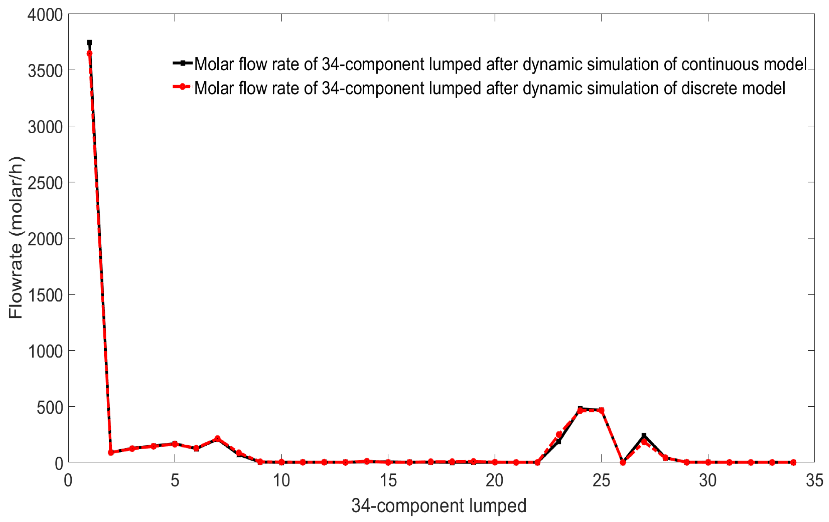
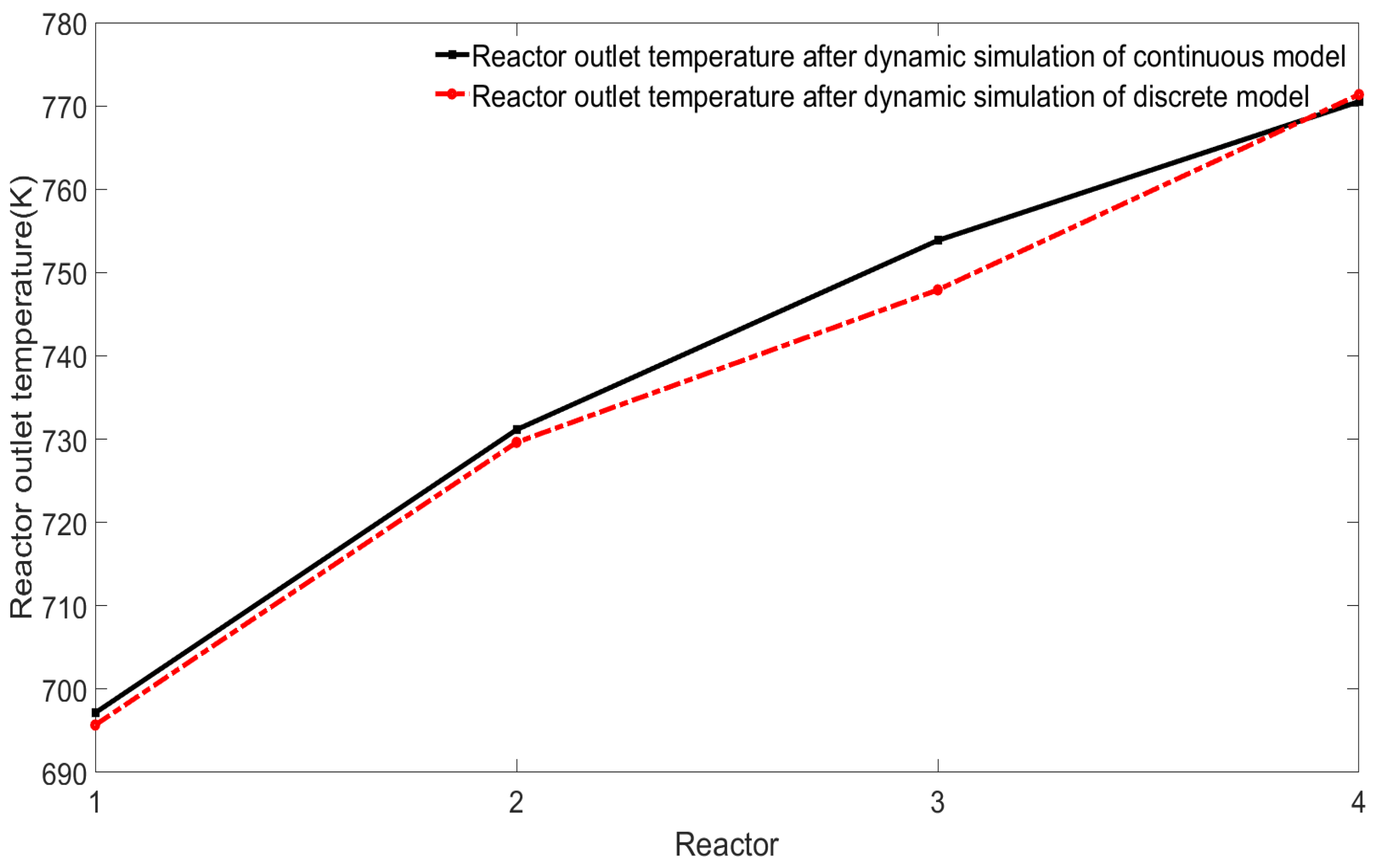
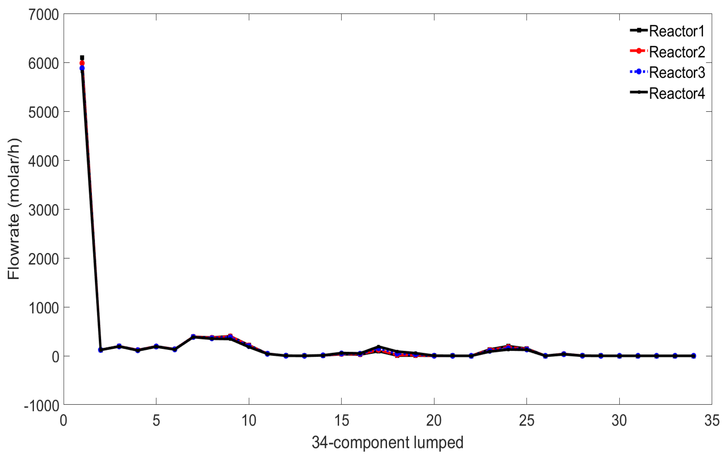
After the mechanism model of the continuous catalytic reforming process is discretized by a simultaneous method based on finite-element collocation, many discrete variables and algebraic equations will be obtained, so that the nonlinear solver can be used to dynamically simulate the system. Since this method has many advantages of the Runge–Kutta discrete method, and the Runge–Kutta discrete method has high discrete accuracy, the dynamic simulation of the discrete model and the dynamic simulation of its own continuous model will have a very high consistency. Comparison and verification will be conducted in the following model verification phase.

4. Parameter Estimation and Model Verification

4.1. Parameter Estimation

After the model is discretized by the simultaneous method based on finite-element collocation, in order to make the model consistent with the actual production process, it is necessary to use parameter estimation methods to correct the model. In this paper, the interior point algorithm is used to estimate the parameters of the pre-exponential factor of reaction and the device performance coefficient. The principle of the interior point algorithm is as follows:

Set the parameter vector x to be estimated, x is expressed as the pre-exponential factor of the reaction and the device performance coefficient, and the constrained optimization problem can be set as

$$\begin{array}{c}minG\left(x\right)\hfill \\ s.t.c\left(x\right)=0\hfill \\ x\ge 0\hfill \end{array}$$

(30)

Among them, $G\left(x\right)$ is the objective function and $c\left(x\right)$ is the equality constraint including the differential equations and physical property equations mentioned in the mechanism modeling part, and is a nonlinear equation group, which expresses the relationship between process variables. Its Lagrange function is defined as

$$L(x,\lambda ,v)=G\left(x\right)+c{\left(x\right)}^T\lambda -x^{T}v$$

(31)

where $\lambda$ and v are the Lagrange multipliers of the equality constraint and boundary constraint, respectively.

For the optimization problem of Equation (30), the barrier method is used to add boundary constraints to the objective function in the form of barrier terms [26], so Equation (30) can be transformed into

$$\begin{array}{c}min{\phi }_{\mu }(x)=G(x)-\mu {\displaystyle \sum _{i=1}^n}ln\left(x^{\left(i\right)}\right)\hfill \\ s.t.c\left(x\right)=0\hfill \end{array}$$

(32)

where $\mu >0$ is the obstacle parameter and ${\phi }_{\mu }\left(x\right)$ is the obstacle function. When x is close to the boundary, the value of the objective function can be infinite, so the solution of this problem will be inside the boundary area.

For the solution of Equation (32), it is necessary to consider the first-order necessary condition of its local optimum—that is, the KKT (Karush–Kuhn–Tucker) condition is

$$\begin{array}{c}\nabla G\left(x\right)+A\left(x\right)\lambda -v=0\hfill \\ c\left(x\right)=0\hfill \\ Xv-\mu e=0\hfill \\ x^{\left(i\right)}\ge 0\hfill \\ \frac{\mu }{x^{\left(i\right)}}\ge 0\hfill \end{array}$$

(33)

where $\nabla G$ is the gradient vector, $A\left(x\right)=\nabla c\left(x\right)$ is the transpose of the constrained Jacobian matrix, X is the diagonal matrix obtained by taking the vector x as the diagonal element, and e is the vector whose elements are all 1.

Since formula (32) satisfies the KKT condition, Newton’s method can be applied to formula (32) [27], the search direction at the iteration point is

$$\left[\begin{array}{cc}{W}_k& A_k\\ A_k^T& 0\end{array}\right]\left[\begin{array}{c}{d}_k\\ {\lambda }_{k+1}\end{array}\right]=-\left[\begin{array}{c}{g}_k\hfill \\ c_k\hfill \end{array}\right]$$

(34)

where $W_k$ is the Hessian matrix and $g_k$ is the gradient vector.

Newton’s method requires the calculation of the second-order derivative to form the true Hessian matrix, which may be nonpositive definite, so this paper uses the BFGS method to replace the Newton method. The BFGS method constructs a matrix that does not contain the second-order partial derivative to approximate the inverse matrix of the Hessian matrix in Newton’s method, so as to overcome the defects of Newton’s method [28]. In order to construct this matrix, we use Taylor’s formula to expand $\nabla G\left(x\right)$ at $x_{k+1}$ and evaluate it:

$$\nabla G\left(x_{k+1}\right)-\nabla G\left(x_k\right)\approx {\nabla }^{2}G\left(x_{k+1}\right)(x_{k+1}-x_k)$$

(35)

Let $s_k=x_{k+1}-x_k$, $y_k=\nabla G\left(x_{k+1}\right)-\nabla G\left(x_k\right)$, $B_{k+1}={\nabla }^{2}G\left(x_{k+1}\right)$, so Formula (35) can be modified as

$$B_{k+1}{s}_k=y_k$$

(36)

where $B_{k+1}$ is the approximation matrix constructed for the Hessian matrix.

When the above steps are completed, $B_k$ also needs to be corrected. The correction formula is as follows:

$$B_{k+1}=B_k-\frac{B_k{s}_k{\left(s_k\right)}^T{B}_k}{{\left(s_k\right)}^T{B}_k{s}_k}+\frac{y_k{\left(y_k\right)}^T}{{\left(y_k\right)}^T{s}_k}$$

(37)

The approximate matrix of the inverse matrix of the Hessian matrix is $H_k$, $H_k=B_k^{-1}$, so the correction formula of $H_k$ can be obtained:

$$H_{k+1}=V_k^T{H}_k{V}_k+{\zeta }_k{s}_k{s}_k^T$$

(38)

where ${\zeta }_k=1/y_k^T{s}_k$, $V_k=I-{\zeta }_k{y}_k{s}_k^T$.

In order to ensure global convergence, the interior point algorithm needs to perform a linear search along the search direction $d^{\left(k\right)}$. After the search, a search step size ${\alpha }_k$ can be obtained. After the search step size is obtained, the algorithm can obtain the next iteration point by formula (39):

$$x^{(k+1)}=x^{\left(k\right)}+{\alpha }_k{d}^{\left(k\right)}$$

(39)

4.2. Efficient Solution Strategy

The interior point algorithm used in this paper is based on the derivative information used to solve it, but the derivative information is time-consuming and the Jacobian matrix has very high sparsity; thus, this leads to the problem of too long a time to solve the derivative. As shown in Figure 2, when obtaining the derivative information of the parameter estimation method, two aspects can be considered: One is the objective function; this paper uses an analytical method to obtain its derivative information. The other is the constraint equation; this paper uses the method of differencing the constraint equation to obtain the sparse matrix, and derivation of the sparse matrix to obtain the sparse Jacobian Matrix to complete the acquisition of derivative information. The sparse Jacobian matrix obtained by the above method can be used to replace the original Jacobian matrix so that the problem of too long a solving time of the derivative can be resolved, thereby speeding up the solution.

In addition, the BFGS method used in the interior point algorithm needs to store the matrix during the calculation process. The problem solved in this paper is a large-scale optimization problem, and the obtained Hessian matrix has 7056 * 7056. The memory required for normal calculation of this problem is more than 10 times that of the Hessian matrix. In this case, dozens of GB of memory cannot be solved, which may lead to a memory crash. To solve this problem, this paper adopts the BFGS method with limited storage. This is because the BFGS method with limited storage does not generate the approximate matrix of the inverse matrix of the Hessian matrix, but stores $\omega$ pairs of curvature information $\{s_z,y_z\}$, and $H_k$ can be defined by the obtained curvature information [29,30,31,32], At the iteration point $x_k$, the initial matrix $H_0$ and $\omega$ curvature information pairs $\{s_z,y_z\}$ are given, $z=0,\cdots ,\omega -1$, where $\omega =min(k,\omega )$; in the $k+1$-th iteration, $H_k$ is updated with the BFGS method. The updated formula is

$$\begin{array}{c}{H}_{k+1}=(V_k^T\cdots V_{k-\omega }^T)H_0(V_{k-\omega }\cdots V_k)\hfill \\ +{\zeta }_{k-\omega }(V_k^T\cdots V_{k-\omega +1}^T)s_{k-\omega }{s}_{k-\omega }^T(V_{k-\omega +1}\cdots V_k)\hfill \\ +{\zeta }_{k-\omega +1}(V_k^T\cdots V_{k-\omega +2}^T)s_{k-\omega +1}{s}_{k-\omega +1}^T(V_{k-\omega +2}^T\cdots V_k^T)+\hfill \\ ⋮\hfill \\ +{\zeta }_k{s}_k{s}_k^T\hfill \end{array}$$

(40)

According to our numerical experiments, only the $\omega$ values in the range of 5∼9 can lead to good performance. The BFGS method with limited storage eliminates the need to store the matrix, which greatly saves space and prevents the problem of excessive memory.

4.3. Comparison between Simultaneous Method and Sequential Method

The dynamic simulation mainly includes two methods, namely, sequential method and simultaneous equations method. This paper takes the MATLAB platform as an example. The sequential method and simultaneous equations method are used on the MATLAB platform to dynamically simulate the mechanism model established in this paper. Figure 3 and Figure 4 show the time taken for part of the procedure for dynamic simulation using sequential method and simultaneous equations method.

It can be seen from Figure 3 and Figure 4 that in the comparison of the main program Calibration, the total time used for the simultaneous equations method is 50.735 s, while the total time used by the sequential method is 1269.877 s, which is approximately 25 times the total time for the simultaneous equations method. The reason for the difference in time is that the sequential method has a very large number of iteration nests, which take a lot of time. This comparison result clearly shows the superiority of the simultaneous equations method, which is the reason why this paper adopts the simultaneous equations method.

4.4. Model Verification

After the mechanism model of the continuous catalytic reforming process is discretized by a simultaneous method based on finite-element collocation, many discrete variables and algebraic equations are obtained. In order to verify the accuracy of the discrete model, some results of dynamic simulation of the discrete model and its own continuous model are compared in this paper.

Figure 5 shows the comparison of the change of the molar flow rate of 34-component lumped at the outlet of the final reactor after the dynamic simulation of the discrete model and its own continuous model, and Figure 6 shows the comparison of the outlet temperature of each reactor after the dynamic simulation of the discrete model and its own continuous model. It can be seen from these two figures that the difference between the results of the discrete model and its own continuous model is small.

In this paper, the internal state of the reactor is also dynamically simulated to further verify the accuracy of the discrete model. The discrete model and its own continuous model were used to dynamically simulate the temperature inside the reactor from the outside to the inside diameter. The results are shown in

Table 1. The distribution of reactor temperature after dynamic simulation of the continuous model.

		Reactor	1	2	3	4
	Temperature
Internal Location
14.29%R			799.450	798.050	796.050	803.250
28.57%R			727.155	760.798	774.127	789.055
42.86%R			713.115	747.765	763.432	781.736
57.14%R			705.826	740.430	757.175	777.483
71.43%R			701.344	735.759	753.164	774.796
85.71%R			698.445	732.682	750.521	773.049
100%R			696.610	730.713	748.833	771.945

and

Table 2. Discrete model dynamic simulation of reactor temperature distribution.

		Reactor	1	2	3	4
	Temperature
Internal Location
14.29%R			799.450	798.050	796.050	803.250
28.57%R			727.771	760.780	774.151	789.080
42.86%R			713.421	747.756	763.457	781.756
57.14%R			706.029	740.427	757.201	777.505
71.43%R			701.500	735.760	753.191	774.819
85.71%R			698.576	732.686	750.549	773.073
100%R			696.726	730.718	748.861	771.970

, where R is the bed radius of radial reactor.

It can be seen from Table 1 and Table 2 that the temperature distribution in the four reactors after the continuous model dynamic simulation is very close to the results obtained from the discrete model dynamic simulation.

From the above results, it can be concluded that the discrete method used in this paper is feasible and reasonable.

5. Dynamic Simulation in Different Situations

5.1. Dynamic Simulation under Different Input Parameters

After the mechanism model is established, the lumped components at the outlet of each reactor and the changes in the internal temperature of the reactor can be observed, and the influence of these parameters on the reactor can be observed by modifying the values of some parameters.

First, observe the change of the lumped components at the outlet of each reactor. The consumption of each lumped component can be seen from Figure 7.

As it is a 34-component lumped reaction, in order to make the results look simple, the lumped is simplified into five parts: H (hydrogen), P (paraffins), N (naphthenes), A (aromatics), C5 (carbon 5 and below). The actual molar masses of these five lumps can be obtained from the factory as 3743.435, 282.211, 14.228, 1411.125, and 646.046.

First of all, the effect of catalyst loading on each lumped component can be observed by proportionally increasing the catalyst loading. The results are shown in

Table 3. Units for Magnetic Properties and the effect of catalyst loading on each lumped component.

Lumped Components	Catalyst Loading Times
	1.25	1.5	1.75	2
H	6092.978	5984.619	5881.689	5809.893
P	1424.580	1408.033	1365.177	1301.799
N	176.421	237.919	334.1817	448.134
A	514.928	471.747	420.920	373.312
C5	762.195	757.556	750.861	743.211

.

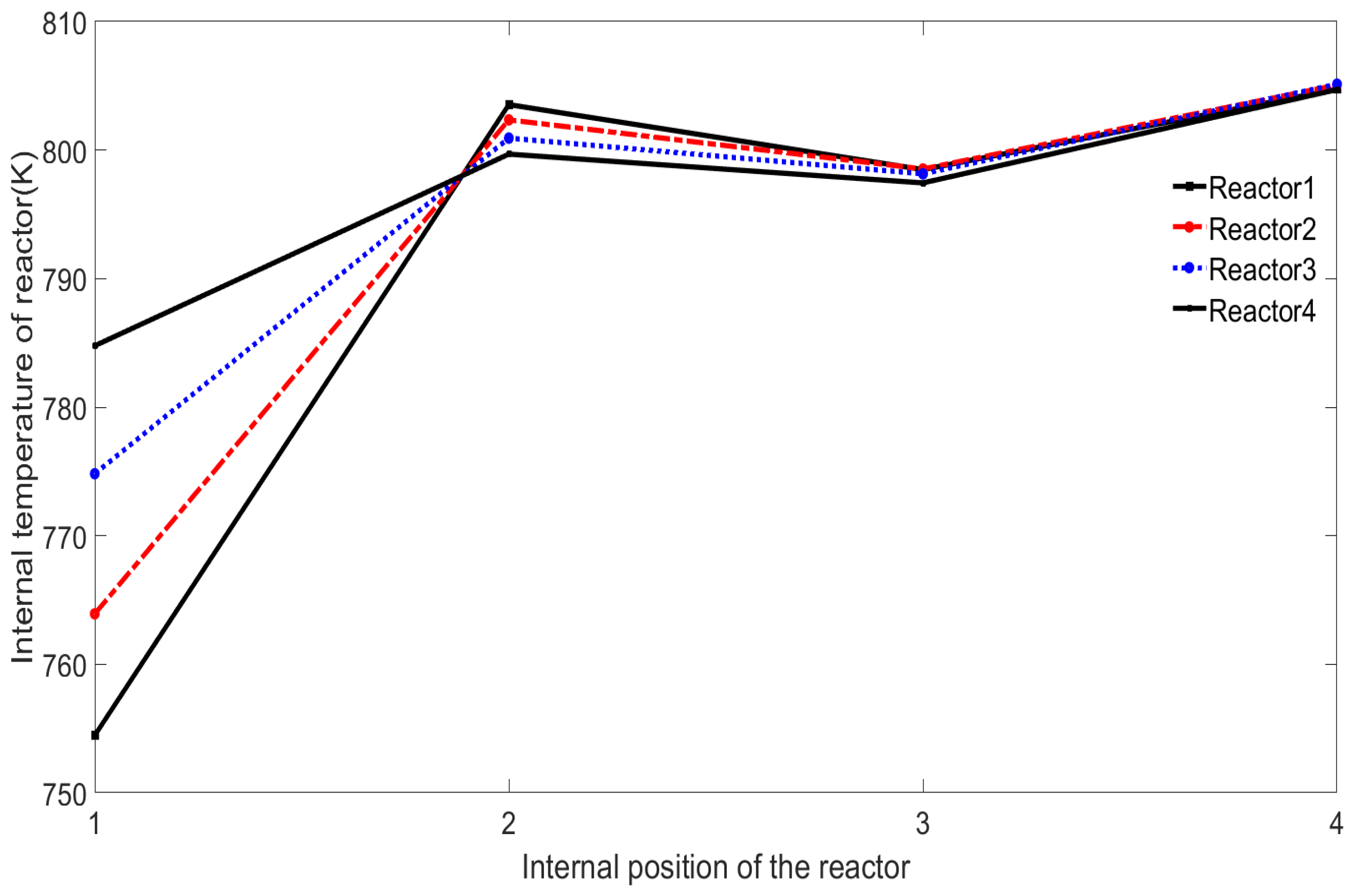
Secondly, observe the changes in the internal temperature of each reactor. As shown in Figure 8, the inside of each reactor is again divided into four parts for observation.

It can be seen from Table 3 that with the proportional increase in the catalyst loading, the contents of these five components all show a downward trend.

Secondly, by increasing the input temperature of the reactor proportionally, the influence of the input temperature of the reactor on each lumped component can be observed. The results are shown in

Table 4. The influence of reactor input temperature on each lumped component.

Lumped Components	Input Temperature Multiple
	1.25	1.5	1.75	2
H	5909.392	5867.337	5932.714	6233.389
P	1395.379	1373.219	1404.260	1422.319
N	293.547	339.434	272.553	124.489
A	436.161	413.677	447.534	564.738
C5	738.678	735.443	740.596	773.474

.

It can be seen from Table 4 that as the reactor temperature increases proportionally, most of these five components show a downward trend. However, when the temperature is too high—for example, when the reactor temperature ratio increases to 1.75 times—A and C5 no longer decrease but increase, which means that the temperature is too high and some reversible reactions may occur, which is obviously not the desired result, so the temperature needs to be controlled below a reasonable range.

5.2. Sensitivity Analysis

In this paper, the sensitivity of the yield of each product was analyzed by modifying the temperature and hydrogen oil ratio. As the $C_{5+}$ liquid yield, aromatics yield, and octane number are more important than for other products, these three products are mainly analyzed in this paper.

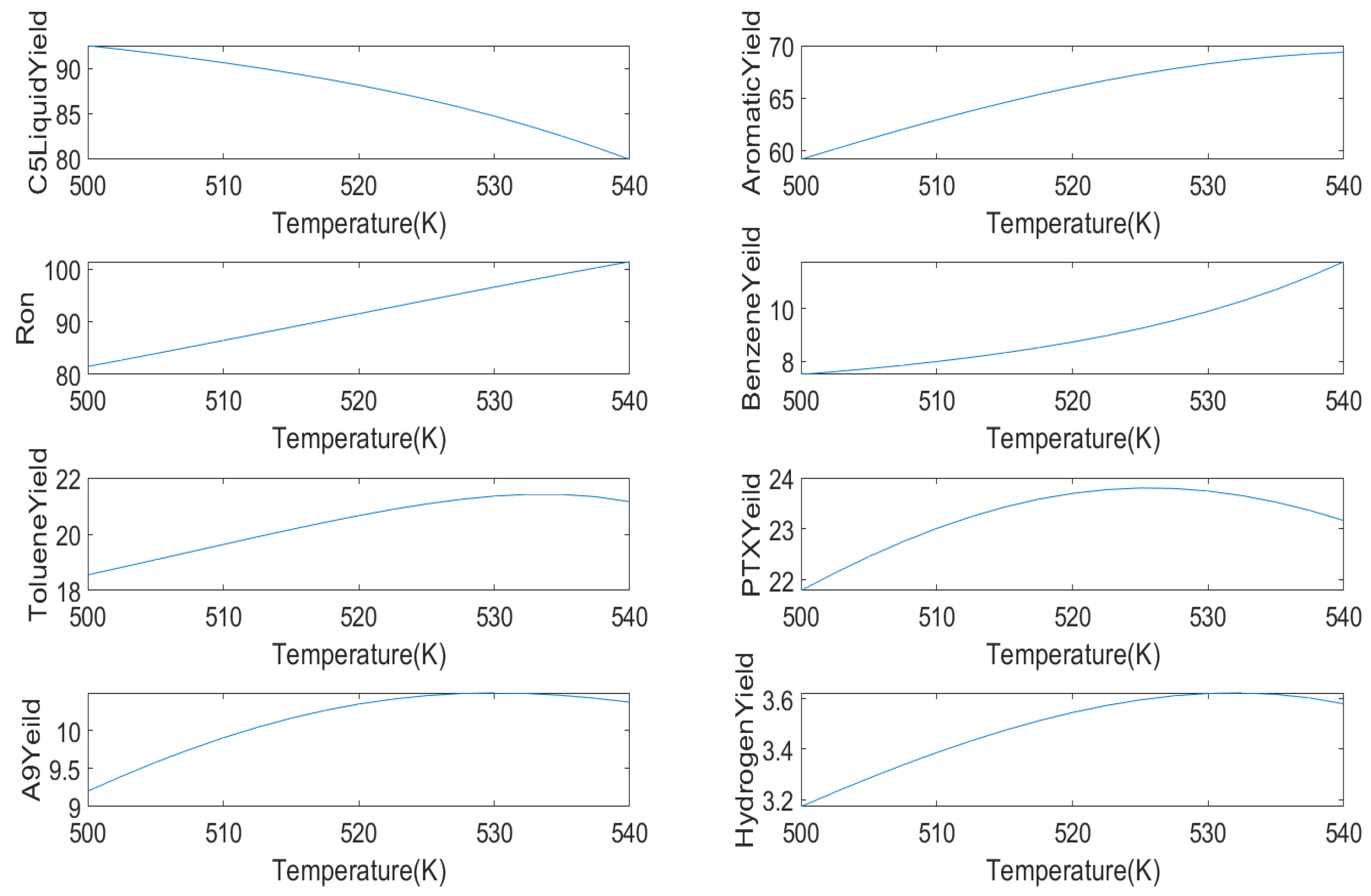
The first is the influence of temperature on $C_{5+}$ liquid yield, aromatic yield, benzene yield, toluene yield, mixed xylene yield, C9 aromatics yield, hydrogen yield, and octane number, as shown in Figure 9.

In industry, the reaction temperature is generally set to 480∼530 °C; this article sets the reaction temperature to 500∼540 °C on this basis. With the increase in the reaction temperature, the yield of aromatics and octane number also increase. When the temperature reaches 530 °C, the yield of aromatics tends to be flat. At this time, the yield of aromatics is between 72 and 74 (wt%). This is because the cycloalkane dehydrogenation reaction is a strong endothermic reaction, and higher temperature will increase the aromatics yield. However, when the temperature is too high, the alkane hydrocracking reaction will exceed the cycloalkane dehydrogenation reaction rate, so the aromatics yield will decrease. The liquid yield of $C_{5+}$ decreases with the increase in the reaction temperature, which is approximately a linear relationship. When the reaction temperature is higher than 510 °C, a lower liquid yield will be obtained.

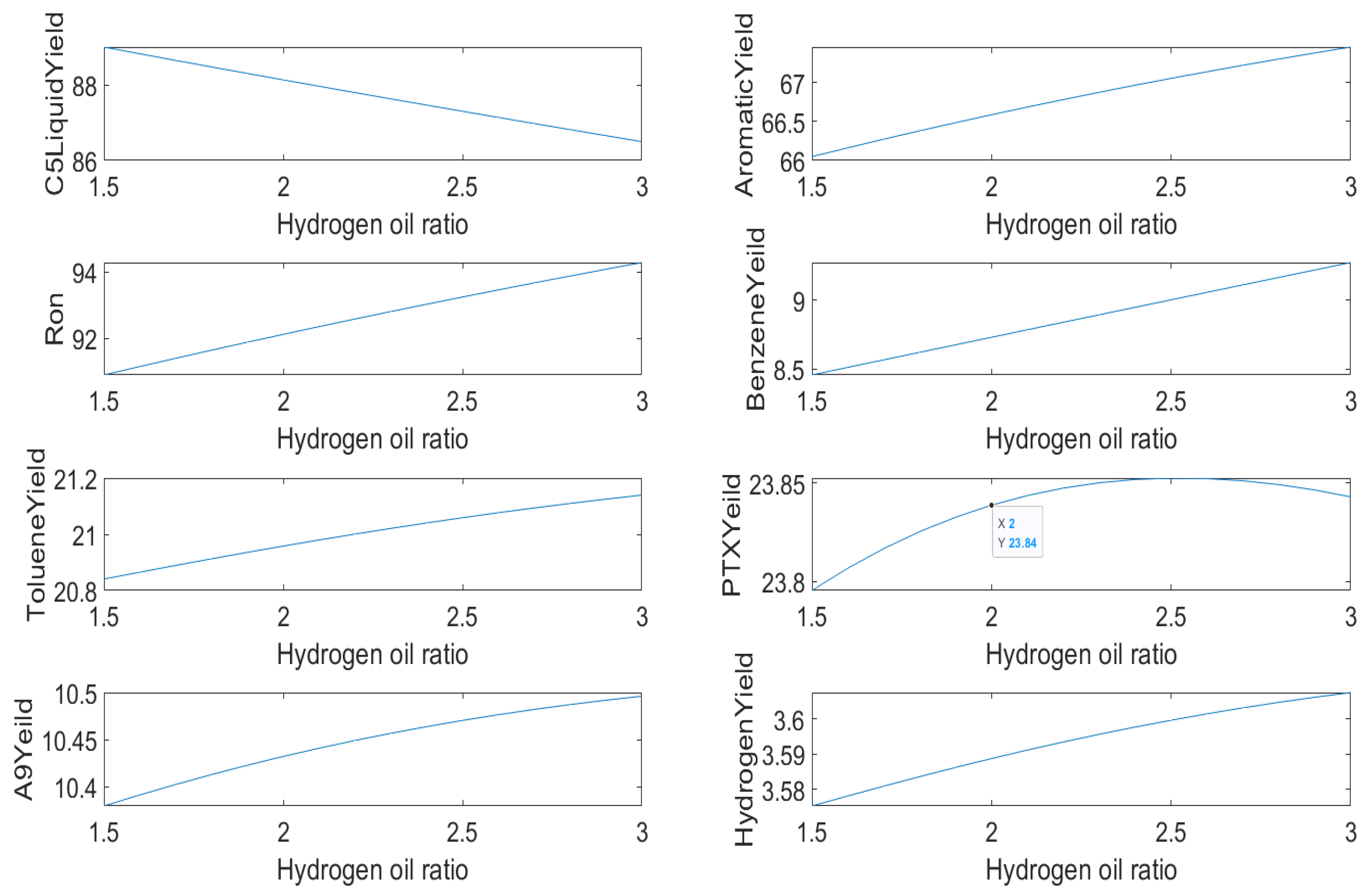
The second is the influence of hydrogen–oil ratio on $C_{5+}$ liquid yield, aromatic yield, benzene yield, toluene yield, mixed xylene yield, C9 aromatics yield, hydrogen yield, and octane number, as shown in Figure 10.

With the increase in hydrogen–oil ratio, the catalyst activity can be improved, which is conducive to improve the yield of aromatics and octane number. At the same time, the increase in hydrogen–oil ratio will also accelerate the reaction rate of alkane hydrocracking and aromatics hydrocracking, and reduce the yield of $C_{5+}$ liquid.

From the sensitivity analysis, we can discover the influence of temperature and hydrogen–oil ratio on the yield of each product. These results can also be compared with the actual situation to verify the accuracy of the model, and it can also pave the way for subsequent optimization solutions.

6. Conclusions

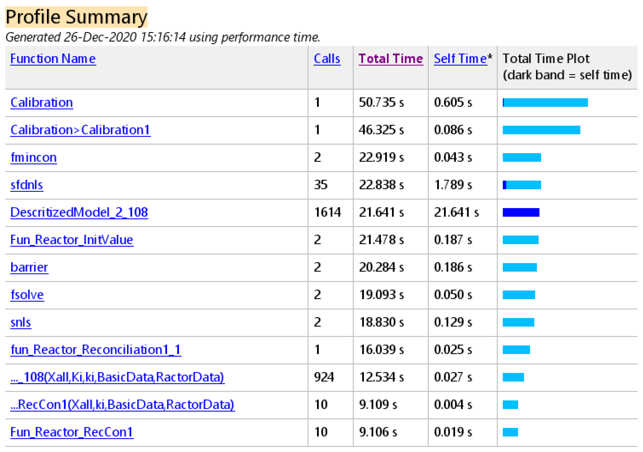
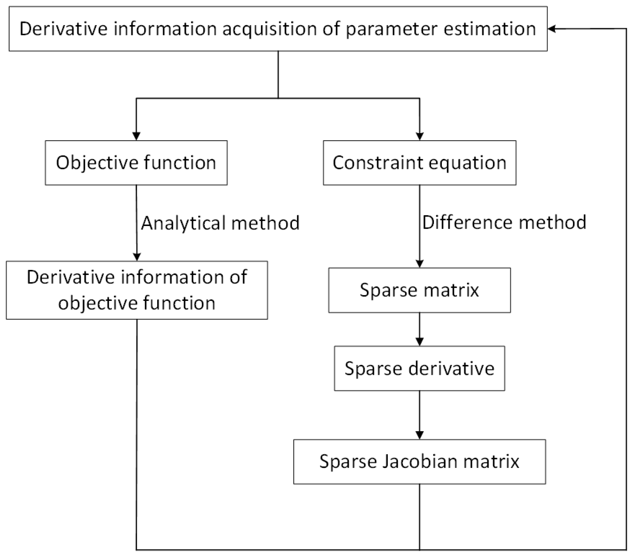
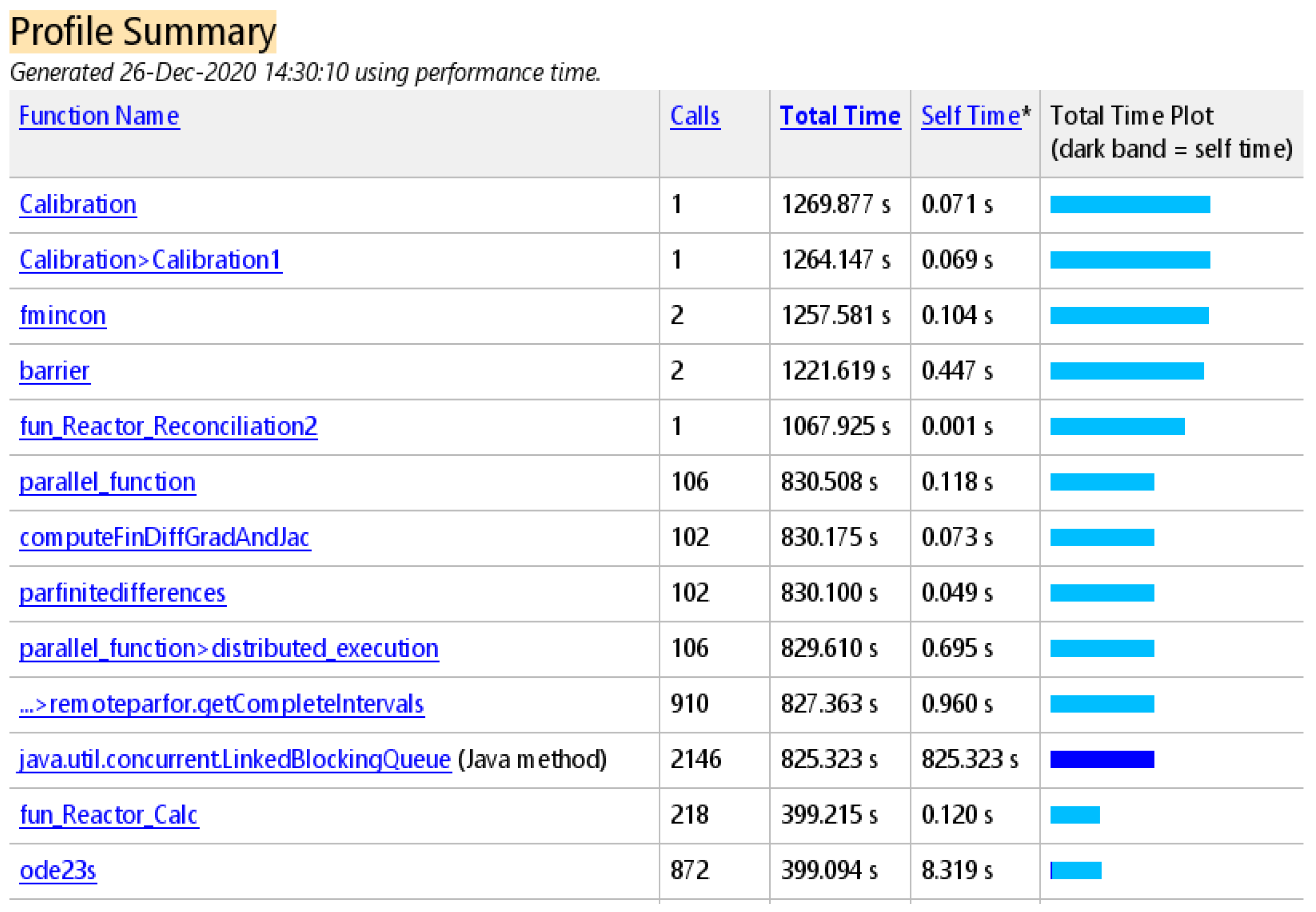
Based on the basic principles of reforming kinetics, thermodynamics, material balance, energy balance, etc., a 34-lumped mechanism model described by differential algebra is established in this paper. The differential equations are discretized through the simultaneous equations method of finite-element collocation to transform them into large-scale nonlinear programming problems, so as to solve and simulate the mechanism model consisting of 144 differential equations and several algebraic equations, and adopt the internal point algorithm for parameter estimation and model verification. In order to avoid the problem of too long a derivative solution time and too large memory in the solution process, methods such as sparse derivative and limited storage BFGS are used. In the model verification, taking the MATLAB platform as an example, the sequential method and the simultaneous equations method were used on the MATLAB platform to dynamically simulate the mechanism model established in this paper. It can be seen from the results that the time taken by the sequential method is about 25 times the time taken by the simultaneous equations method. Finally, based on the model verification, the catalyst loading amount and reactor input temperature are to observe its impact on each reactor, and then observe the impact on each component through the proportional increase in catalyst loading and reactor input temperature. The above process is to conduct dynamic simulation and sensitivity analysis of the whole process by modifying different input parameters. In addition, sensitivity analysis can verify the accuracy of the model and pave the way for subsequent optimization solutions. The results show that the mechanism model given in this paper is in line with the actual situation in our country and the solution method proposed can quickly and accurately simulate the continuous catalytic reforming process.