Abstract
One of the influential models in the artificial neural network (ANN) research field for addressing the issue of knowledge in the non-systematic logical rule is Random k Satisfiability. In this context, knowledge structure representation is also the potential application of Random k Satisfiability. Despite many attempts to represent logical rules in a non-systematic structure, previous studies have failed to consider higher-order logical rules. As the amount of information in the logical rule increases, the proposed network is unable to proceed to the retrieval phase, where the behavior of the Random Satisfiability can be observed. This study approaches these issues by proposing higher-order Random k Satisfiability for k ≤ 3 in the Hopfield Neural Network (HNN). In this regard, introducing the 3 Satisfiability logical rule to the existing network increases the synaptic weight dimensions in Lyapunov’s energy function and local field. In this study, we proposed an Election Algorithm (EA) to optimize the learning phase of HNN to compensate for the high computational complexity during the learning phase. This research extensively evaluates the proposed model using various performance metrics. The main findings of this research indicated the compatibility and performance of Random 3 Satisfiability logical representation during the learning and retrieval phase via EA with HNN in terms of error evaluations, energy analysis, similarity indices, and variability measures. The results also emphasized that the proposed Random 3 Satisfiability representation incorporates with EA in HNN is capable to optimize the learning and retrieval phase as compared to the conventional model, which deployed Exhaustive Search (ES).
1. Introduction
A hallmark of any Artificial Neural Network (ANN) is the ability to behave according to the pre-determined output or decision. Without an “optimal” behavior, ANN will result in producing random outputs or decisions, which leads to useless information modelling. Although, ANNs can learn and model complex relationships, which is important to represent real-life problems, it lacks the interpretability of the results obtained and approximated. There is no simple correlation between the strength of the connection between neurons (the weights) and the results being approximated. Understanding the relationship between the ANN structure and the behavior of the output is a major goal in the field of Artificial Intelligence (AI). One of the notable ANN that has an association feature form of learning model is Hopfield Neural Network (HNN) [1]. The information is stored in the form bipolar representation and connected by synaptic weight. After the introduction of HNN, this network has been modified vigorously to solve optimization problems [1], medical diagnosis [2,3,4], electric power sector [5], investment [6], and many more. Despite achieving extraordinary development in various performance metrics for any given problem, the optimal structure of HNN is still debatable among the ANN practitioners. To this end, the choice of the most optimal symbolic structure that governs HNN must be given fair share of attention.
The satisfiability (SAT) logical rule has a simple and flexible structure to represent the real-world problems. Satisfiability (SAT) is an NP-complete problem that was proven by [7] and plays a fundamental role in computational complexity theory [8,9,10]. One of the potential applications for SAT is the logical representation of the ANN. The goal of the logical representation is to represent the dataset and later filtered by the optimal logical rule. An interesting study conducted by [11] emphasized the complementary relationship between the logic and ANN in the field of AI. According to this study, computational logic is well-suited to represent structured objects and structure-sensitive processes for rational agents, while the ability to learn and to adapt to new environments is met by ANNs. One of the earliest efforts in implementing the logical rule in ANN was proposed by [12]. This work was inspired by the equivalence of the symmetrical mapping between the propositional logical rule with the energy function of the ANN [13,14]. After the emergence of logical rule in ANN, several logical rules have been proposed. The work by [15] proposed a higher-order Horn Satisfiability in Radial Basis Function Neural Network (RBFNN). The proposed work has been extended to another variant of logical rule namely 2 Satisfiability (2SAT) [16]. In this work, 2SAT became a logical structure to determine the parameters involved in RBFNN, thus fixing the number of hidden layers. The result from the performance evaluation in this work demonstrates the effectiveness of 2SAT in governing the structure of RBFNN. The first non-satisfiable logical rule namely Maximum k Satisfiability (MAXkSAT) in HNN was introduced by [17]. Despite achieving non-zero cost function during learning phase, the results showed a solid performance of the proposed model in obtaining global minimum energy and the highest value of the ratio of satisfied clause. Unfortunately, the mentioned studies focused on using the systematic logical rule where the number of variables in each clause is always constant. The prospect of the non-systematic logical rule in ANN is still poorly understood.
One of the challenges in embedding logical rule in HNN is the effectiveness of the learning phase. Output of the final state in HNN is structure-dependent and requires effective learning mechanism. Despite obtaining the optimal final state in previous studies such as in [17], finding logical assignments that lead to the optimal value of the cost function becomes convoluted as the number of logical clause increase. This is due to the probability of finding that the optimal cost function value of the HNN will reduce to zero. As a result, the final state of HNN governed by logical rule will be trapped into local minimum energy or suboptimal state. For instance, the work of [18] demonstrates the main weaknesses of conventional HNN in terms of retrieval capacity as the number of neurons increases. To overcome this issue, utilizing metaheuristic algorithm to find the optimal neuron assignment that leads to the minimization of the cost function has been proposed. [19] proposed Genetic Algorithm (GA) in learning 2SAT logical rule in HNN. The proposed metaheuristics is reported to obtain the optimal final state that corresponds to absolute minimum energy of the logical rule. The final state of the neuron exhibits higher value of global minima ratio, lower hamming distance and lower computational time. Ref. [20] proposed Artificial Immune System (AIS) to complement 3 Satisfiability (3SAT) in Elliot based HNN. The proposed method has been compared with other conventional metaheuristics algorithm such as Exhaustive Search (ES) and GA. The use of metaheuristics was extended to another logical variant that is not satisfiability. Ref. [21] proposed an interesting comparison among the prominent metaheuristics in learning Maximum 2 Satisfiability (MAX2SAT) logical rule. In this study, Artificial Bee Colony (ABC) integrated with MAX2SAT is observed to outperform other major metaheuristics. Despite the possibility of overfitting during learning phase of HNN, ABC remains competitive in finding the optimal assignment that minimizes the cost function of the MAX2SAT. In another development, [22] proposed Imperialist Competitive Algorithm (ICA) to optimize 3 Satisfiability (3SAT) in HNN. The proposed method was implemented in logic mining paradigm where the proposed ICA is reported to optimize the logical extraction of the benchmark datasets. However, all the mentioned metaheuristics algorithms only learn systematic logical rule (either systematic second order or third-order logical rule). The proposed metaheuristics only discover single search space and no effective solution partitioning to locate the alternative neuron assignment that minimizes the cost function.
Currently, Election Algorithm (EA) proposed by [23] starts to gain popularity in solving various optimization problems. EA is inspired by the social behavior of individuals during electoral activity. EA simulates the actual political electoral systems that are organized by governments such as presidential election that starts with grouping the population into parties and selecting a representative of each party to convey their beliefs and ideas to the public. Parties compete against each other for seeking the most votes and the candidate who gets the most votes will be the leader. This strategy has a good resemblance to other papers which utilizes candidate as their potential solution of the objective function. In [24], the authors introduced Election Campaign Optimization (ECO) algorithm by considering the solution of the function as a candidate. In this case, the higher prestige of a particular candidate, the larger the cover range that results in smaller mean square deviation. Another resemblance of EA is reported in Evolutive Election Based Optimization (EVEBO) [25]. EVEBO is reported to utilize different types of electoral system to conduct series of optimization effort for both combinatorial and numerical problems. For this reason, EVEBO has more degree of freedom to be applied for a wide range of problems. Emami later proposed [26] the Chaotic Election Algorithms (CEA) by introducing migration operator to complement the existing EA. CEA enhances the EA by implementing chaotic positive advertisement to accelerate the convergence because the distance function that is used to find the eligibility consumes more computation time. In the development of logic programming in HNN, [27] has successfully implemented the first non-systematic logical rule namely Random 2 Satisfiability (RAN2SAT) in HNN. The proposed work utilized EA to find the correct assignment that leads to minimize the cost function. The proposed EA in this work was inspired by the work of [23] where there were three operators have been introduced to optimize the learning phase of HNN for RAN2SAT. They adopt an interesting distance function to complement the structure of RAN2SAT. The proposed method can perform the learning phase with minimal error and result in high retrieval capacity. However, despite their great potential, the computational ability of EA in doing higher order Random k Satisfiability (RANkSAT) has not been demonstrated. Higher order RANkSAT creates both upsides and downsides during learning phase of HNN. Third order logic in RANkSAT for (RAN3SAT) can be easily satisfied but the computational capacity will increase dramatically. On the other hand, the first order logic is hard to satisfy and tend to consume more learning iteration. In this case, EA provides solution partitioning mechanism to reduce the impact of high-density capacity due to third order logic by increasing the probability of the network to obtain the correct assignment for first order logic. This view has been supported by the recent simulation work by [28]. This work showed the learning capacity of RAN3SAT in HNN reduced dramatically when the number of first order logic increases. As a result, the final neuron state tends to be trapped in local minimum solution. Thus, EA that is integrated with the third order logic is needed to complete the learning phase of RAN3SAT in HNN.
In this paper, a novel Random 3 Satisfiability logical rule will be embedded into HNN using EA as a learning mechanism. Different from the previous work, the proposed work in this paper will consider all combinational structure of which creates 3-Dimensional (3D) decision system in HNN. This modification will provide flexibility and diversity of a logical structure in HNN. The compatibility of RAN3SAT as a symbolic rule in HNN is considered in this study creates a new perspective of assessing the variation of the final neuron state. The above merits are attributed to the following three objectives of the studies:
- (i)
- To formulate a random logical rule that consist of first, second and third-order logical rule namely Random 3 Satisfiability in Hopfield Neural Network.
- (ii)
- To construct a functional Election Algorithm that learns all the logical combination of Random 3 Satisfiability during the learning phase of Hopfield Neural Network.
- (iii)
- To conduct a comprehensive analysis of the Random 3 Satisfiability incorporated with Election Algorithm for both learning and retrieval phase.
An effective HNN model incorporating the new logical rule was constructed and the proposed network is seen to be beneficial in knowledge extraction via logical rule. This paper has been organized as follows, Section 2 and Section 3, Random 3 Satisfiability representation and the procedure of encoding the logical structure in HNN was explained. In Section 4, the mechanism of Election Algorithm will be discussed in detail. While Section 5 includes a brief introduction of Exhaustive Search. In Section 6, the implementation of the proposed model HNN-RAN3SAT model will be discussed. Furthermore, in Section 7, the experimental setup will be presented and the performance metrics for both HNN-RAN3SAT models will be presented in Section 8. Finally, Section 9 and Section 10 will end the paper with discussion of the results obtained in learning and retrieval phase and the conclusion of the paper.
2. Random 3 Satisfiability Representation
Random k Satisfiability (RANkSAT) is a nonsystematic Boolean logic representation in which the total number of variables (literals or negated literals) in each clause is at most k. The logical rule consists of non-fixed clause length. In this section, we will be discussing the extended version of RANkSAT for namely Random 3 Satisfiability (RAN3SAT). The general formulation for RAN3SAT or is given as follows:
where refers to the clause th with variables which denoted as:
According to Equation (1), refers to the total number of the clauses in where , and indicates the number of clauses that contains variables. is a variable in that can be literal or negated literal . Furthermore, consists of irredundant variables which means no repetition of the same variable (either in positive or negative literals) among in the logical structures [29]. Meanwhile, a variable is said to be a redundant if the variable exists more than one time in a logical rule.
According to Equation (3), will be fully satisfied or if the state of the variables reads . Note that, the mentioned state is not unique especially dealing with and . One of the main motivations in representing the variable in the form Equation (3) is the ability to store the information in Bipolar state where each state represents the potential pattern for the dataset [30].
3. RAN3SAT Representation in Hopfield Neural Network
Hopfield Neural Network (HNN) was proposed by [1] to solve various optimization problems. HNN consists of interconnecting neurons that is described by an Ising spin variable [31]. The conventional representation of HNN is given as follows:
where is the synaptic weight from neuron to and is a pre-defined threshold. As indicated by [32], the neuron does not permit any self-connection and employs a symmetrical neuron connection. In other words, the neuron connection in HNN can be represented in the form of symmetrical matrix with zero diagonal. This useful feature makes HNN an optimal platform to store important information. The final state of Equation (4) can be analyzed by computing the final energy and comparing it with the absolute minimum energy. As pointed out in [28,33], the main weakness of HNN is the lack of symbolic rule that governs the network. According to [28], the selection of will ensure the network dynamic reach the nearest optimal solution. Lack of effective symbolic rule makes HNN, numerically difficult to obtain the absolute minimum energy. In this context, implementing as a logical rule in HNN (HNN-RAN3SAT) will effectively represents the neuron connections in the form of symbolic representation. To encode into HNN, a space will be defined over a set of variables . Each variable can be represented as a neuron and contains two states:
One of the perspectives in defining the optimal implementation of in HNN is the minimization of the cost function. To find the cost function that corresponds to all the neuron where , must be in Conjunctive Normal Form (CNF). By using De Morgan’s Law, the inconsistency of can be obtained by converting the CNF to Disjunctive Normal Form (DNF) . By complying with the convention, conjunction, and disjunction of were represented as arithmetic multiplication and arithmetic summation respectively. Therefore, the generalized cost function for is be given as:
Note that, , if at least is not fully satisfied and signifies the state of were fully satisfied. On the other hand, the updating rule of HNN-RAN3SAT maintains the following dynamics.
The local field of each neuron can be found by:
The updating rule is given by:
Note that, Equations (8) and (9) guarantee the network to decrease monotonically with dynamics. The final energy that corresponds to the final state of the neuron is given as follows [12]:
The synaptic weight of the HNN-RAN3SAT can be pre-calculated [34] by comparing Equations (10) and (6). The important assumptions when considering into Equations (8)–(10) are:
- (i)
- The variables in are irredundant and if there is such that . Hence all the clauses are independent to each other.
- (ii)
- The no self-connection among all neurons in where and the symmetric property of HNN leads to and is equivalent to all permutation order of such as etc.
By using the above assumptions, let us simplify Equation (10) starting with the first term, we get:
According to the assumption (ii), the synaptic weight associated with the self-connection is zero or . Moreover, if there are at least two neurons belong to independent clauses, the synaptic weights between them will be zero as well. Therefore, the remainder of the above terms will be the terms to which neurons belong in the same clause. By considering assumption (ii) where the synaptic weights of HNN-RAN3SAT are symmetrical, the remaining synaptic weights are defined as follows:
By substituting Equation (12) to Equation (11), we obtain the first term as:
where the sub index that corresponds to the number of . Using the same process, the second term of the of Equation (10) is given as follows:
The sub-index in Equation (14) is from one to the number of the clauses containing two and three variables. This is because the connection in will consist of connection with two variables as well. By substituting information in Equations (13) and (14) into Equation (10), the expanded representation of final energy for HNN-RAN3SAT is given as:
Equation (15) provides an alternative energy representation for HNN-RAN3SAT because each term will identify the contribution for each clause. By comparing Equations (6) and (15), the generalized synaptic weight for HNN-RAN3SAT is given as follows:
where is the dimension of the weights (the number of neurons that are being connected), is the number of variables inside the clause. For example, for with 2 variables inside a clause , the derived synaptic weight is given as . Next, the remaining constants of will be denoted as:
where is the absolute minimum energy that HNN-RAN3SAT will achieve. Hence, the difference between the energy obtained by the final state and the absolute energy is denoted as follows:
where is taken as a tolerance value [31]. The aim of the HNN-RAN3SAT is to find the neuron state that corresponds to . Since Equation (8) consists of variables () with only one logic of , the number of free variables for the system is . The system has infinitely many final neuron states. Since all the clauses were independent to each other, the probability of getting follows the Binomial distribution. Hence, the probability of getting the zero cost function in is given as follows:
where is the number of clauses that contains variables. Worth noting that, , as . In other words, the probability of finding satisfied neuron assignment approaches zero when the search space expands. Despite having a capability to pre-calculate , HNN-RAN3SAT requires neuron assignment that leads to . In this context, implementing approximating algoritm during the learning phase of HNN-RAN3SAT will optimize Equation (18) in finding the optimal synaptic weights that correspond to lower value of . Moreover, this system will have infinite solutions (due to the exponential growth in the search space), which justify the use of approximation algorithm such as Election Algorithm during learning phase of HNN.
4. Election Algorithm
Election algorithm (EA) is classified as an evolutionary algorithm by [35] and swarm intelligence algorithm by [23]. EA simulates the behavior of candidates in a presidential election process. Besides, EA is an iterative random population-based that starts with initializing the population randomly. EA works as a metaheuristic method depends on maximizing or minimizing the objective function of candidate solutions in the search space of the optimization problem. This method starts with a promising initial solution, whose objective value is used as an upper or a lower bound of objective function to generate better solutions and improve areas in search space. The integration of metaheuristic method with the other techniques from AI as ANNs and mathematical programming can improve a solution generated by ANN [36]. In this study, EA will be implemented for in HNN, which resulted in the proposed HNN-RAN3SATEA. The reason is that EA divides the search space area of the population into small ones. EA consists of three operators—positive advertisement, negative advertisement, and coalition. Through each operator, the population will be updated; the first operator will try to focus only on the small areas separately to improve them, and later next operators will try to explore wide areas in the search space. This will accelerate the convergence to the optimal solution. The mechanism of EA that implemented for in HNN consists of four stages:
- 1.
- Stage 1: Initialize Population
The population includes potential solutions of the search space of is generated randomly. Everyone , is a potential (candidate) solution of the problem. Let the search space of be . Considering the eligibility or the fitness value of each that qualifies it to be a candidate is the objective function of the optimization problem that was given by Equation (18).
The goal is maximizing the eligibility value or reducing the cost function value.
- 2.
- Stage 2: Forming Initial Parties
After initialization, the second stage will begin by dividing the search space of into equal parts. Each party consists of potential solutions given by the equation:
where is the size of the population. The potential solution with the highest eligibility value in each party will be elected as a candidate.
- 3.
- Stage 3: Advertisement Campaign
In this stage, after formatting initial parties and choosing the initial candidate solution of each party, each candidate will start his own advertisement campaign that includes three steps positive advertisement, negative advertisement, and coalition.
(a) Positive Advertisement
The candidate will start their campaign by influencing the voters in the same party to increase his popularity. In general, people can be influenced by the one who has the same ideas and beliefs. In this algorithm and in discrete space, this process can be formalized by calculating the distance between the candidate and the voters of by using Equation (23). Meanwhile, the number of voters that support the candidate is randomly selected by using Equation (24):
where , are the fitness values of the candidate and the voter in party respectively.
where is a positive advertisement rate . The candidates in each party will try to affect to their supporters. which means update the states of potential solutions (voters) randomly by flipping several variables of from 1 to −1 or vice-versa, by the given equation. Note that, is the eligibility distance coefficient and is the number of the variables of the in party as in Equation (27).
After the supporters are updated according to their candidate and their eligibility, there is a possibility for a voter to be a candidate (voter has higher eligibility than the candidate). Therefore, to increase the quality of the solutions in the parties, the candidate will be replaced by the solution with the highest fitness value (more qualified supporter). In other cases, if the voter and candidate share the same eligibility, the candidate position will remain (no replacement will be made). If the optimal solution is found in the positive advertisement, it would remain as a candidate through the next steps until the first iteration ends, then it will be announced as the best solution in the election stage. Figure 1 shows the process of updating the old candidate with new candidate after calculating the number of variables that need to be flipped based on Equations (25) and (26). Given, and . Therefore, which means six variables need to be flipped randomly. After the updating process, the old candidate with three fitness value has been replaced with a new candidate with five fitness value.
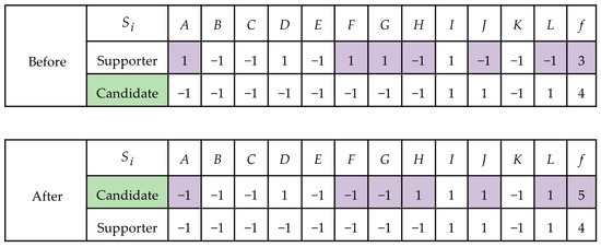
Figure 1.
Updating and replacing the supporting voter as the new candidate.
(b) Negative Advertisement
In this stage, widening the area of search space is required. The candidates try to attract voters from other parties. We presented Equation (28) to decide the number of voters, the candidate can attract from other parties (parties with highest fitness candidate):
where is the negative advertisement rate. After random selection, voters from other parties, the same steps, and equations that reflect the candidate’s influence on the supporters from outside will be used. The eligibility distance coefficient is given as follows:
where is the metric function of the eligibility of the candidate and voters. The formula of updating voters in parties is based on the following:
By using Equation (20), we can calculate the eligibility of the new supporters (potential solutions of ). Again, if there exists a voter with fitness value greater than the candidate, the candidate will be replaced by this voter.
(c) Coalition
In this stage, different parties cooperate and form a coalition to explore more areas in search space of . The coalition stage utilized the same steps and formulations as in negative advertisement. First, the two parties will be united randomly to decide who is going to be a new candidate after this union. First, find the eligibility distance function and distance coefficient by using Equation (29). After that, we decide the number of variables that needs to update in each voter from this combined party by using Equation (30). Now, all the voters’ fitness value has been updated. Finally, we compare the fitness value of the voters and old candidates. If the old candidate still has the highest fitness value, then the old candidate will proceed to election day. But if other situations happened, for instance, a voter has a higher fitness value compared to the old candidate. This fittest voter will be a new candidate to compete on election day with another party.
- 4.
- Stage 4: The Election Day
In this stage, the best solution (the candidate) in each party will be tested. If the solution has achieved the maximum fitness value , this solution will be announced as the optimal solution. Otherwise, the second iteration will take place. The steps will be repeated until the conditions are met. Figure 2 and Algorithm 1 summarize the steps involved in EA during the learning phase of HNN-RAN3SAT and Pseudo code of EA respectively.
| Algorithm 1: Pseudo Code of the Proposed HNN-RAN3SATEA | |
| 1 | Generate initial population |
| 2 | while or |
| 3 | Forming Initial Parties by using Equation (22) |
| 4 | fordo |
| 5 | Calculate the similarity between the voter and the candidate utilizing Equation (23) |
| 6 | end |
| 7 | {Positive Advertisement} |
| 8 | Evaluate the number of voters by using Equation (24) |
| 9 | fordo |
| 10 | Evaluate the reasonable effect from the candidate by using Equation (26) |
| 11 | Update the neuron state according to Equation (25) |
| 12 | if |
| 13 | Assign as a new |
| 14 | Else |
| 15 | Remain |
| 16 | End |
| 17 | {Negative advertisement} |
| 18 | Evaluate the number of voters |
| 19 | fordo |
| 20 | Evaluate the reasonable effect from the candidate by using Equation (29) |
| 21 | Update the neuron state according to Equation (30) |
| 22 | if |
| 23 | Assign as a new |
| 24 | Else |
| 25 | Remain |
| 26 | End |
| 27 | {Coalition} |
| 28 | fordo |
| 29 | Evaluate the reasonable effect from the candidate , by using Equation (29) |
| 30 | Update the neuron state according to Equation (30) |
| 31 | if |
| 32 | Assign as a new |
| 33 | Else |
| 34 | Remain |
| 35 | End |
| 36 | end while |
| 37 | return output the final neuron state |
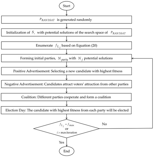
Figure 2.
Flowchart of the mechanism of EA for .
5. Exhaustive Search (ES)
Exhaustive search (ES) is one of the oldest techniques to enumerate and search for the solution. ES operates as a “generate and test” mechanism for all candidate solutions of the problem in search space until the optimal solution is obtained [37]. The main advantage of the ES algorithm is ES guarantees to obtain a solution (satisfied clause) by checking all candidate solutions in the search space. However, this algorithm consumes more computational time with intractable problems when the variables start increasing and the search space starts expanding exponentially with time [30]. Generally, ES algorithm consists of three main steps as stated below [38].
- 1.
- Step 1: Initialization.
Generate the potential bit strings .
- 2.
- Step 2: Fitness Evaluation.
Compute the number of satisfied clauses (fitness value of ) by using Equation (20).
- 3.
- Step 3: Test the solutions.
If the candidate has maximum fitness value, then the potential solution will return as output. Else, repeat the Step 1 and 2.
6. Summary of Learning and Retrieval Phase of HNN-RAN3SAT
This section demonstrates the full implementation of in HNN (or the HNN-RAN3SAT model). The main framework of the proposed HNN-RAN3SAT model is divided into two main phases. At first, the learning phase of the HNN-RAN3SAT model is introduced to check the satisfied assignment of by using learning algorithms to generate the optimal synaptic weights. In this study, Election Algorithm (EA) and Exhaustive Search (ES) are utilized as the learning algorithms. Then, the retrieval phase generates the correct final neuron states that lead to global minimum energy of the HNN-RAN3SAT model. The subsection below shows a detailed explanation of each phase in the HNN-RAN3SAT model.
6.1. Learning Phase in HNN-RAN3SAT
The purpose of embedding into the learning phase of HNN-RAN3SAT model is to create a network that will “behave” according to logical structure. has prominent characteristics such as bipolar representation and easy to represent in the form of neuron makes is compatible with HNN. The main concern in learning is the random structure of negated and positive literal in which leads to learning complexity of HNN to achieve . To reduce possible combinatorial explosion, EA is implemented in HNN to find the optimal assignment for that leads to . In this work, EA will utilize effective operator that has been mentioned in the previous section to computation burden for HNN-RAN3SAT. Conventionally, HNN will utilize ES [17] to obtain the optimal assignment that leads to . If the proposed EA failed to obtain to get the correct assignment, HNN-RAN3SAT will retrieve a suboptimal final state which leads to local minima energy. In other words, HNN-RAN3SAT will only retrieve the random pattern. In summary, the learning phase of HNN-RAN3SAT will require EA to find the assignment that leads optimal synaptic weight. From this synaptic weight, HNN will operate as a system that “behave” according to the proposed . The steps in executing learning phase of HNN-RAN3SAT model is summarized as follows:
- 1.
- Step 1: Convert into CNF type of Boolean Algebra.
- 2.
- Step 2: Assign neuron for each variable in .
- 3.
- Step 3: Initialize the synaptic weights and the neuron state of HNN-RAN3SAT.
- 4.
- Step 4: Define the inconsistency of the logic by taking the negation of .
- 5.
- Step 5: Derive the using Equation (6) that is associated with the defined inconsistencies in Step 4.
- 6.
- Step 6: Obtain the neuron assignments that leads to (using EA and ES), .
- 7.
- Step 7: Map the neuron assignment associated with the optimal synaptic weight. Precalculated synaptic weight can be obtained by comparing with the Final Energy function in Equation (15).
- 8.
- Step 8: Store synaptic weights as a Control Addressable Memory (CAM).
- 9.
- Step 9: Calculate the value of by using Equation (17).
6.2. Retrieval Phase in HNN-RAN3SAT
After completing the learning phase of HNN-RAN3SAT, we will be using the synaptic weight obtained in the learning phase into the retrieval phase. This is a phase where the HNN demonstrate the behavior of . According to [39], the neuron state produced by HNN should have non-linear relationship with the input state. Inspired by this motivation, we utilize Hyperbolic Tangent Activation Function (HTAF) [40] to squash the neuron output. The quality of the final neuron state will be checked based the differences between the calculated energy function and minimum energy function . The following steps explain the calculation involved in retrieval phase of HNN-RAN3SAT model.
- 1.
- Step 1: Calculate the local field of each neuron in HNN-RAN3SAT model using Equation (8).
- 2.
- Step 2: Compute the neurons state value by using HTAF [40] and classify the final neuron state based on Equation (9).
- 3.
- Step 3: Calculate the final energy of the HNN-RAN3SAT model using Equation (15).
- 4.
- Step 4: Verify whether the final energy obtained satisfy the condition in Equation (18). If the difference in energy is within the tolerance value, we consider the final neuron state as global minimum solution.
Worth mentioning that, the effective learning phase of HNN-RAN3SAT will optimize the state produced by the retrieval phase. In this case, the choice of Metaheuristics Algorithm in obtaining is paramount in ensuring the optimality of HNN-RAN3SAT.
7. Experimental Setup
The experimental setup for this study mostly follows the experiment set of [27]. The simulations for HNN-RAN3SATEA were executed on Dev C++ (Developed and Manufactured by Embarcadero Technologies, Inc, Texas, US) Version 5.11 running on the computer that has 4GB RAM and using Windows 8. The CPU threshold time for generating data will be 24 h and the simulation will be terminated if CPU time exceeds 24 h [41]. Notably, the models used a simulated dataset obtained by Dev C++ with 100,000 number of learning to generate . Here, the probability of generating a literal is equal to the probability of generating a negated literal. Additionally, the logical structure of consists of first, second and third order logic. The selection of clauses in a logical structure is set by random. Besides that, the use of HTAF is important in this study since we want to generate correct final neuron states. The characteristics of HTAF that were differentiable and nonlinear is important in constructing the proposed model as HTAF is a mathematical function that attached to the neurons. The nonlinear HTAF helps the proposed model to learn complex patterns in data. Additionally, the proposed model still operates if no activation function is utilized. However, the proposed model unable to learn the pattern of classification problem which is the same as a linear classifier. The effectiveness of this paper will be tested by comparing two models: HNN-RAN3SATEA and HNN-RAN3SATES in terms of accuracy and efficiency. The parameter assignments in HNN-RAN3SATEA and HNN-RAN3SATES models are summarized in Table 1 and Table 2.

Table 1.
List of parameters utilized in HNN-RAN3SATEA model.
Table 2.
List of parameters utilized in HNN-RAN3SATES model.
8. Performance Metric for HNN-RAN3SAT Models
Four types of matrices performance will be utilized to evaluate the efficiency of HNN-RAN3SAT models in terms of error analysis, energy analysis and similarity index. For error analysis, the evaluation for the learning and retrieval phase will be based on root mean square error (RMSE), mean absolute error (MAE), mean absolute percentage error (MAPE). Meanwhile, global minima ratio is evaluated in energy analysis. Finally, Jaccard (J), Sokal Sneath (SS), Dice (D), and Kulczynski (K) are evaluated in similarity index. The purposes of evaluating each metric will be explained further below.
8.1. Root Mean Square Error (RMSE), Mean Absolute Error (MAE), and Mean Absolute Percentage Error (MAPE)
Root mean square error (RMSE) and mean absolute error (MAE) has been widely used in evaluating the accuracy of the models by measuring the difference between the values predicted by the model and the target values. RMSE is sensitive to outliers, and it is more appropriate to use than the MAE when the model follows the normal distribution [42]. Note that, mean absolute percentage error (MAPE) is the average of absolute percentage errors. MAPE is highly adapted for predicting applications, especially in situations sufficient data is available [43]. In real-world applications, MAPE is frequently used when the amount to predict does not equal zero. This is due to the MAPE produces infinite values when the actual values are zero or close to zero, which is a common occurrence in some fields [44]. In the current study, the formula of calculating RMSE, MAE, and MAPE in the learning phase is modified as [27]:
where is the highest fitness achieved in the network based on the HNN-RAN3SAT model, is the fitness values that achieved during learning phase and is the number of iterations before . Notably, is the iterations generated by the simulation before achieved its full iteration, or can be written as . The RMSE, MAE, and MAPE in the testing phase will be expressed as [43]:
where is the target value (global energy) and refers to the predicted value (calculated energy) by the proposed model.
8.2. Global Minima Ratio
is the ratio between the total global minimum energy and the total number of runs in the testing phase [22]. can be expressed as:
where is the number of trials, is the number of neuron combination and is the number of global minimum energy of the proposed model. This measurement is good to compare the performance of the models since HNN-RAN3SATES when the number of variables increases the model fails to reach global minimum energy.
8.3. Similarity Index
A similarity index measures the relationship between final states of the neuron in the retrieval phase and benchmark neurons (the ideal neuron state) that can be defined as [18]:
Here, some similarity indices for neuron state that will be utilized in this study to distinguish global minimum solutions produced by HNN presented in Table 3 and Table 4.
Table 3.
Similarity indices used in the current study.
Table 4.
Neuron state for parameters in similarity index.
The neuron variation of HNN model is the number of solutions can be produced in each neuron combination and can be calculated by Equations (39) and (40):
where is the total number of solutions produced by the HNN model. is the solution produced in the i-th trial.
9. Result and Discussion
Firstly, to test the performance of the proposed HNN-RAN3SAT model, the comparison between the learning algorithms of EA and ES is analyzed in each phase. Various evaluation metrics utilized to study the influence of different learning algorithms in the HNN-RAN3SAT model. All compared learning algorithms are conducted independently on the simulated datasets generated randomly by Dev C++. Further analysis on the performance of HNN-RAN3SATEA and HNN-RAN3SATES revolves around the learning phase and retrieval phase performance analysis.
9.1. Learning Phase Performance
This section evaluates the capability of the proposed EA in doing in HNN (HNN-RAN3SATEA). The proposed model will be compared with the benchmark learning method proposed by [28] (HNN-RAN3SATES). The main emphasis of this comparison is to evaluate whether the proposed learning method can embed the behavior of into HNN model. Inspired by works such as [45,46], this section will utilize learning error metrics such as Root Mean Square Error , Mean Absolute error and Mean Absolute Percentage Error .
Figure 3, Figure 4 and Figure 5 demonstrate the , and results for HNN-RAN3SATES and HNN-RAN3SATEA respectively for until neurons. The graphs emphasize the accuracy of the learning phase of the proposed model as opposed to the conventional model, where lower error evaluations indicating higher accuracy. Generally, similar trends observed in Figure 3, Figure 4 and Figure 5, where HNN-RAN3SATES recorded the highest measures as compared to HNN-RAN3SATEA for every NN. Based on the results, HNN-RAN3SATEA outperformed HNN-RAN3SATES when the number of neurons increased. According to Figure 3, the deviation of the error is much lower as the number of neurons increased. Note that the high value of manifests the significant gap between the average fitness difference of the HNN-RAN3SAT model with the lowest fitness value. Despite acquiring single objective function during learning phase, EA managed to complete the learning phase with lower value of compared to the conventional method. Note that consists of where and that requires effective state update. By increasing in will create a fitness gap between optimal string fitness and the current fitness. In terms of probability of obtaining , is observed to achieve satisfied clause or but will result in more entry for synaptic weight structure. To make matters worse, probability for reduced exponentially as the number of . In this case, the high value is due to high number of in . Next, to effectively update all the state combination in , HNN-RAN3SATEA employed positive advertisement which accelerates the learning to achieve . The potential neuron space was divided into several parties where the eligibility distance coefficient increases both fitness of the most eligible candidate (highest fitness) and the least eligible candidate (lowest fitness). If the fitness gap is high (between the candidate and the voter), the next positive advertisement campaign will further reduce the gap until the best candidate is found. Another interesting observation is the most eligible candidate that achieve will assist other candidates in the party via update of . A similar mechanism was employed in other parties that potentially reduce the fitness gap between all solution in HNN-RAN3SATEA. However, the proposed positive advertisement in HNN-RAN-3SATEA has the capacity to reduce the eligibility of the voters or candidate but this effect is not obvious because there is no fluctuation for all values of . Unlike other metaheuristics algorithms that consist only 1 single space such as Genetic Algorithm, EA has additional parties with different updating rule. Hence, the fitness gap between the least eligible candidate with optimal fitness can be reduced which will result in lower value of . Based on Figure 3, value for HNN-RAN3SATEA remains low although the number of neurons increases to . This behavior has been reported in the work of [27] where EA effectively update the neurons state of lower order logical rule. Additionally, for HNN-RAN3SATES, the solution search space for this model is not well-defined and there is a high chance for the model to achieve non-improving solution or local maxima. This is due to very minimal effort by the model to improve the fitness of the current solution string. With the increase of number of neurons, HNN-RAN3SATES has irregular space that will increase the complexity of the method to . The increase of complexity will result in high value of . The high value of demonstrates low effectiveness of the proposed method in completing the learning phase of HNN.
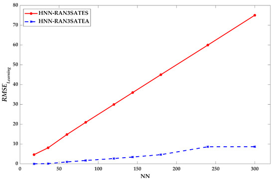
Figure 3.
for HNN-RAN3SAT model.
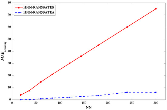
Figure 4.
for HNN-RAN3SAT model.
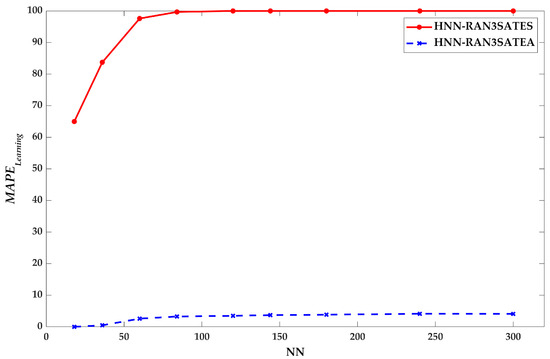
Figure 5.
for HNN-RAN3SAT model.
On the other hand, according to Figure 4, the absolute error for HNN-RAN3SATEA is much lower as the number of neurons increased. Note that, the high value of signifies the actual difference between the average fitness and the maximum fitness of the HNN-RAN3SAT model. The key strategy by HNN-RAN3SATEA to maintain a low value is the negative advertisement. Negative advertisement capitalizes the exploration capability to identify the potential optimal candidates. During negative advertisement, the composition of the voters in HNN-RAN3SATEA changed where eligible candidates have been attracted to the stronger party. The change of position of the voter will increase the chances for the voter to increase eligibility because the stronger party has a higher eligibility value. Thus, individual eligibility for all the voters and candidates will increase and the absolute error reduced dramatically. Indirectly, negative advertisement divides the composition of the strong party that has less of compared to weak party that has more of . Although there is potential and during the change of position but the value suggested most of the error accumulated from the that is very sensitive to the state change. This finding has a good agreement with the work of [27,28] where is the main Satisfiability issue in Random Satisfiability. Note that, third order clause in was reported to be easily satisfied due to more state option, thus showing the potential value for is almost zero. It is worth mentioning that negative advertisement will improve the candidate of the party because the new positioning of the voters into a new party will change the solution space of the party. For example, if one of the voters that has was attracted to other party in which the candidate of the party has , the change of candidate will occur. The new positioning of the candidate will improve the overall eligibility of the party. Another scenario to consider is when all the candidates from the weak party move to strong party and the overall eligibility of the candidate in the weak party decreases, thus increasing the value. In this case, the weak party will be slowly disregarded during the next trial of HNN-RAN3SATEA. As of state update, negative advertisement allows a similar update to positive advertisement. The update will increase the individual fitness in all parties and hence, reduce the value of . Additionally, HNN-RAN3SATES does not acquire any systematic exploration method. The fitness value for each individual solution string varies from near-optimal fitness to very low fitness without any potential improvement. There is a high chance that both and will not satisfied during the next iteration. The inefficient state exploration will result in high value. In short, the result in Figure 4 confirms that HNN-RAN3SATEA offers great optimization capability to diversify the candidates and provide more chances for the individual voter to improve with respect to the current candidate. The value demonstrates the compatibility of the as a logical rule in HNN as the number of neuron increase.
As shown in Figure 5, the percentage error for HNN-RAN3SATEA is lower compared to HNN-RAN3SATES as the number of neurons increased. One of the key hindrances of learning in HNN is the random assignment of the negated literal. Negated literal in mostly impact first and second order logic where the probability to obtain is high. Note that, the high value of signifies a high percentage of unsatisfied clause of . HNN-RAN3SATEA managed obtain lower value of compared to HNN-RAN3SATEA because the effectiveness of Coalition to reduce the potential local maxima during the learning phase. According to Figure 5, the value when is almost zero compared to HNN-RAN3SATES that reaches 60–70% percentage of unsatisfied clauses. This implies the effectiveness of the HNN-RAN3SATEA in discovering other solution space if the HNN achieves the non-improving solution. During Coalition, eligibility of the candidate in the strong parties improved by combining the effect of distance coefficient from another strong party. In this case, the eligibility of the candidate will increase with respect to other eligible candidates from other parties. In other words, Coalition expedites the process of finding neuron state that corresponds to during learning phase. In summary, HNN-RAN3SATEA managed to complete the learning phase for all values of compared to HNN-RAN3SATES that achieve 100% percentage error when .
9.2. Retrieval Phase Performance
This section encompasses the analysis of the retrieval phase for the proposed model, HNN-RAN3SATEA with the benchmark model, HNN-RAN3SATES as proposed by [28] in terms of error evaluation, energy analysis, neuron variation and similarity analysis measure. The testing error evaluations are based on the RMSE, MAE and MAPE to comply with learning error evaluation. The energy evaluation will utilize the ratio of global solution as coined by the work of [18]. In terms of similarity index (SI), several performance metrics such as Jaccard (), Sokal Sneath (), Dice () and Kulczynski Index () inspired by the work of [28] will be implemented in this study. Building from the similarity aspects, the total variation also will be considered to assess the quality of the final neuron state. As of physical meaning for each figure, Figure 6, Figure 7 and Figure 8 demonstrate the accuracy of the testing phase (retrieval phase) of our proposed model with respect to the benchmark model. Lower error measures the effectiveness of the HNN-RAN3SAT model to generate the final state that achieved global minimum energy. The numerical comparison of the number of global minimum energy in the form of ratio is shown in Figure 9. Figure 10, Figure 11, Figure 12 and Figure 13 demonstrate the similarity indices of the final states obtained by the HNN-RAN3SAT model. The higher index depicts more overfitting behavior of the final state produced by HNN-RAN3SAT model. As of Figure 14, the value in the graph indicates the effectiveness of the HNN-RAN3SAT model in retrieving different final state from each other. In other words, high value of indicates HNN-RAN3SAT model produce non-repeating final neuron state which leads to more diversified neuron states.
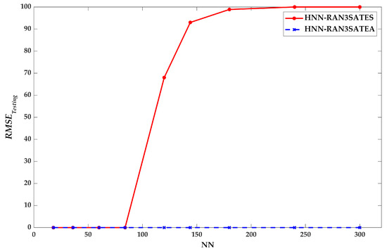
Figure 6.
for HNN-RAN3SAT model.
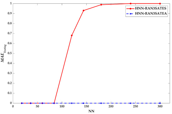
Figure 7.
for HNN-RAN3SAT model.
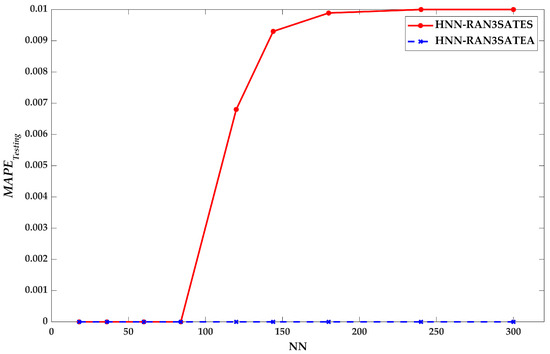
Figure 8.
for HNN-RAN3SAT model.
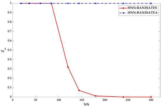
Figure 9.
for HNN-RAN3SAT model.
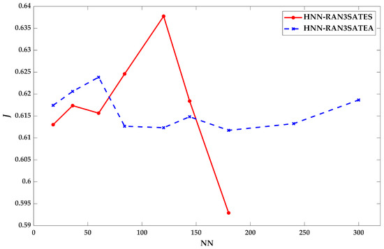
Figure 10.
(Jaccard) for HNN-RAN3SAT model.
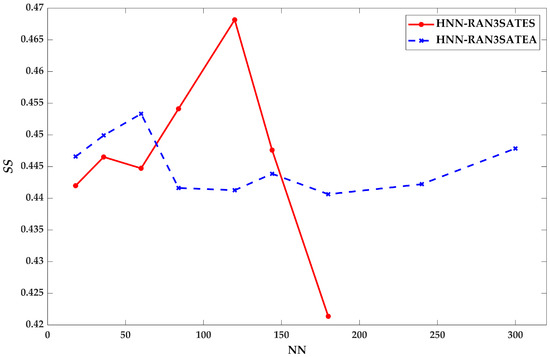
Figure 11.
(Sokal Sneath) for HNN-RAN3SAT model.
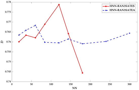
Figure 12.
(Dice) for HNN-RAN3SAT model.
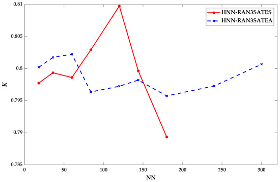
Figure 13.
(Kulczynski) for HNN-RAN3SAT model.
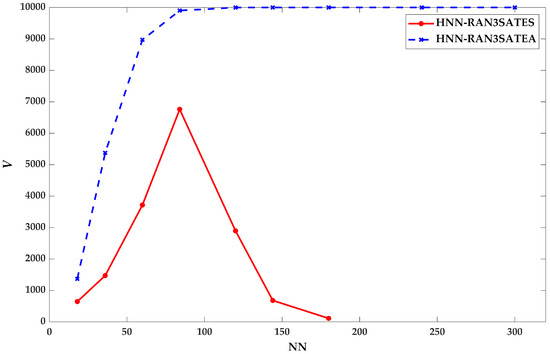
Figure 14.
(Neuron Variation) for HNN-RAN3SAT model.
According to Figure 6, Figure 7 and Figure 8, the error values that were reported for HNN-RAN3SATEA are , and for . This is due to the effective synaptic weight management that correspond to the “learned” during learning phase of HNN-RAN3SATEA. The capability of local search and global search operator in EA has successfully creates partitioning of the search spaces during learning phase, which improves the synaptic weight management during retrieval phase. However, the error measures for HNN-RAN3SATES model are growing rapidly, particularly when . The non-effective synaptic weight management in ES reduces the correctness of synaptic weights being retrieved during the retrieval phase. The outcomes will drive into the non-optimal states being retrieved and thus, HNN-RAN3SAT model starts retrieving the local minimum energy (refer Figure 9). Conversely, HNN-RAN3SATEA model consistently reaches the global minimum energy, and this is explained by the results in Figure 6, Figure 7 and Figure 8 which means HNN-RAN3SAT recalls the correct final states.
The results in Figure 9 demonstrate the performance of the HNN-RAN3SATEA with respect to HNN-RAN3SATES based on the ratio of global minimum solutions, . In addition, the consistent trend of HNN-RAN3SATEA which exhibit has verified the performance of HNN-RAN3SAT model in term of energy analysis. According to [28], the optimal synaptic weight management in EA contributes to the optimal testing phase in retrieving the consistent final neuron states. Therefore, the conditions such as the optimal final neuron states and correct synaptic weight, were the effect of the optimization operators in EA. Based on Figure 9, the fluctuations can be seen throughout the simulations for HNN-RAN3SATES except for , where the suboptimal states and non-systematic synaptic weight management have deteriorated the values. With this analysis, we can highlight the relationship between the ineffective learning by ES has influenced the learning phase, particularly when . The mechanism of ES, which deploys the intensive explorations within a larger search space, causing an ineffective learning phase that eventually affects synaptic weight management [46]. There will be a the possibility of retrieving non-optimal synaptic weight during the retrieval phase. Also, it needs to mention that in terms of solution space, EA approached the most systematic partition solution space in the model, which improves global and local search and finds the solution in all defined space. In contrast, ES has no effort of improving the global-local search in its solution space.
Furthermore, to investigate the quality of the solutions produced by HNN-RAN3SAT, similarity indices were calculated to compare each neuron of the string with the benchmark neuron that is determined by Equation (38) [28]. The general trend for Jaccard, Sokal Sneath, Dice and Kulczynski recorded by HNN-RAN3SATES as shown in Figure 10, Figure 11, Figure 12 and Figure 13 were increasing until the peak at , and stop getting any value when due to the presence of more local solutions. To support the analysis, the value of the global minima ratio that approaches zero within the aforementioned range. This indicates the variables of each state for (neurons of the string) obtained are not all equal the ideal neuron. HNN-RAN3SATEA model has similarity index values ranging from 0.4–0.8 and managed to generate the results for . The most interesting to ponder here is the difference in the similarity index values achieved in a specific number of neurons. For example, when , the similarity analysis were , , and . Lower similarity index was found to be recorded based on the and due to lower similarity values of the positive state as the positive benchmark states. This indicates the final states generated exhibits less overfitting, affecting the neuron variations. The effective synaptic weight management has been contributed due to the effectiveness of the local search and global search operators in EA as coined by [27]. The number of neuron variations as shown in Figure 14 also is very crucial to illustrate how HNN-RAN3SATEA can recall different solutions in each trial which means exploring different solutions and different areas in the search space. By taking a direct comparison towards when , where has manifested the lower similarity index reflects the higher variability of the final solutions. On contrary, the fluctuation in trend of can be seen in HNN-RAN3SATES where the model stops getting any value when . This is due to the non-effective synaptic weight management and training via ES, where the exploration being done in a tremendous search space, without any intervention of optimization operators [46].
Overall, HNN-RAN3SATEA outperformed the HNN-RAN3SATES in terms of the solution quality based on similarity analysis and the variability according to total variation measures. The final neuron states attained by the proposed model are certified to be less over-fit based on the lower similarity index and higher neuron variation achieved at the end of the simulations. In addition, the error evaluation and energy analysis also demonstrated the capability of HNN-RAN3SATEA in generating the global minimum solutions that correspond to the global minimum energy. The analysis also has verified the compatibility of with EA in HNN logic programming, with a promising potential to be applied in the logic mining [45] paradigm in the next exploration.
10. Conclusions
The main findings of this research prove the compatibility of logical representation analysis via Election Algorithm (EA) with HNN in both learning and retrieval phase based on error evaluations, energy analysis, similarity measures, and variability. The results via computer simulation have extensively shown that the formulated propositional logical rule consists of first, second, and third order logical rule has been successfully embedded optimally in Hopfield Neural Network, indicating the flexibility of the logical representation. Another finding of this research is that EA is an effective method for tackling as well as RAN2SAT in work [27]. In the context of learning algorithm, the results have manifested the capability of EA during the learning phase of logic in HNN as opposed to the conventional algorithm namely, Exhaustive Search (ES) by the learning accuracy and efficiency. In addition, particularly the proposed model has demonstrated the capacity in optimizing the retrieval phase based on the performance indicators such as error measures, energy analysis, similarity index, and variability evaluation. Based on the analysis, all research objectives have been achieved after conducting the simulations.
The research raises important questions about the role of EA that has verified the capability of the higher-order propositional logic in HNN, specifically referring to the proposed non-systematic RAN3SAT logic. Based on the promising results obtained by encoding in HNN with EA, the new logical structure RAN3SAT can be further applied in logic mining due to its flexibility to represent non-systematic data. Additionally, the proposed logical structure can be extended as a main logic mining representation of various data ranging from medical, engineering, and finance data set. The potential performance metrics such as median absolute deviation (MAD) [47], area under curve (AUC) [48], F1 score [49], logarithmic loss [50], and dissimilarity index analysis can be potentially considered in future work to enhance the analysis.
Author Contributions
Conceptualization, methodology, writing—original draft preparation, M.M.B.; validation, S.Z.M.J.; formal analysis, N.E.Z.; investigation, resources, funding acquisition, M.S.M.K.; writing—review and editing, M.A.M.; visualization, A.A.; project administration, S.A.K. All authors have read and agreed to the published version of the manuscript.
Funding
This research was funded by Fundamental Research Scheme Grant (FRGS), grant number 203/PMATHS/6711804.
Acknowledgments
The authors would like to express special dedication to all of the researchers from AI Research Development Group (AIRDG) for the continuous support.
Conflicts of Interest
The authors declare no conflict of interest.
References
- Hopfield, J.J.; Tank, D.W. “Neural” computation of decisions in optimization problems. Biol. Cyber. 1985, 52, 141–152. [Google Scholar]
- Hemanth, D.J.; Anitha, J.; Mittal, M. Diabetic retinopathy diagnosis from retinal images using modified Hopfield neural network. J. Med. Syst. 2018, 42, 1–6. [Google Scholar] [CrossRef]
- Channa, A.; Ifrim, R.C.; Popescu, D.; Popescu, N. A-WEAR Bracelet for detection of hand tremor and bradykinesia in parkinson’s patients. Sensors 2021, 21, 981. [Google Scholar] [CrossRef]
- Channa, A.; Popescu, N.; Ciobanu, V. Wearable solutions for patients with parkinson’s disease and neurocognitive disorder: A systematic review. Sensors 2020, 20, 2713. [Google Scholar] [CrossRef]
- Veerasamy, V.; Wahab, N.I.A.; Ramachandran, R.; Madasamy, B.; Mansoor, M.; Othman, M.L.; Hizam, H. A novel rk4-Hopfield neural network for power flow analysis of power system. Appl. Soft Comput. 2020, 93, 106346. [Google Scholar] [CrossRef]
- Chen, H.; Lian, Q. Poverty/investment slow distribution effect analysis based on Hopfield neural network. Future Gener. Comput. Syst. 2021, 122, 63–68. [Google Scholar] [CrossRef]
- Cook, S.A. The Complexity of Theorem-Proving Procedures. In Proceedings of the Third Annual ACM Symposium on Theory of Computing, New York, NY, USA, 3 May 1971; Association for Computing Machinery: New York, NY, USA, 1971; pp. 151–158. [Google Scholar]
- Fu, H.; Xu, Y.; Wu, G.; Liu, J.; Chen, S.; He, X. Emphasis on the flipping variable: Towards effective local search for hard random satisfiability. Inf. Sci. 2021, 566, 118–139. [Google Scholar] [CrossRef]
- Lagerkvist, V.; Roy, B. Complexity of inverse constraint problems and a dichotomy for the inverse satisfiability problem. J. Comput. Syst. Sci. 2021, 117, 23–39. [Google Scholar] [CrossRef]
- Luo, J.; Hu, M.; Qin, K. Three-way decision with incomplete information based on similarity and satisfiability. Int. J. Approx. Reason. 2020, 120, 151–183. [Google Scholar] [CrossRef]
- Hitzler, P.; Hölldobler, S.; Seda, A.K. Logic programs and connectionist networks. J. Appl. Log. 2004, 2, 245–272. [Google Scholar] [CrossRef] [Green Version]
- Abdullah, W.A.T.W. Logic programming on a neural network. Int. J. Intell. Syst. 1992, 7, 513–519. [Google Scholar] [CrossRef]
- Pinkas, G. Symmetric neural networks and propositional logic satisfiability. Neural Comput. 1991, 3, 282–291. [Google Scholar] [CrossRef] [PubMed]
- Abdullah, W.A.T.W. Logic programming in neural networks. Malays. J. Comput. Sci. 1996, 9, 1–5. [Google Scholar] [CrossRef]
- Hamadneh, N.; Sathasivam, S.; Choon, O.H. Higher order logic programming in radial basis function neural network. Appl. Math. Sci. 2012, 6, 115–127. [Google Scholar]
- Mansor, M.A.; Jamaludin, S.Z.M.; Kasihmuddin, M.S.M.; Alzaeemi, S.A.; Basir, M.F.M.; Sathasivam, S. Systematic Boolean satisfiability programming in radial basis function neural network. Processes 2020, 8, 214. [Google Scholar] [CrossRef] [Green Version]
- Kasihmuddin, M.S.M.; Mansor, M.A.; Sathasivam, S. Discrete Hopfield neural network in restricted maximum k-satisfiability logic programming. Sains Malays. 2018, 47, 1327–1335. [Google Scholar] [CrossRef]
- Kasihmuddin, M.S.M.; Mansor, M.A.; Basir, M.F.M.; Sathasivam, S. Discrete mutation Hopfield neural network in propositional satisfiability. Mathematics 2019, 7, 1133. [Google Scholar] [CrossRef] [Green Version]
- Kasihmuddin, M.S.M.; Mansor, M.A.; Sathasivam, S. Hybrid genetic algorithm in the Hopfield network for logic satisfiability problem. Pertanika J. Sci. Technol. 2017, 25, 139–152. [Google Scholar]
- Mansor, M.A.; Kasihmuddin, M.S.M.; Sathasivam, S. Modified artificial immune system algorithm with Elliot Hopfield neural network for 3-satisfiability programming. J. Inform. Math. Sci. 2019, 11, 81–98. [Google Scholar]
- Sathasivam, S.; Mamat, M.; Kasihmuddin, M.S.M.; Mansor, M.A. Metaheuristics approach for maximum k satisfiability in restricted neural symbolic integration. Pertanika J. Sci. Technol. 2020, 28, 545–564. [Google Scholar]
- Zamri, N.E.; Alway, A.; Mansor, A.; Kasihmuddin, M.S.M.; Sathasivam, S. Modified imperialistic competitive algorithm in Hopfield neural network for boolean three satisfiability logic mining. Pertanika J. Sci. Technol. 2020, 28, 983–1008. [Google Scholar]
- Emami, H.; Derakhshan, F. Election algorithm: A new socio-politically inspired strategy. AI Commun. 2015, 28, 591–603. [Google Scholar] [CrossRef]
- Lv, W.; He, C.; Li, D.; Cheng, S.; Luo, S.; Zhang, X. Election campaign optimization algorithm. Procedia Comput. Sci. 2010, 1, 1377–1386. [Google Scholar] [CrossRef] [Green Version]
- Pourghanbar, M.; Kelarestaghi, M.; Eshghi, F. EVEBO: A New Election Inspired Optimization Algorithm. In Proceedings of the 2015 IEEE Congress on Evolutionary Computation (CEC), Sendai, Japan, 25–28 May 2015; IEEE: Piscataway, NJ, USA, 2015; pp. 916–924. [Google Scholar]
- Emami, H. Chaotic election algorithm. Comput. Inform. 2019, 38, 1444–1478. [Google Scholar] [CrossRef]
- Sathasivam, S.; Mansor, M.A.; Kasihmuddin, M.S.M.; Abubakar, H. Election algorithm for random k satisfiability in the Hopfield neural network. Processes 2020, 8, 568. [Google Scholar] [CrossRef]
- Karim, S.A.; Zamri, N.E.; Alway, A.; Kasihmuddin, M.S.M.; Ismail, A.I.M.; Mansor, M.A.; Hassan, N.F.A. Random satisfiability: A higher-order logical approach in discrete Hopfield Neural Network. IEEE Access 2021, 9, 50831–50845. [Google Scholar]
- Li, C.M.; Xiao, F.; Luo, M.; Manyà, F.; Lü, Z.; Li, Y. Clause vivification by unit propagation in CDCL SAT solvers. Artif. Intell. 2020, 279, 103197. [Google Scholar] [CrossRef] [Green Version]
- Kasihmuddin, M.S.M.; Sathasivam, S.; Mansor, M.A. Hybrid Genetic Algorithm in the Hopfield Network for Maximum 2-Satisfiability Problem. In Proceedings of the 24th National Symposium on Mathematical Sciences: Mathematical Sciences Exploration for the Universal Preservation, Kuala Terengganu, Malaysia, 27–29 September 2016; AIP Publishing: Melville, NY, USA, 2017; p. 050001. [Google Scholar]
- Sathasivam, S. Upgrading logic programming in Hopfield network. Sains Malays. 2010, 39, 115–118. [Google Scholar]
- Alway, A.; Zamri, N.E.; Kasihmuddin, M.S.M.; Mansor, A.; Sathasivam, S. Palm oil trend analysis via logic mining with discrete Hopfield Neural Network. Pertanika J. Sci. Technol. 2020, 28, 967–981. [Google Scholar]
- Jamaludin, S.Z.M.; Kasihmuddin, M.S.M.; Ismail, A.I.M.; Mansor, M.A.; Basir, M.F.M. Energy based logic mining analysis with Hopfield Neural Network for recruitment evaluation. Entropy 2021, 23, 40. [Google Scholar] [CrossRef]
- Abdullah, W.A.T.W. The logic of neural networks. Phys. Lett. A 1993, 176, 202–206. [Google Scholar] [CrossRef]
- Kumar, M.; Kulkarni, A.J. Socio-inspired optimization metaheuristics: A review. In Socio-Culture. Inspired Metaheuristics; Kulkarni, A.J., Singh, P.K., Satapathy, S.C., Kashan, A.H., Tai, K., Eds.; Springer: Singapore, 2019; Volume 828, pp. 241–266. [Google Scholar]
- Blum, C.; Roli, A. Hybrid metaheuristics: An introduction. In Hybrid Metaheuristics; Blum, C., Aguilera, M.J.B., Roli, A., Sampels, M., Eds.; Springer: Berlin/Heidelberg, Germany, 2008; Volume 114, pp. 1–30. [Google Scholar]
- Nievergelt, J. Exhaustive search, combinatorial optimization and enumeration: Exploring the potential of raw computing power. In International Conference on Current Trends in Theory and Practice of Computer Science; Springer: Heidelberg/Berlin, Germany, 2000; pp. 18–35. [Google Scholar]
- Mansor, M.A.; Kasihmuddin, M.S.M.; Sathasivam, S. Robust artificial immune system in the Hopfield network for maximum k-satisfiability. Int. J. Interact. Multimed. Artif. Intell. 2017, 4, 63–71. [Google Scholar] [CrossRef] [Green Version]
- Hopfield, J.J. Neural networks and physical systems with emergent collective computational abilities. Proc. Natl. Acad. Sci. USA 1982, 79, 2554–2558. [Google Scholar] [CrossRef] [Green Version]
- Mansor, M.A.; Sathasivam, S. Performance Analysis of Activation Function in Higher Order Logic Programming. In Proceedings of the 23rd Malaysian National Symposium of Mathematical Sciences (SKSM23), Johor Bahru, Malaysia, 24–26 November 2015; AIP Publishing: Melville, NY, USA, 2016; p. 030007. [Google Scholar]
- Kho, L.C.; Kasihmuddin, M.S.M.; Mansor, M.A. Logic mining in league of legends. Pertanika J. Sci. Technol. 2020, 28, 211–225. [Google Scholar]
- Chai, T.; Draxler, R.R. Root mean square error (RMSE) or mean absolute error (MAE)? Arguments against avoiding RMSE in the literature. Geosci. Model Dev. 2014, 7, 1247–1250. [Google Scholar] [CrossRef] [Green Version]
- Kim, S.; Kim, H. A new metric of absolute percentage error for intermittent demand forecasts. Int. J. Forecast. 2016, 32, 669–679. [Google Scholar] [CrossRef]
- Myttenaere, A.D.; Golden, B.; Le Grand, B.; Rossi, F. Mean absolute percentage error for regression models. Neurocomputing 2016, 192, 38–48. [Google Scholar] [CrossRef] [Green Version]
- Zamri, N.E.; Mansor, M.A.; Kasihmuddin, M.S.M.; Alway, A.; Jamaludin, S.Z.M.; Alzaeemi, S.A. Amazon employees resources access data extraction via clonal selection algorithm and logic mining approach. Entropy 2020, 22, 596. [Google Scholar] [CrossRef] [PubMed]
- Sathasivam, S.; Mansor, M.A.; Ismail, A.I.M.; Jamaludin, S.Z.M.; Kasihmuddin, M.S.M.; Mamat, M. Novel Random k Satisfiability for k≤ 2 in Hopfield Neural Network. Sains Malays. 2020, 49, 2847–2857. [Google Scholar] [CrossRef]
- Miah, A.S.M.; Rahim, M.A.; Shin, J. Motor-imagery classification using riemannian geometry with median absolute deviation. Electronics 2020, 9, 1584. [Google Scholar] [CrossRef]
- Liu, Y.P.; Li, Z.; Xu, C.; Li, J.; Liang, R. Referable diabetic retinopathy identification from eye fundus images with weighted path for convolutional neural network. Artif. Intel. Med. 2019, 99, 101694. [Google Scholar] [CrossRef] [PubMed]
- Sedik, A.; Iliyasu, A.M.; El-Rahiem, A.; Abdel Samea, M.E.; Abdel-Raheem, A.; Hammad, M.; Peng, J.; El-Samie, F.A.; El-Latif, A.A.A. Deploying machine and deep learning models for efficient data-augmented detection of COVID-19 infections. Viruses 2020, 12, 769. [Google Scholar] [CrossRef] [PubMed]
- Wells, J.R.; Aryal, S.; Ting, K.M. Simple supervised dissimilarity measure: Bolstering iForest-induced similarity with class information without learning. Knowl. Inform. Syst. 2020, 62, 3203–3216. [Google Scholar] [CrossRef]
Publisher’s Note: MDPI stays neutral with regard to jurisdictional claims in published maps and institutional affiliations. |
© 2021 by the authors. Licensee MDPI, Basel, Switzerland. This article is an open access article distributed under the terms and conditions of the Creative Commons Attribution (CC BY) license (https://creativecommons.org/licenses/by/4.0/).