1. Introduction
1.1. Hydrogen Economy
An envisioned future predicts a large use of hydrogen for vehicle or heat fuel, energy storage, and energy transport [
1]. The hydrogen economy would contribute to reducing green effect emissions and energy consumption. It stimulates economic growth and creates new jobs. However, the hydrogen economy also has to face technical challenges [
2], competition with other technologies and interrelates with technology strategies. A sustainable energy carrier for electric vehicles is one of the future uses of hydrogen. It is also a medium for utility-scale renewable energy storage and fuel distribution. Because hydrogen can be produced from fossil, nuclear or renewable sources, dependence on imports and improvement of energy security can be reduced by promoting hydrogen.
It has several significant advantages:
- −
A large amount of energy is generated by combustion;
- −
It is very abundant on Earth;
- −
Its combustion is carbon free;
- −
It is storable and can be an efficient means of storing electricity over long periods of time.
However, hydrogen carrier still faces several limitations:
- −
A large amount of energy is necessary for storage of hydrogen in compressed liquid or metal hydride form;
- −
Transport is less efficient than that of oil or gas due to this low density when comparing energy transported per unit of volume;
- −
Risks of detonation and flammability with air;
- −
Production process cost, particularly water electrolysis, remains high;
- −
For hydrogen cars, the establishment of a network of hydrogen stations requires considerable time and investment.
1.2. Hydrogen Car
The hydrogen car is considered as a “zero emission” vehicle [
2]. It is also called “fuel cell electric vehicle”, it runs on electricity like a conventional electric car. In hydrogen car, electricity is produced by a fuel cell (FC). This technic has several practical advantages.
Recharging takes less time than a full tank of gasoline, 3 to 5 min, compared to the few hours to recharge a battery-powered car.
The range is similar to that of a diesel vehicle: a full tank of hydrogen in a 700-bar pressurized tank can travel up to 400 km, two to three times more than battery-powered cars.
The FC is composed of several cells comprising two electrodes—an anode and a cathode—separated by a polymer membrane, which acts as an electrolyte. The electrochemical reactions between hydrogen injected at the anode and oxygen at the cathode lead to the production of electricity, heat and water. For this reason, FC is considered as a “clean” alternative to diesel and gasoline vehicles.
However, hydrogen car fuel cell suffers from the following disadvantages:
- −
The efficiency of the fuel cell is less than 50%;
- −
The efficiency of the energy chain is, on average, 25 to 30% efficiency for a hydrogen car and around 70% for an electric one;
- −
With high-pressure tanks, pipes, fuel cell, buffer battery, and electronic power, it is a more complex car; therefore, the reliability level is lower;
- −
Expensive fuel cell, incorporating problematic resource potential (platinum);
- −
Service station development is heavier and more expensive than electric charging stations;
- −
Hydrogen is a very dangerous gas which can induce strong explosions in the event of a problem or leak;
- −
The use of high pressure in tanks needs to be checked and controlled.
1.3. The Gas Mixture in End-Use Devices
The transport of hydrogen into the existing gas pipeline network has been proposed to increase the use of renewable energy systems [
3].
The injectable gas potential would be high enough to meet the demand. The injection of hydrogen in natural gas networks is called Power-to-Gas at a level less than 30%.
There is a large variation between EU countries on maximum blend level of hydrogen in natural gas grid in the range 0–12%, as seen in
Figure 1.
Adding hydrogen to natural gas links to the following problems:
- −
Material–hydrogen compatibility: the material of pipe networks can be tolerant of the presence of hydrogen;
- −
The density, viscosity, flammability limits, etc., are modified. This has an impact on maintenance and surveillance of gas networks;
- −
Modification of the control of the gas combustion parameters.
In France, the GRHYD project [
4],
Figure 2, applies the concept of Power-to-Gas used to transform surplus renewable electricity into hydrogen via the electrolysis of water and, thus, allow storage and recovery.
The mixture of hydrogen and natural gas, in varying proportions of hydrogen not exceeding 20% by volume, supply the boiler room in the new district to meet the demand of about 100 homes.
Gas systems will have to be redesigned to allow the delivery and recovery of this energy on a large scale. The construction of new infrastructures or the adaptation of existing networks and equipment to the properties of the hydrogen molecule will be slow developments, which will require significant investment. The injection of hydrogen into current gas networks is, thus, seen as a solution to reduce the costs associated with the construction of new infrastructure, while guaranteeing an outlet to produce carbon-free hydrogen [
5].
The addition of hydrogen in natural gas degrades over time the materials of transport and storage. This degradation depends on the ratio of hydrogen natural gas. After addition, several criteria need to be assessed:
- −
Hydrogen permeation through metals;
- −
Loss of pipe integrity;
- −
Adaptation of follow-up actions in service, surveillance, and maintenance of equipment.
In the following, the hydrogen embrittlement (HE) effect on design, maintenance and surveillance of smooth and damaged gas pipes is presented.
2. Hydrogen Embrittlement
It has been recognized since the end of the 19th century that hydrogen alters the steel mechanical properties [
6] by hydrogen embrittlement (HE). To unlight this phenomenon, tensile tests on API L X52 pipe steel have been performed and presented in
Figure 3. Specimens are loaded by an electrolytic process for HE and in air. One notes a reduction in failure elongation (38%) and a small reduction in yield stress and ultimate strength, respectively, 3.8% and 7.4%, as well as a reduction in fracture toughness. This phenomenon was first discovered by Johnson [
6]. There was also a reduction in fracture resistance.
Degradation of toughness increases the risk of gas line failure, loss of life, environmental damage, and economic loss associated with the repair of affected lines and loss of production.
Fracture initiation energy U
i exhibits a sudden drop for hydrogen concentration higher than a critical one when the material becomes brittle, as noticed by Capelle et al. [
7].
To understand the entry of hydrogen into metal, it is necessary to know the characteristics of the hydrogen evolution reaction and its distinct stages associated with the entire process. A double layer of hydrated atoms is transported on the surface. This hydrated form is separated in proton form and water and is adsorbed.
A discharge of the material is produced by electron donation. A combining hydrogen process occurs from atom to atom, atom to ion, or both. Finally, desorption and entry into the material results in the formation and diffusion of hydrogen.
Hydrogen moves easily between crystalline sites in steel; this is possible because it is small. It diffuses into metals by hetero-diffusion at infinite dilution. Trapping and accelerated transport atoms by mobile dislocations is the weakening mechanism. Dislocation rates are improved for perfect screw and wedge dislocations, partial dislocations, and grain boundary dislocations. The hydrogen atmosphere increases dislocation rate. This atmosphere protects interactions under elastic stress. This means that the separation distance between dislocations in a stack should collectively decrease.
The stack should approach the obstacle in the presence of hydrogen. A theoretical study has shown that hydrogen-induced softening and network expansion can cause shear localization in a material with a positive strain-hardening coefficient. Shear band bifurcation is a precursor to material failure. Hydrogen in metals accumulate in many locations. These locations are microstructures such as grain boundaries, inclusions, voids, dislocation tangles and dislocation networks, atoms in solute as well as in a solid solution. When hydrogen is fixed, failure will be controlled by the magnitude of the effects of hydrogen.
Hydrogen embrittlement is explained by several mechanisms, namely:
- −
Atomic bonds of metals weakening [
8];
- −
Enhancement of plasticity;
- −
Emission of dislocations/decohesion competition [
9];
- −
Molecular recombination in defects;
- −
Stress triaxiality.
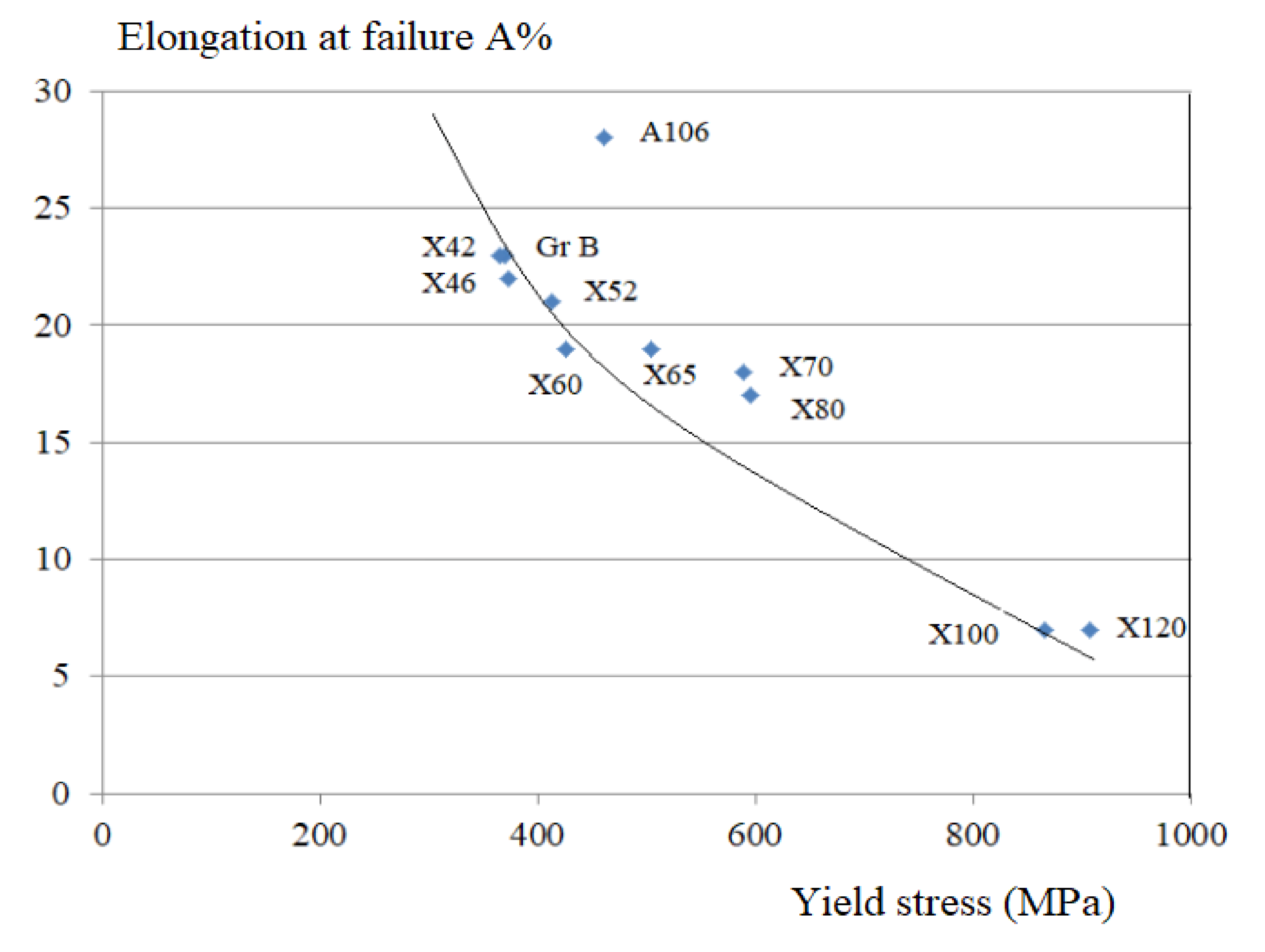
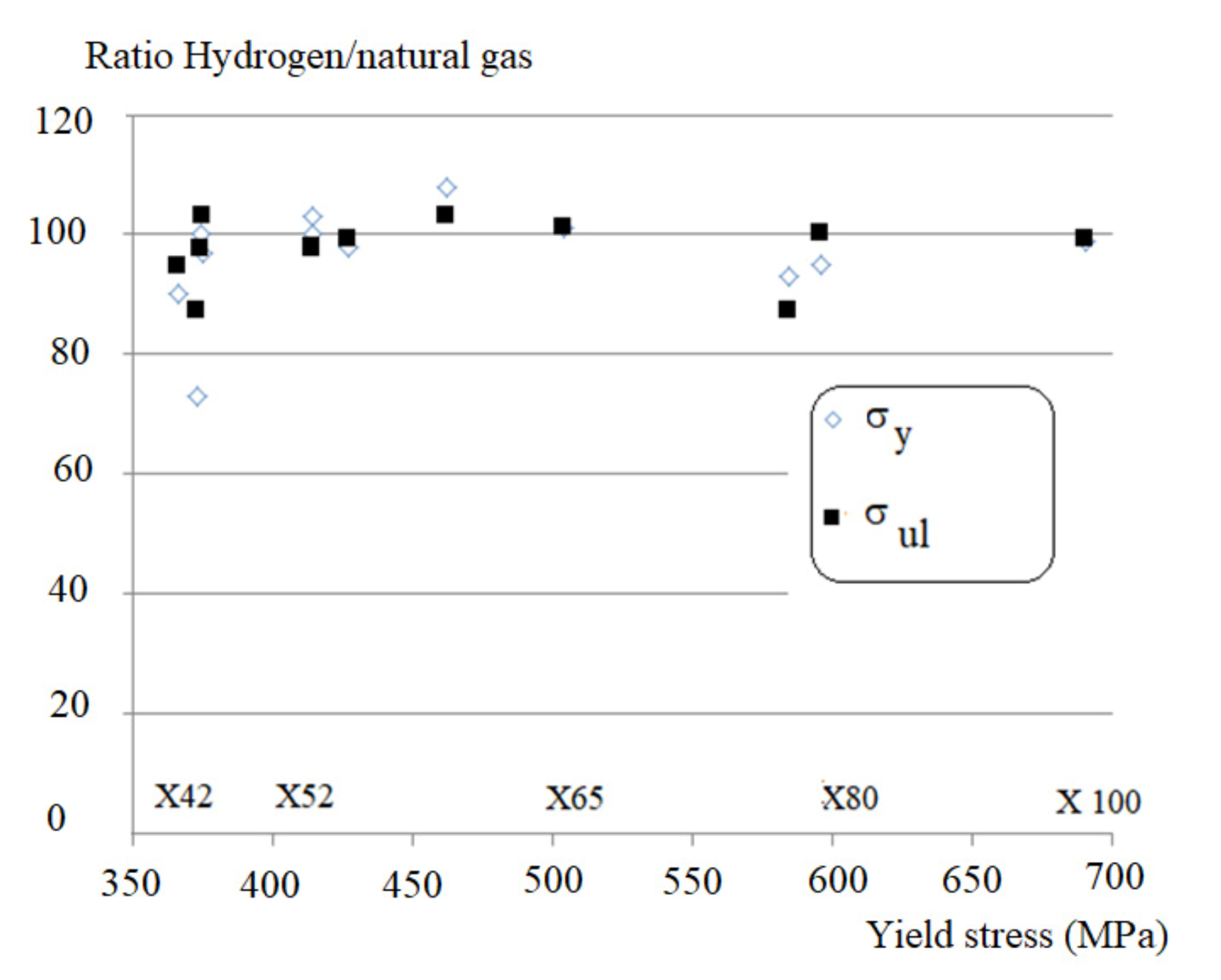
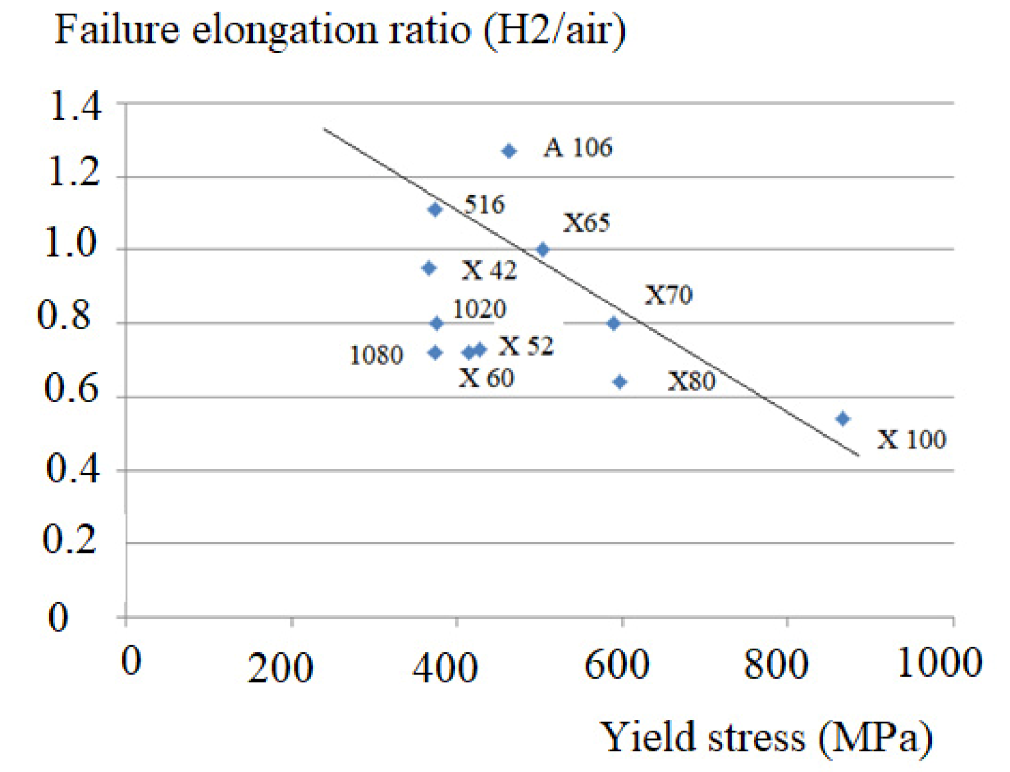
There is practically no effect of hydrogen embrittlement on yield stress and ultimate strength regardless of yield stress on pipe steels. The failure elongation ratio under influence of HE of several pipe steels versus yield stress is shown in
Figure 4. The ratio (A% (H
2)/A% (air)) decreases as the yield stress of the steel increases.
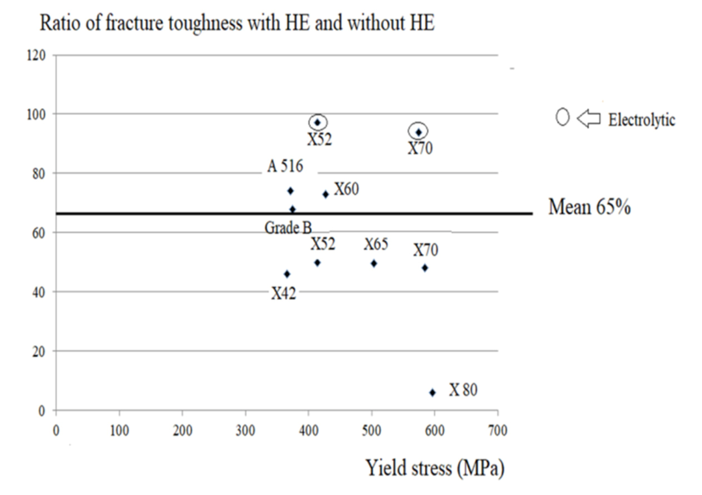
The fracture toughness is measured under conditions defined by standards. It is generally defined by the critical stress intensity factor KIc whose units are the MPa√m, the critical value of the energy parameter J defines at initiation (Jc) or, for a conventional value of stable crack propagation J0 whose units are KJ/m, the critical value of COD (critical crack opening displacement δc) whose units are millimeters.
By using the fracture toughness ratio under HE and without HE, one can avoid the influence of the toughness determination method K
IC, J
c or δ
c. Plotting versus yield strength shows a significant dispersion. Toughness decreases about 33% after HE,
Figure 5.
2.1. Fatigue Endurance
Fatigue endurance after hydrogen embrittlement has received less attention in the literature than fatigue crack propagation. It is important to note that high cycle fatigue life is made up of 70 to 90% of life duration. Long cracks propagating in the domain of Paris Law after hydrogen embrittlement are mainly concerned.
Wöhler curves were drawn by [
10] at both failure and initiation for API 5L X52 steel. The fatigue resistance at initiation curves is fitted by a power law:
is the fatigue initiation resistance,
Ni fatigue initiation numbers.
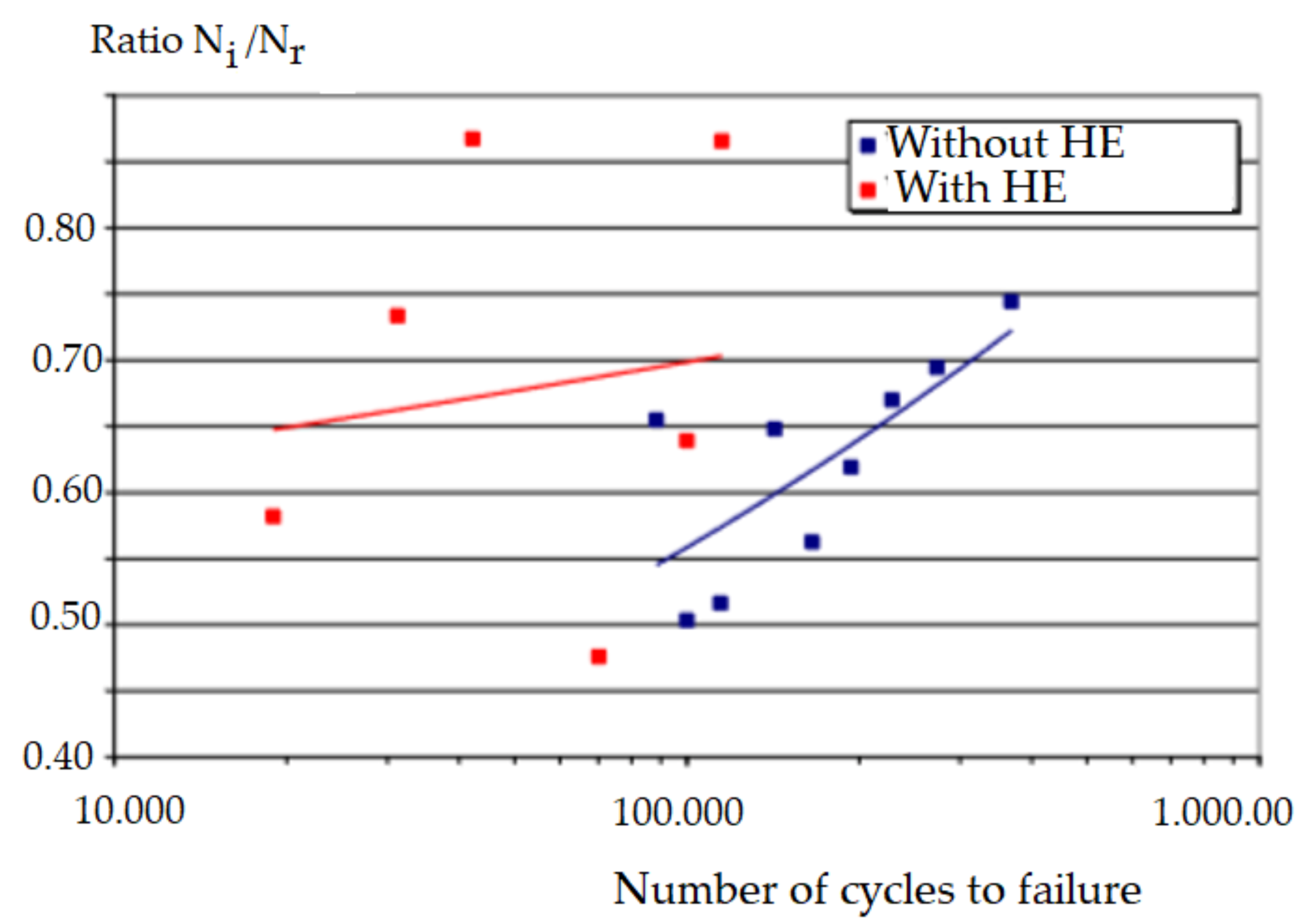
Figure 6 presents the
Ni/Nr ratio versus the number of cycles to failure
Nr. Values for API X52 pipe sttel are given in
Table 1.
Fatigue crack propagation is faster after HE and the Nr − Ni difference is reduced. Nr − Ni is precisely the number of propagation cycles. The Ni/Nr ratio suffers from a large scatter.
2.2. Fatigue Crack Propagation
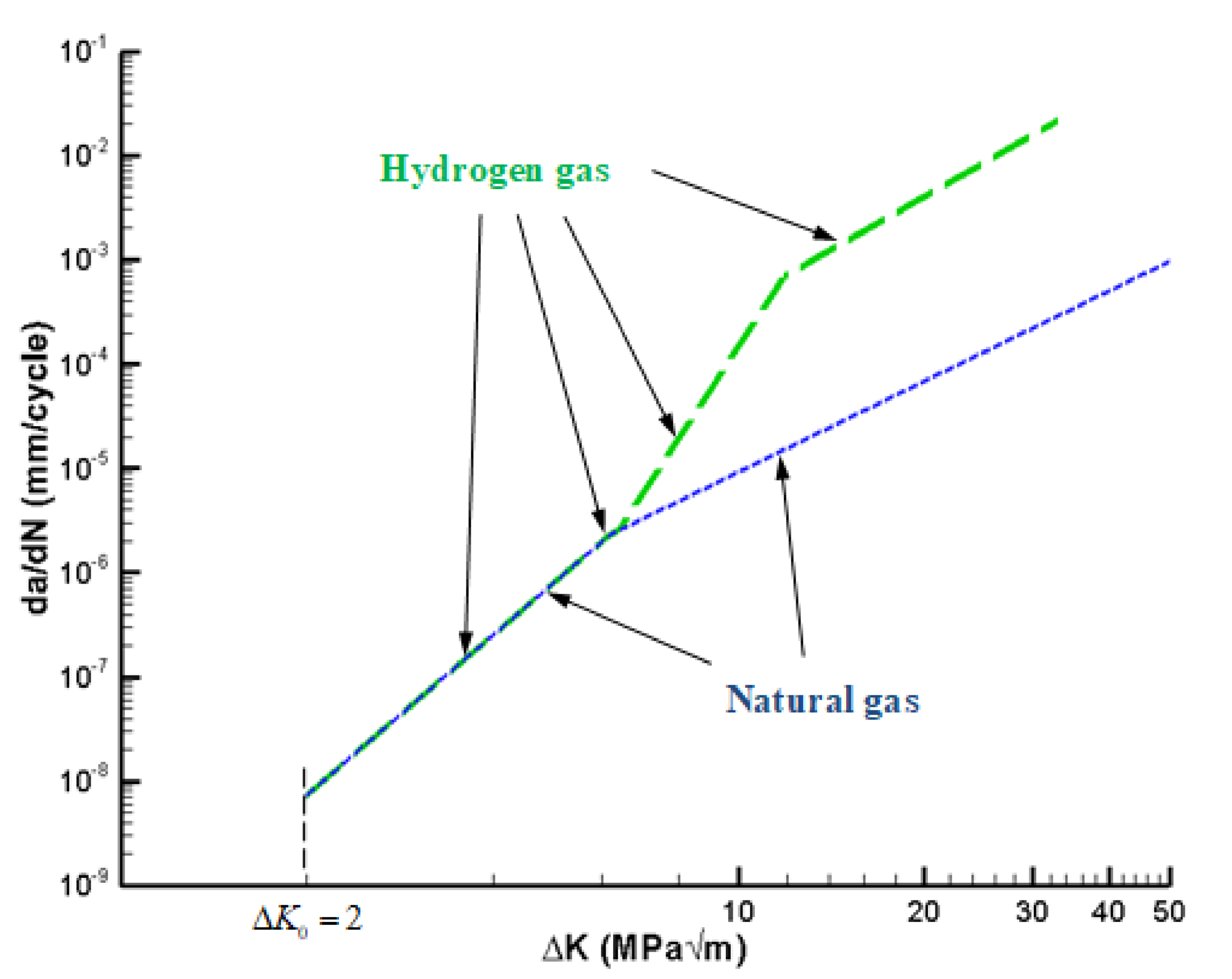
Hydrogen embrittlement affects fatigue crack propagation in stage II (Paris law regime) and particularly carbon pipe steels. Crack growth rate versus the maximum amplitude of the stress intensity factor in natural gas is presented in
Figure 7 by the solid line curve.
The process is made up of three stages:
- −
In the beginning, the growth rate increases along the sigmoidal curve governed by the fatigue crack threshold KTH, step 1. An increase in fatigue crack growth is attributed to hydrogen diffusion at the crack tip.
The growth rate is faster than the hydrogen diffusion rate with a low local concentration of hydrogen at the crack tip. At the start of step 2, the growth rate decreases. An equilibrium between the rate of growth of the crack and the rate of diffusion of hydrogen is achieved later. A plateau is obtained, and the crack growth rate remains constant. The equilibrium state is ensured by continuous hydrogen charging and crack growth.
Stage 3 begins when the crack growth resistance given by the toughness after HE K
IC,
H is less than intrinsic fracture toughness K
IC. The fatigue growth rate curve is governed only by K
TH and K
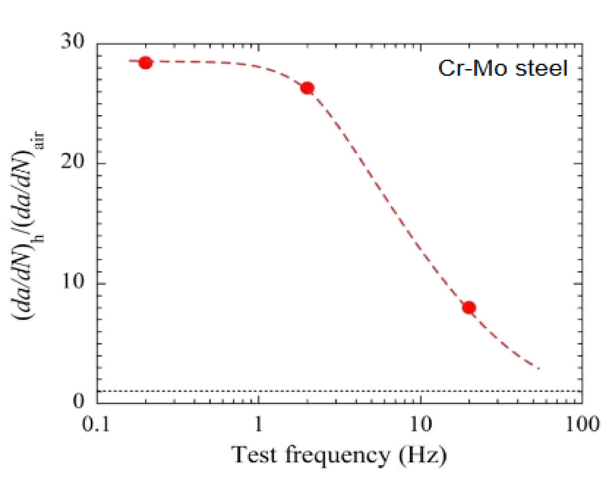
IC,H; both are drawn using dotted lines. The rate of fatigue crack growth is greatly increased—one to two orders of magnitude—by hydrogen embrittlement in the Paris law domain. Under hydrogen, the exponent of the Paris law increases strongly in the stress intensity factor range ΔK range [6–12 MPa√m]. Beyond that, it finds the same value as that of the law of growth of fatigue crack in air. According to [
12], the crack growth rate increases strongly for low frequencies and presents a plateau for a frequency lower than 1 Hz,
Figure 8.
3. Design against Brittle Fracture
Brittle fracture is taken into account in design by ensuring that the material must have a ductile behavior at service temperature. Therefore, ductility is sufficient to prevent cleavage triggering with a significant release of elastic energy. This concept concerns level I in several codes like API 579-1 ASME FFS-1 at [
13]. For that, the service temperature T
s is higher than the brittle-ductile transition temperature [DBTT) T
t. Codes or laws define the service temperature conventionally according to the country where the structure or component is constructed or installed.
In France, the service temperature is −20 °C. When this concept is based on fracture mechanics, designers ensure that the service temperature Ts is greater than fracture toughness transition temperature T0.
T
0 corresponds to a conventional fracture toughness value of K
Ic,ad = 100 MPa√m on the curve fracture toughness- temperature. More generally, reference temperature (RT), must be greater than service temperature:
ΔT is the uncertainty [
13].
The reference temperature is generally given by the designer or the codes to have a transition temperature close to those of the “structure or component”. Transition temperatures are specific to tests. The level of conservatism in the design depends on this choice. Transition temperature is sensitive to constrain according to [
14]. It decreases when they constrain due to thickness, triaxiality or loading mode decreases. A test providing a constrain value close to that of the structure minimizes the conservatism. It should be noted that the choice of Charpy test piece is highly conservative due to the high constrain specimen because the bending test with high triaxiality induces via sharp V notch.
For thin pipes, standard, Charpy test specimens of 10 mm thickness cannot be extracted. In this case, mini Charpy test are preferred. Experimental results are fitted according to a hyperbolic tangent law (Oldfield) [
15].
Constants A
CV, B
CV, C
CV are related to energy level of the ductile plateau USE, energy level at brittle plateau LES, DBTT is the ductile-brittle transition temperature.
For pipe steel API 5 L X60, the mini-Charpy energy–temperature curve is presented in
Figure 9. Data are fitted according to Equation (3). A
CV, B
CV, C
CV and, D
cv are reported in
Table 2.
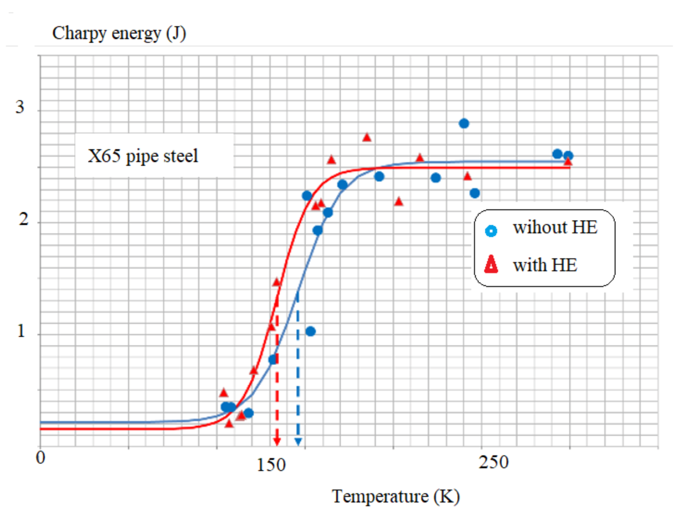
The Charpy energy–temperature curve exhibits a slightly different behavior from that obtained with the material without HE. The brittle and ductile plateau levels are similar, but the transition temperature define by D
CV is increased from 10 °C, i.e., very few. The authors of [
16], performing tests on Standard Charpy specimens, also made of X65 pipe steel, noted no shift in transition temperature defined at the energy level of 27 joules.
4. Design Factor for Smooth Pipe Transporting Hydrogen Blended with Natural Gas
When the service pressure p
s exceeds the Maximum Admissible Operating Pressure (MAOP), the leak is considered to happen on smooth pipes.
The calculation formula of ASME code [
1] involves partial safety coefficients. Reduction in thickness has to be considered.
e: nominal thickness;
f0: design factor;
D: nominal outside diameter;
E: Weld factor;
Hf: Material performance factor;
S: specified minimum yield strength;
T: Temperature derating factor.
The specified minimum yield strength S is given from pipe steel designation, for example, API 5L X (
) as
The maximum admissible stress
σad is given by the following formula:
where σ
y, ref is the material reference yield stress and f
0 is the design factor.
Values of design factor for the natural gas grid are given by code [
17] in France. Value depends on pipe localization as can be seen in
Table 3.
The yield stress of pipes steel is not affected by hydrogen embrittlement—see
Figure 10. However, this only consideration leads to the same design factor being kept for the same admissible stress for hydrogen embrittlement. However, hydrogen transport needs to also consider the risk of explosion due to the large inflammability range and low ignition energy. For transport of hydrogen in pipes, other design factors f
0 have been chosen by American code ASME B31.12-2004 [
18] with respect to pipeline location, as indicated in
Table 4.
Four cases have been defined for code division 2 (high constraint environment)
Class 1 (corresponds to an environment with high constraint);
Class 2 (corresponds to a rural environment);
Class 3 (corresponds to a peri-urban environment);
Class 4 (corresponds to a highly urbanized environment).
According to the pipe steel and service pressure, the design factor is used for the determination of pipe diameter.
Based on expert judgments, the design factor is a deterministic factor. New trends are based on a probabilistic approach. The following general equation is use for calculated the risk associated with pipeline transport:
Risk = Frequency of pipeline failure × Probability of ignition × Human, economic or societal consequences.
Codes consider an individual and human risk, i.e., the probability for a given pipeline length, that a person will become a victim in a year. Global risk is the product of all failures and consequences (per year). The risk is given by the probability that a point located near a pipe and at a known distance could be exposed to an effect of an intensity greater than a reference level. This probability is expressed by:
where:
Pr (F) leak probability after failure;
Pr (Q) probability of flow greater than a critical value;
Pr (I) probability of ignition;
Pr (EF) probability of lethal effects greater than a threshold value;
Pr (pers) probability of the presence of a person;
L length of the pipeline;
Cev coefficient to consider the environment of the pipeline;
Crr risk reduction factor considering risk reduction measures.
If
Pr (Risk) is distributed according to a simple Weibull law. The safety factor is defined as:
where m is the Weibull exponent.
Table 5 presents a comparison between probabilistic design factor f
0,
prob (present method) [
18] and deterministic one f
0,
det [
17]. Deterministic values differ between the three locations and are more conservative. In [
17], no description of arguments that leads to values of deterministic design factor is presented.
This is valid only for pipe geometry and steel API 5L X60. A larger study on other pipe geometry and steels could not strongly modify the conclusion.
The coefficient of variation (COV) of the steel yield stress is incorporated in Equation (9). Therefore, the design factor is sensitive to the COV of material properties.
Figure 11 presents the influence of yield stress COV on MAOP. This figure indicates that, for an urban area, the MAOP decreases by 90% and the design factor by 85% when COV vary in the range [0.05–0.20].
If we assume that that the economical threshold for MAOP, called MAOP* is 50 MPa, one cannot tolerate in the pipe networks, some part with vintage steels exhibiting a COV greater than 0.15, see
Figure 11.
5. Maintenance of Cracked Pipe
Very long pipes are made by in situ welding. Defects such as porosities, slag inclusions, melts or cracks are often present in the weld or the heat-affected zone (HAZ). Cracks have an irregular shape and are considered the most severe defects. For conservative reasons, they are considered elliptical or semi-elliptical surface cracks. By enclosing the irregular crack in a rectangle of length 2c and width 2a for internal cracks and length (2c) and depth (a) for surface cracks, one gets the equivalent crack geometry. The applied stress intensity factor of a semi-elliptic crack
Kap is calculated according to the Newmann-Raju solution [
19] valid for surface or internal cracks.
5.1. Failure Assessment Diagram
A plane representation of failure criterion is given by the Failure Assessment Diagram (FAD) methodology. FAD is a two-parameter fracture criterion where the non-dimensional crack driving force is plotted versus non-dimensional applied stress. The non-dimensional applied crack driving force is defined as the ratio of applied stress intensity factor
Kap and the fracture toughness of the material
KIc.
The non-dimensional crack driving force is also defined from J integral or crack opening displacement:
where
are the applied crack opening displacement and J integral.
δmat or
Jmat are fracture toughness in terms of material critical crack opening displacement or critical J Integral. The ratio of the gross stress and flow stress (
defines the non-dimensional stress. The flow stress is chosen as yield stress
, ultimate strength
or classic flow stress
.
Failure conditions (brittle, elastoplastic or, plastic collapse) are represented by an assessment point with coordinates
in FAD. The failure curve fits all values of k
r,c and L
r,c,
Figure 12.
The fracture design curve is the failure curve k
r,c = f(L
r,c) obtained according to the available codes, e.g., SINTAP [
20], R6 [
21] and RCC-MR [
22].
Linearity of the loading path OC until critical load P
c because L
r and k
r are proportional to load. A defect located in a pipe and loaded under service conditions is represented by an assessment point B (coordinates L
r*and k
r*). A safe zone is the zone where no failure occurs, and the assessment point is inside. Assessment point on the assessment curves or above leads to critical conditions. The following relationship defines the deterministic safety factor:
By comparing the obtained safety factor to the conventional value of fs = 2, one gets an idea of the criticality of the situation.
The non-dimensional crack driving force is a direct function of the fracture toughness of the material. It decreases after HE for steels. In the yield stress range [350–600 MPa], fracture toughness decreases by 33%. Increasing hydrogen pressure increases fracture toughness reduction.
Figure 13 presents the variation of the assessment point with the same pipe loading conditions, for 10 pipe steels submitted to HE. The results concern tests under a gas pressure of 6.9 MPa.
5.2. Influence of Hydrogen on the Loading Path in FAD
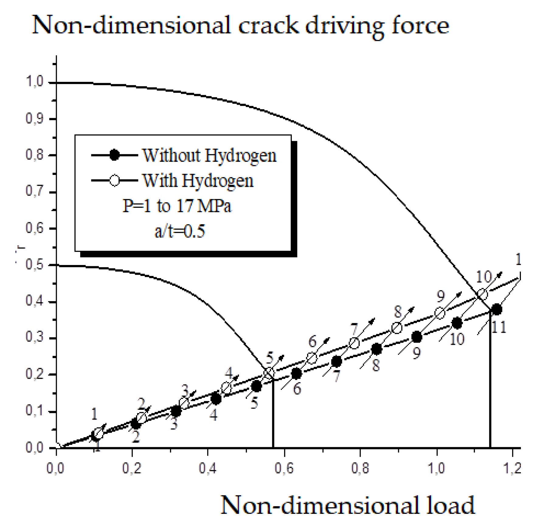
Reduction in fracture toughness by hydrogen embrittlement HE decreases with the non-dimensional crack driving force kr. Flow stress is not very affected by HE; therefore, it has practically no effect on non-dimensional load parameter.
A pipe subjected to internal pressure has a diameter D = 611 mm and thickness t = 11 mm. The pipe is damaged with an internal semi-elliptical crack. Crack characteristics are depth over thickness ratio a/t = 0.5 and aspect ratio a/c = 0.5.
Figure 14 shows that the loading path under HE is above the loading path without HE. After HE, the safety factor f
s is modified.
5.3. Influence of Hydrogen on the Safety Factor in FAD
According to Equation (13), safety factors have been computed. The studied pipe is submitted to internal pressure (
p = 5 and
p = 11 MPa). Five different values (a/t = 0.1, 0.2, 0.3, 0.4 and 0.5) of semi-elliptical defect sizes with identical aspect ratio is a/c = 0.5 are considered. When the defect becomes deeper, the safety factor decreases. Failure occurs only for the highest pressure (
p = 11 MPa) and for the deepest deep defects (a/t = 0.5 without HE and a/t = 0.4 with HE), see
Table 6.
6. Corrosion Defect Harmfulness after HE
A corrosion defect considered as semi-elliptical has the following dimensions: depth (a), length (2c) and, width (W). Failure emanating from this defect is controlled by its size and the flow stress of the material. Pipe outer diameter (D), wall thickness (t), specified minimum yield strength σ
y,
spc), the longitudinal extent of corrosion (2c) and, defect depth (d) are input parameters to compute the Maximum allowable Operating Pressure (MAOP). Limit pressure solutions for pipe with corrosion defects are proposed in codes and the literature (ASME B31G [
23], modified ASME B31G [
24], DNV RP-F101 [
25] and Choi et al. [
26]). The limit pressure
PL (
pl <
Pc the burst pressure) is expressed as:
Flow stress σ
0, α parameter and, Folias correction
M are different according to the applied method (see
Table 7).
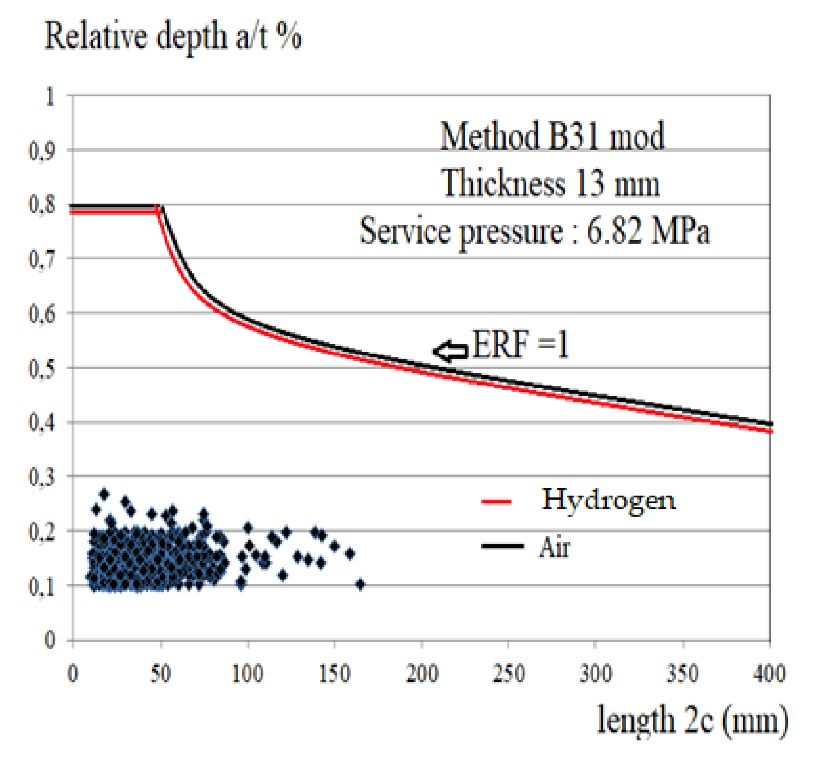
Using ASME B31G as defect assessment method allows calculating the safe operating pressure associated as the limit pressure. The ratio of the Maximum Allowable Operating Pressure (MAOP) and the safe operating pressure P
safe is the estimated repair factor ERF. The following criterion for repairing is:
Repairing or lowering MAOP is required if the ERF greater than one. The defect assessment point (2c*; a*/t) is reported in a graph of coordinates defect length, relative defect depth (2c; a/t),
Figure 15. The condition ERF = 1 is reported in this graph as a curve.
A defect is acceptable if its assessment point is below the ERF assessment curve. The assessment point above this curve requires repair or service pressure de-rating. An ERF assessment curve is specific to each method (B31 or B31 mod) through the computing of psafe or pL. These parameters depend on pipe diameter, thickness, and material flow stress σ0.
The linear loading path and the non-dimensional load axis are rotating from one angle called the assessment angle θ. Two values of the assessment angle can be defined θ. Two assessment angles determine three failure domains in the Domain Failure Assessment diagram (DFAD) diagram (
Figure 16):
- (i.)
If θ < θ1, it is localized the brittle fracture;
- (ii.)
If θ1 < θ < θ2, an elastoplastic fracture zone appears;
- (iii.)
If θ > θ2, the plastic collapses.
According to Federsen [
27], these zones are defined conventionally as follows:
where L
r,y is the non-dimensional yield pressure and L
r,max is a cut-off value. NFAD,
Figure 16, is used to choose the assessment method for failure risk evaluation for a pipe with a defect. For the pipe steel,
A pipe made from API 5L X52 steel with a corrosion defect is submitted to internal pressure. The pipe diameter is D = 611 mm and the thickness t = 11 mm t. This corrosion defect is considering as equivalent to an internal semi-elliptical crack (aspect ratio a/c = 0.5 and relative crack depth a/t = 0.5). Applied J integral is computed with the true stress/strain with and without HE of API 5L X52 pipeline steel.
From this applied J Integral
, the non/dimensional crack driving force is defined as:
where J
mat is the material fracture toughness. The loading path is presented in
Figure 17 (with and without HE).
The defect assessment (for a relative crack depth a/t = 0.1) is situated in the limit analysis domain when the material is not submitted to, HE. When submitted, the assessment point is situated in the LEFM domain.
In the LEFM domain, the safety factor is given by:
The safety factor for the limit analysis domain is defined as:
where p
l the limit pressure (according to ASME B31 [
23]) and
ps is the service pressure. In
Table 8, values of the safety factor for different relative defect depth ratios (a/t = 0.1 to 0.5), two different gas pressures as well hydrogen embrittlement are reported. F
s,
LA is calculated when the loading path is situated in the LA domain, i.e., for the relative defect depth a/t = 0.1; 0.2 and 0.3. The safety factors decrease when the applied pressure increases. HE induces a decrease in f
s by less than 10%. The safety factor associated with LA is always greater than the LEFM one. It decreases when the relative defect depth increases.
7. Strain-Based Design
Where loadings of pipelines are due to forces other than the internal pressure, strain-based design (SBD) is used. In this case, large stresses and strains in the pipe wall are produced.
When stresses and strains exceed the proportional limit SBD is rather used [
28,
29]. Stress-based methods are ruled by material stress–strain behavior. The strain-based design avoids these problems when strain and stress are not proportional. SBD is associated with limit states. Several limit states are considered with SBD: failure in tension (material limit state) and buckling by compression (material and serviceability limit states).
SBD fundamental equation is based on a comparison of the strain demand
and critical strain ε
cIn the absence of additional engineering information, a maximum strain limit of 10% (0.1) is considered. The safety factor f
s defines the critical strain capacity
:
where
εl is the limit strain. Safety factors according to the safety classes for tension are given in
Table 9. They are different for compression buckling. The difference between stress-based design and SBD is given in
Figure 18. The strain-based design of pipelines is described in several codes. DNV 2000 [
28] and CSA Z662 [
29] include requirements both for stress- and strain-based design. B31.8 [
30] and API 1104 [
31] incorporate strain-based design. API RP 1111 [
32] provides information on SBD related to a specific type of pipeline.
7.1. Influence of Loading Mode
The failure strain is sensitive to hydrostatic pressure σ
m and the Lode Angle,
θL. These parameters are considered in the Wierzbicki and Xue model [
33]. Failure strain is governed by the product of two specific functions associated with each parameter.
is the reference failure strain. The dependence with hydrostatic pressure
is given by:
if
if
q a material parameter
is the hydrostatic limit pressure. The dependence with the Lode angle is a power function as:
Dependence with Lode angle
is presented in polar coordinates.
γ is a material parameter. By increasing the values of
γ, one increases the influence of shear conditions on failure strain.
7.2. Influence of Hydrogen on Failure Elongation
Figure 19 shows for several pipe steels, the ratio of failure elongation under HE and without. One notes that the failure elongation ratio of A% (H2)/A% (air) decreases when the steel yield stress increases, however the scatter.
7.3. Application to Maximum Dent Depth after Hydrogen Embrittlement
Figure 20 shows a plain dent. A plain dent modifies the curvature of the pipe wall without reduction in pipe thickness. The distance between undamaged and damaged cross-sections defines the dent depth (
H). Plain dents have no sharp defects such as a gouge and possess a smooth profile.
For plain dents, it is necessary to consider the following parameters:
− Service pressure;
− Applied cyclic pressure range;
− Dent depth;
− Pipe geometry (ratio of diameter to wall thickness);
− Dent profile curvature.
Depth is the most significant factor affecting the burst strength and the fatigue life of a plain dent. The acceptability limits of dent depth are generally given by empirical rules. Depths up to 8% of pipe diameter [
34] do not significantly reduce the burst strength of a pipeline. The possibility of 24% [
35] exists for a plain smooth dent. Therefore, when dent depth is more than one-tenth of the pipe diameter, repairing is mandatory.
For the API 579 code [
36], dents are dangerous if they occur on longitudinal weld seams where cracks can develop. The European Pipeline Research Group (EPRG) [
37] indicates that dent depths up to 10% of the pipe outside diameter will not fail at membrane stress levels below 72% of the SMYS:
where
H = dent depth in the non-pressurized condition in (mm) and
De = pipe outside diameter (mm). The reduction in the dent depth by internal pressure (spring-back phenomenon) pushes out the dent. The measured depth must be corrected. EPRG found a correlation between the dent depth on a non-pressurized pipe and a pressurized pipe to be as follows [
37]:
where H
0 is the depth of the dent in the non-pressurized condition in (mm). According to EPRG, the dent depth limit in a pressurized pipe is [
37]:
A local strain criterion can be used to assess a dent This criterion assumes that the maximum local stress
has to be less than the failure strain ε
fThe Oyane et al. criterion [
38] is a local ductile failure criterion and written as follows:
where
is the equivalent failure strain;
σh the hydrostatic stress
the equivalent stress;
the equivalent deformation;
C1 and
C2 are material constants.
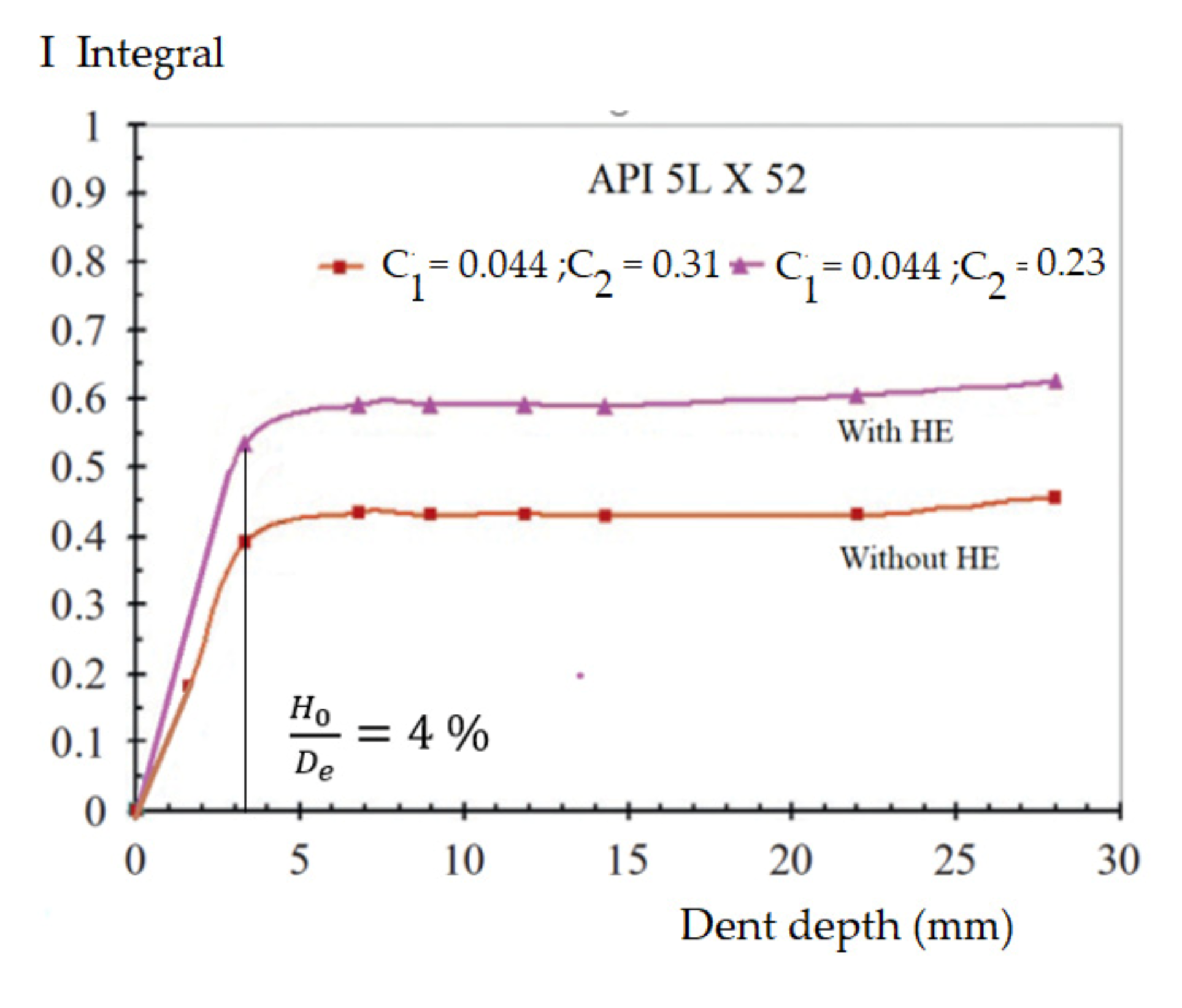
Oyane’s criterion is calculated for different dent depths. An example is given in
Figure 21 for a pipe made in API 5L X52 steel (failure elongation is 31.5% and after HE 23%). The results of calculations of I integral are related to material damage. One notes that this damage is much more severe when the steel is subjected to HE. After HE, the maximum damage is reached for a ratio
8. Conclusions
For transport of pure hydrogen or blended with natural gas, pipe design needs to consider the damage of pipe steels by hydrogen embrittlement.
The transition temperature is relatively low when compared with service temperature but are few affected by HE. Therefore, the reference temperature does not need to be modified.
The Maximum Admissible Operating Pressure (MAOP) needs to be modified through the design factor however the yield stress is few affected by HE. Therefore, the risk to human life is increased by the low ignition energy and large inflammability range of hydrogen.
HE strongly affects elongation at failure. Where loadings of the pipelines are due to forces other than the internal pressure, strain-based design (SBD) is used. This ensures that the strain demand remains less than strain capacity. These problems are partially covered in codes such as the ones in [
9].
Specific tools are necessary for pipe defect assessment (FAD, NFAD, ERF and damage criteria). They are specific to defect type (crack, gouge, corrosion crater or dent). These tools incorporate specific materials properties such as yield stress (low sensitivity to HE), fracture toughness, or failure elongation (very sensitive to HE). FAD, NFAD, ERF and damage criteris are recommended for a better defect assessment in pipes.


