Multi Set-Point Explicit Model Predictive Control for Nonlinear Process Systems

Abstract

In this article, we introduce a novel framework for the design of multi set-point nonlinear explicit controllers for process systems engineering problems where the set-points are treated as uncertain parameters simultaneously with the initial state of the dynamical system at each sampling instance. To this end, an algorithm for a special class of multi-parametric nonlinear programming problems with uncertain parameters on the right-hand side of the constraints and the cost coefficients of the objective function is presented. The algorithm is based on computed algebra methods for symbolic manipulation that enable an analytical solution of the optimality conditions of the underlying multi-parametric nonlinear program. A notable property of the presented algorithm is the computation of exact, in general nonconvex, critical regions that results in potentially great computational savings through a reduction in the number of convex approximate critical regions.

1. Introduction

High-fidelity and computationally efficient optimisation models are key for profitable decision making in process industries and have been the focus of extensive research over the years [1]. In recent years, the need for exploiting and explicitly considering interdependencies throughout the different layers of decision making has been underpinned by the enterprise-wide optimisation (EWO) concept [2]. Stemming from the progressively volatile and competitive market conditions, it is imperative for process industries to operate with agility in order to maximise their profitability [3]. EWO is aiming at increased profitability and resilience in process operations through the integration and simultaneous optimisation of existing information streams. Nonetheless, it comes at a considerable cost. Because of the multiple scales considered, EWO leads to computational challenges, thus preventing practitioners from harnessing the potential benefits such wide integration has to offer. Particularly, incorporating control considerations in an EWO fashion results in (mixed integer) nonconvex problems which are hard to solve.

By the same token, control considerations are ubiquitous in EWO problems. Figure 1 showcases how real-time optimisation and production scheduling exchange information with the layer of APC because of their interdependent decisions.

Real-time optimisation is concerned with the manipulation of systems’ dynamics in order to achieve optimised profitability and operations. On the other hand, production scheduling determines the optimal allocation of resources for the completion of competing tasks. As indicated by Figure 1, both RTO and process scheduling exchange information with the layer of APC so as to achieve optimal dynamic operations. To this end, the research community has proposed different methods for their integration.

A common shortfall when focusing on integrating RTO and APC is that two different models are employed for the optimisation of the same system. Typically, a locally linear model of the initial nonlinear dynamics is used at the APC because of the need for fast solution rates while RTO considers the original nonlinear model. This leads subsequently to issues related to suboptimal trajectories and non-reachable states [4].

Darby et al. [5], through their literature review regarding the integration of RTO and MPC, suggested that for a successful integration, common issues such as model mismatch among the layers of RTO and APC should be eliminated. Nonetheless, in real industrial processes, model degradation and other factors can result in model mismatch, so the consideration of parameter estimation and data reconciliation functionalities is needed to integrate RTO and MPC, as indicated by Figure 2.

The interaction between real-time optimisation and model predictive control can be categorised broadly into three classes: (i) dynamic RTO (d-RTO), (ii) static RTO (s-RTO) and (iii) economic model predictive control (e-MPC). Both s-RTO and d-RTO are two-layer schemes where reference trajectories are passed to the layer of APC in the form of set-points [6]. While under the static real-time optimisation paradigm, the optimisation problem is solved at specific instances whenever new data become available or when steady state is achieved, in the d-RTO paradigm, the system’s transient behaviour is explicitly considered, thus resulting in dynamic optimisation problems. e-MPC [7] refers to single-layer strategies which are incorporated into the control structure economic considerations. In that spirit, De Souza et al. [8] proposed the inclusion of the gradient of the economic objective function into the MPC objective as a single-layer strategy. Considering uncertain systems, Chachuat et al. [9] examined alternative model adaptation strategies.

This article is motivated by the abovementioned issues and aims at introducing a method for designing multi set-point explicit controllers for nonlinear systems through recent advances in multi-parametric programming. Multi-parametric programming (mp-P) has received considerable attention from the process systems engineering community because of its unique ability to aid in the design of explicit model predictive controllers and thus shift the computational burden associated with offline control [10]. We examine a case of multi-parametric nonlinear programs (mp-NLPs) that involve both endogenous uncertainty, in the form of left-hand side parameters (LHS), as well as exogenous uncertainty in the cost coefficient of the objective function (OFC), and, on the right-hand side of the constraints (RHS), uncertain parameters on the right-hand side (RHS). In engineering problems, LHS uncertainty arises from variations in model coefficients, due to parameter estimation errors or model mismatch; OFC uncertainty arises due to fluctuation in market prices or control penalties while RHS uncertainty can be due to varying system exogenous factors. The contribution of the present work is a novel framework for the design of multi set-point explicit controllers for nonlinear process systems.

The remainder of the article is organised as follows: in Section 2, an overview of the field of multi-parametric programming and explicit MPC is given, and then, in Section 3, the proposed algorithm is detailed and a framework for multi set-point explicit controllers is introduced. In Section 4, two case studies are examined so as to illustrate the main computational steps of the proposed methodology and, lastly, in Section 5, concluding remarks are made.

2. Background

2.1. Multi-Parametric Programming

Overall, multi-parametric programming problems are concerned with the effect of parametric perturbations on the optimal solution of an optimisation problem. Consider the following optimisation problem:

$$\begin{array}{c}\begin{array}{ccc}z\left(\mathbf{\theta }\right)=& \underset{\mathbf{x}\in {\mathbb{R}}^{n_x}}{\min }& f(\mathbf{x},\mathbf{\theta })\\ & \mathrm{subject}\mathrm{to}:& \mathbf{g}(\mathbf{x},\mathbf{\theta })\le 0\\ & & \mathbf{\theta }\in {\mathbb{R}}^{n_{\theta }}\end{array}\end{array}$$

(1)

where $\mathbf{\theta }$ stands for the vector of uncertain parameters, which is $n_{\theta }$-dimensional, $\mathbf{x}$ is the $n_x$-dimensional vector of continuous decision variables, $\mathbf{g}(\mathbf{x},\mathbf{\theta })$ is the vector of inequality constraints and f is the objective function as a mapping ${\mathbb{R}}^{n_x\times n_{\theta }}\to \mathbb{R},$ both of which are assumed to be ${\mathcal{C}}^2$ (twice continuously differentiable). 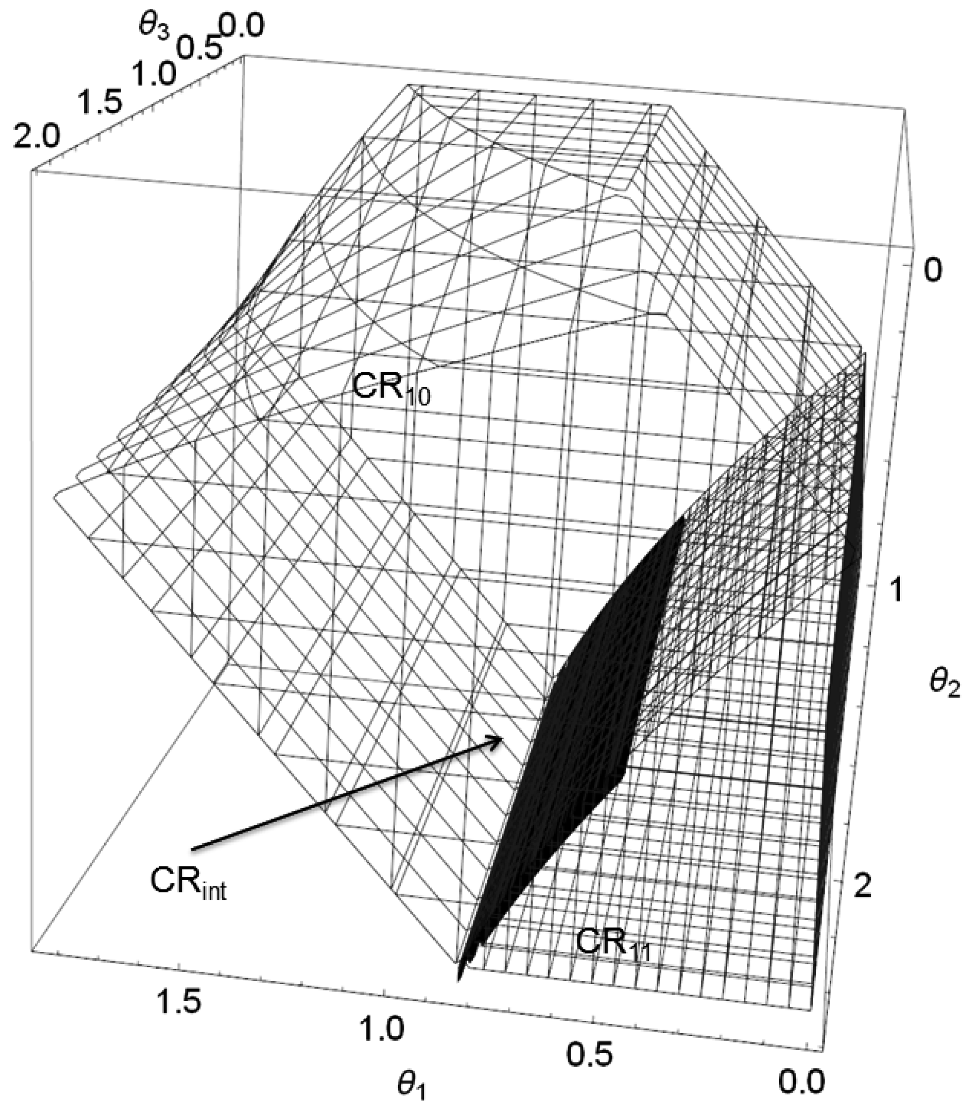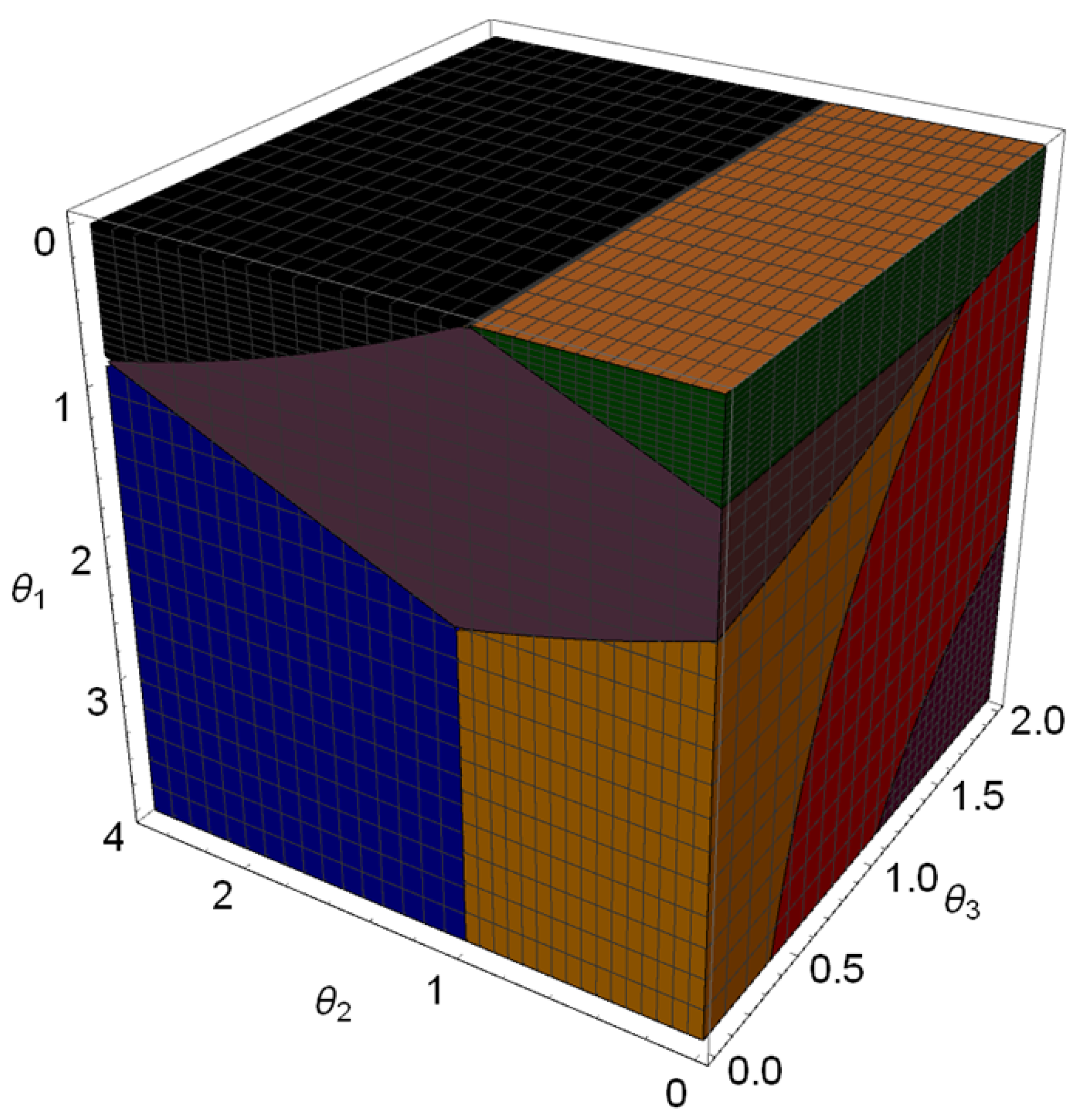Problem (1) is a multi-parametric program and its solution results in the partition of the parametric ${\mathbb{R}}^{n_{\theta }}$-space into a number of regions, also know as critical regions (CRs). Within each CR, the optimal solution and the objective value are given as functions of the uncertain parameters, i.e., $\mathbf{x}\left(\mathbf{\theta }\right)$ and $\mathbf{z}\left(\mathbf{\theta }\right)$, respectively. Even though mp-P has been studied quite actively, the class of multi-parametric nonlinear programming problems remains one of the most challenging ones [11,12]. Depending on the convexity of the nonlinear functions that form Problem (1), different solution techniques have been proposed in the literature to date.

Advances in the algorithms and theory of parametric nonlinear programs (p-NLPs) date back to the early works of Fiacco [13] and Bank et al. [14]. More specifically, in the books of Bank et al. [14] and Fiacco [13], a collection of the early research works for parametric NLPs can be found and invaluable theoretical foundations for some classes of convex p-NLPs with perturbations in the OFC and the right-hand side of the constraints are provided. Even though the term “parametric nonlinear optimisation/programming” was widely established from the aforementioned works, the early works on numerical stability analysis of NLPs by [15,16] and the work of Robinson [17,18] on generalised equations provided a significant way of studying the effect of parametric variations on the optimal solution of p-NLPs. Kyparisis [19] studied the uniqueness and differentiability of solutions of parametric nonlinear complementarity problems while in Ralph and Dempe [20], the directional derivatives of parametric nonlinear programs were used to characterise their explicit solution. However, the first algorithm for the multi-parametric case of convex NLPs was due to Dua and Pistikopoulos [21]. The authors, based on the findings about the convexity properties of the parametric value function ($z\left(\mathbf{\theta }\right)$), devised an iterative procedure in which the integer variables were fixed by the solution of a primal mixed integer nonlinear program (MINLP) and the resulting mp-NLP was then transformed into an mp-LP following the outer approximation idea. Because of the value function’s convexity property, the maximum error of the approximation occurs at the vertices of the CRs and if the error is greater than the prespecified tolerance, the CR is partitioned again; otherwise, integer and parametric cuts are implemented and then the algorithm iterates until the primal MINLP is infeasible. The same algorithm was revisited by Acevedo and Salgueiro [22], where the authors proposed heuristics to improve its computational efficiency while quadratic approximations were studied by Johansen [23] and Domínguez and Pistikopoulos [24]. An approximate algorithm for the solution of convex mp-NLPs was proposed by Johansen [25], who proposed the consecutive subdivision of the parametric space in hyper-rectangles and the interpolation of the parametric solution through the solution of $2^{n_{\theta }}$ NLPs at each step. Further approaches involve the geometric vertex search by Narciso [26] and sub-gradient methods by Leverenz et al. [27]. For the nonconvex cases, Dua et al. [28] developed suitable parametric under/overestimators which were then incorporated into a spatial branch and bound routine for the global optimisation of the nonconvex problem within $ϵ$—tolerance. For a more thorough discussion on the algorithms that have been proposed for the solution of mp-NLPs, the interested reader is directed to the review of Domínguez et al. [29] while Hale [30], in her doctoral thesis, also offers a thorough discussion on several classes of parametric optimisation. Fotiou et al. [31,32] initially studied the polynomial multi-parametric programming problem with application to control, however, their approach did not include the definition of final nonconvex CRs, while the mixed integer polynomial case was studied by Charitopoulos and Dua [33] and a procedure for the computation of exact nonconvex CRs was presented. Despite the aforementioned research effort, mp-NLP problems remain one of the most difficult to tackle and, as illustrated in

Table 1. Summary of multi-parametric nonlinear programmming algorithms.

mp-NLP Solution Techniques	RHS	LHS	OFC	Comments
Dua and Pistikopoulos [21]	√	-	-	Convex
Johansen [23]	√	-	-	Convex
Acevedo and Salgueiro [22]	√	-	-	Convex
Johansen [25]	√	-	-	Convex
Dua et al. [28]	√	-	-	Nonconvex
Fotiou et al. [31]	√	-	-	Polynomial
Narciso [26]	√	-	-	Convex
Domínguez and Pistikopoulos [24]	√	-	-	Convex
Charitopoulos and Dua [33]	√	-	-	Polynomial
Pappas et al. [34]	√	-	-	QCQPs

, all the aforementioned algorithms can handle uncertain parameters only on the right-hand side (RHS) of the constraints. Recently, Pappas et al. [34], by generalising the basic sensitivity theorem of Fiacco [13], devised an algorithm for the exact solution of multi-parametric quadratically constrained quadratic programs.

Among the wide range of appplications that multi-parametric programming has been applied to, the invention of explicit model predictive control (mp-MPC) is undoubtedly the most dominant area where mp-P has had the biggest impact [10,12,35]. The main concept of mp-MPC is that instead of solving the optimisation problems related to standard MPC at each sampling instance, the state of the system is treated as an uncertain parameter and an mp-P can be solved offline to derive the explicit control solution once and for all [10,36].

The general formulation of mp-MPC for discrete time systems is shown by (2):

$$\begin{array}{c}(mp-MPC)\left\{\begin{array}{cc}& \Phi \left(x\left(t_k\right)\right)=\underset{\mathbf{u}}{\min }{\displaystyle \sum _{i=0}^{P_H-1}}\mathcal{L}(x_t,u_t)+E\left(x_N\right)\hfill \\ & \mathrm{subject}\mathrm{to}:x_{t|t=0}=x\left(t_k\right)\hfill \\ & x_{t+1}=f(x_t,u_t)t=0,1,\dots ,P_H-1\hfill \\ & y_{t+1}=h(x_t,u_t)t=0,1,\dots ,P_H-1\hfill \\ & \mathbf{A}{x}_t\le \mathbf{\alpha }t=0,1,\dots ,P_H\hfill \\ & \mathbf{B}{y}_t\le \mathbf{\beta }t=0,1,\dots ,P_H\hfill \\ & \mathbf{C}{u}_t\le \mathbf{\gamma }t=0,1,\dots ,P_H\hfill \end{array}\right.\end{array}$$

(2)

where ${\mathbf{x}}_t,{\mathbf{u}}_t,{\mathbf{z}}_t$ are the state, control input and system output vectors, respectively, at every sampling point, t, and are $n_x,n_u,n_y$-dimensional. $\mathbf{A},\mathbf{B},\mathbf{C}$ are matrices of appropriate dimensions and $\mathbf{\alpha },\mathbf{\beta },\mathbf{\gamma }$ vectors of pertinent dimensions which represent inequality constraints for the state, output and control inputs while $\mathcal{L}:{\mathbb{R}}^{n_x+n_u}\to \mathbb{R}$ is a stage cost and $E:{\mathbb{R}}^{n_x}\to \mathbb{R}$ is a terminal cost function. The repetitive solution of Problem (2) provides the optimal cost $\Phi \left(\mathbf{x}\left(t_k\right)\right)$ and the optimisation vector, i.e., the sequence of optimal control inputs ${\mathbf{u}}^{*}=\left[{\mathbf{u}}_1^{*},{\mathbf{u}}_2^{*},\dots ,{\mathbf{u}}_{P_H-1}^{*}\right]$ over the finite prediction horizon $P_H$. Compared to the conventional model predictive control fashion, in which an optimisation problem is solved at each sampling point, through the mp-MPC notion, the explicit control law is calculated offline once and for all. The solution of the resulting mp-P problem results in the optimal control inputs as explicit functions of the (uncertain) parameters, i.e., the state of the system at each sampling instance, along with the corresponding CRs, as shown by Equation (3).

$$\begin{array}{c}{\mathbf{u}}^{*}=\left\{\begin{array}{cc}{\nu }_1\left(\mathbf{x}\left({\mathbf{t}}_{\mathbf{k}}\right)\right)\hfill & if\mathbf{x}\left({\mathbf{t}}_{\mathbf{k}}\right)\in C{R}_1\hfill \\ {\nu }_2\left(\mathbf{x}\left({\mathbf{t}}_{\mathbf{k}}\right)\right)\hfill & if\mathbf{x}\left({\mathbf{t}}_{\mathbf{k}}\right)\in C{R}_2\hfill \\ ⋮\hfill & ⋮\hfill \\ {\nu }_{\omega }\left(\mathbf{x}\left({\mathbf{t}}_{\mathbf{k}}\right)\right)\hfill & if\mathbf{x}\left({\mathbf{t}}_{\mathbf{k}}\right)\in C{R}_{\omega }\hfill \end{array}\right.\end{array}$$

(3)

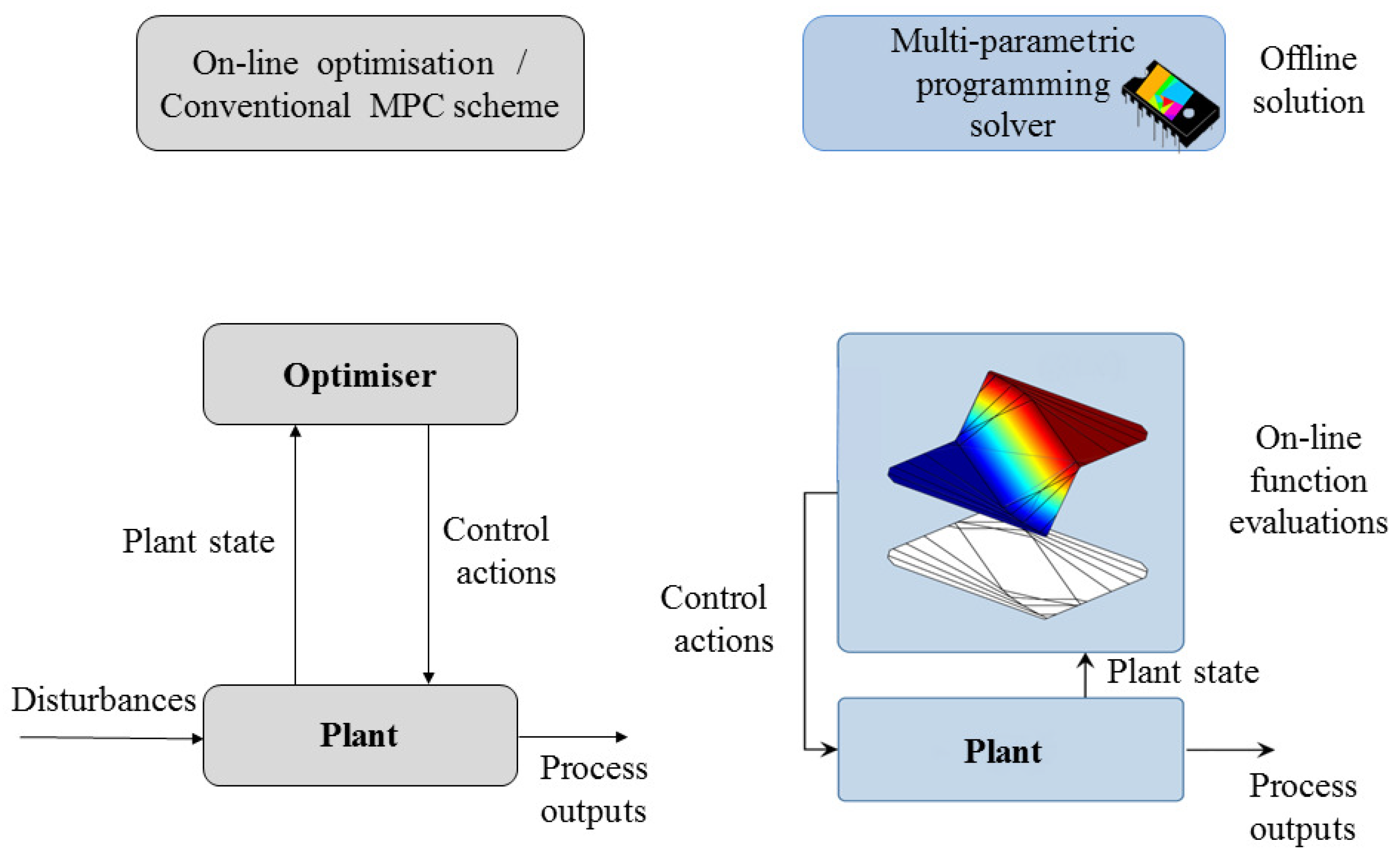
For the case of MPC for linear systems, instead of solving a quadratic program at each sampling instance, the explicit MPC requires the offline solution of an mp-QP while online, so only simple function evaluations are required [10,37,38]. This concept is also known as online via offline optimisation and it is shown in Figure 3.

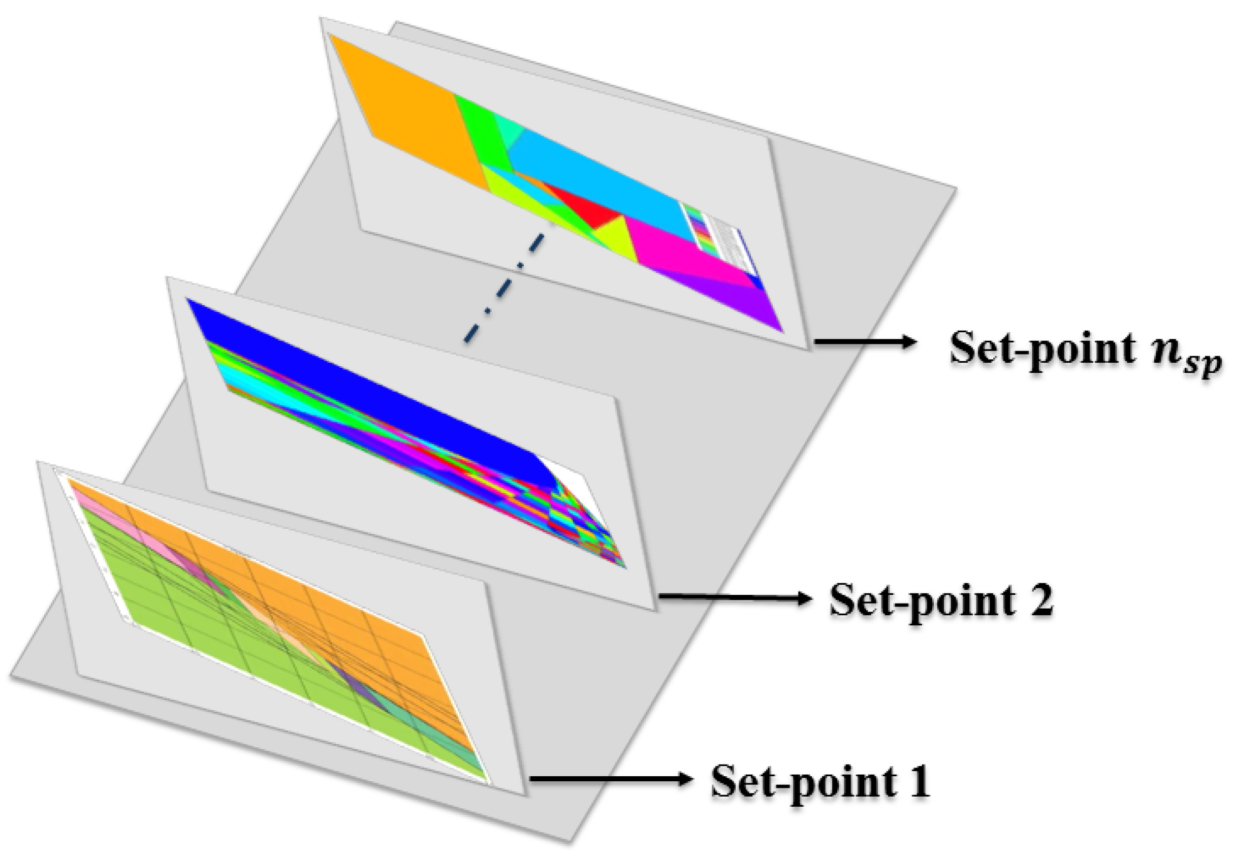
Even though mp-MPC is the niche area of mp-P, designing mp-MPCs of nonlinear systems for set-point tracking is still a computationally strenuous task as one has to design an mp-MPC for each set-point based on the algorithms that exist in the literature to date [40]. Next, we review two mathematical techniques that will enable the development of novel multi set-point explicit controllers though the algorithm we propose in the present work.

2.2. Computer Algebra

2.2.1. Gröbner Bases Theory

The idea of the present work is to devise an algorithm for the solution of mp-NLPs from an analytical and not numerical perspective, and the reason is two-fold. Firstly, for the case that we are interested in, i.e., mp-NLPs with combined uncertainty on the RHS and OFC, no theoretical foundations exist for the computation of the explicit solution like the basic sensitivity theorem of Fiacco [13] which serves as the basis of the numerical mp-P approaches. Secondly, because of the nonconvex nature of the parametric problem, the numerical solution would require global optimisation techniques similar to the ones presented in Dua et al. [28] and would lead to an explosion in the number of convex approximate CRs.

Gröbner bases theory was introduced by the doctoral research of Bruno Buchberger [41] as a method of analytically solving systems of multivariate polynomial equations. In brief, Gröbner bases and the Buchberger algorithm can be considered as the polynomial counterpart of Gaussian elimination for the case of nonlinear systems. Before formally defining what a Gröbner basis is, it would be useful to define some preliminary concepts.

Definition 1.

Power products

Let $\mathbb{R}$ be any field and let $\mathbb{R}[x_1,\dots ,x_n$] be the ring of polynomials in n-indeterminates. Any polynomial can be described as a sum of terms of the form: $\alpha x_1^{{\beta }_1}\cdots x_n^{{\beta }_n}$ with $\alpha \in \mathbb{R}$ and ${\beta }_i\in \mathbb{N},i=1,\dots ,n$ and the term $x_1^{{\beta }_1}\cdots x_n^{{\beta }_n}$ is called a power product.

Definition 2.

Term order

A term order is defined with regard to a set of power products ($T_n$) and imposes a total order < on the set in compliance with the conditions below:

1. 

$1<x^{\beta }$ for all $x^{\beta }\in T_n$

2. 

If $x^{\alpha }<x^{\beta }\to x^{\alpha }{x}^{\gamma }<x^{\beta }{x}^{\gamma }$, for all $x^{\gamma }\in T_n$

A number of alternative power product orderings exist but the most commonly employed is the the lexicographic one due to its computational efficiency [42]. Lastly, the notion of ideals is crucial within the Gröbner bases theory.

Definition 3.

Ideals

Let $\mathbb{R}$ be a field and $\mathbb{R}[x_1,x_2,\dots ,x_n]$ be a ring over the field of n-variate polynomials. Let a finite subset of the field, $G=\{g_1,g_2,\dots ,g_t\}$, then an ideal I can be generated by G as follows:

$$\begin{array}{ccc}\hfill I& =& \{\sum _{i=1}^n{u}_i{g}_i|u_i\in \mathbb{R}[x_1,x_2,\dots ,x_n],g_i\in \mathbb{R},\forall i\hfill \end{array}$$

For problems that accept analytical solutions, their existence is guaranteed by the Hilbert basis theorem [43], which also guarantees that algorithms used to compute Gröbner bases can terminate in a finite number of steps.

Definition 4.

$Gröbner$ basis [41]

A set of non-zero polynomials $G=\{g_1,\dots ,g_t\}$, contained in an ideal I, is called a $Gröbner$ basis for I if and only if for all $g\in I$, such that $g\ne 0$, there exists $i\in \{1,\dots ,t\}$ such that $lp(g_i)$ divides $lp\left(g\right)$, where $lp(·)$ stands for the leading power product of a polynomial function.

For the calculation of Gröbner bases, apart from Buchberger’s algorithm, Faug$\mathrm{è}$re has presented algorithms F4 [44] and F5 [45] as two variants of another algorithm. They exploit concepts from linear algebra and represent polynomials using matrix forms, thus enabling successive truncated Gröbner bases to be created. Lastly, software implementations of different algorithms that compute Gröbner bases computations can be found in freely available CAS such as Singular, SymPy and SageMath as well as commercial tools like Maple and Mathematica.

2.2.2. Cylindrical Algebraic Decomposition (CAD)

The notion of cylindrical algebraic decomposition was presented by Collins in 1975 [46] in an effort to solve the problem of quantifier elimination over real closed fields. In this article, as will be shown later on, CADs are used for computing nonconvex regions in the space of parameters. Thus, we provide the following definitions for ease of exposition in the algorithmic steps that we detail later on in the manuscript.

Definition 5.

Semi-Algebraic Sets [43].

Let $\mathbb{R}[x_1,x_2,\dots ,x_n]$ indicate the ring of polynomials in n-indeterminates with real coefficients. If, for example, a subset $\mathcal{S}$ of ${\mathbb{R}}^n$ can be developed by a finite number of applications of the complementation, union and intersection operations, it is called semi-algebraic and can have the following form:

$\{\mathbf{x}\in {\mathbb{R}}^n|\mathbf{g}\left(\mathbf{x}\right)\le 0\}$, where $\mathbf{g}\in \mathbb{R}\left[X\right]$

Definition 6.

Standard atomic formula

A formula that includes a functional relation over a polynomial ring in either of the ways shown below is called a standard atomic formula:

$$\begin{array}{c}g\left(\mathbf{x}\right)=0,g\left(\mathbf{x}\right)\ne 0,g\left(\mathbf{x}\right)<0,g\left(\mathbf{x}\right)>0,g\left(\mathbf{x}\right)\le 0,g\left(\mathbf{x}\right)\ge 0\end{array}$$

Proposition 1

([43]). Semi-algebraic sets of ${\mathbb{R}}^n$ can be written as a finite union of semi-algebraic sets of the form:

$$\begin{array}{c}\{\mathbf{x}\in {\mathbb{R}}^{n_X}|g_1\left(\mathbf{x}\right)=\dots =g_{\omega }\left(\mathbf{x}\right)=0,g_{\omega +1}\left(\mathbf{x}\right)>0,\dots ,g_t\left(\mathbf{x}\right)>0\}\end{array}$$

where $g_1\dots ,g_{\omega },g_{\omega +1},\dots ,g_t$ are in $g\in \mathbb{R}\left[X\right]$.

The proof of the proposition can be found in the book of Bochnak et al. [43].

Using the definitions and propositions given above, in summary, one can use CAD routines to compute the solution to polynomial inequalities. In the process of computations, one partitions the related space over finite cells and qualifies whether or not standard atomic formulas hold. A comprehensive exposition on the solution of polynomial inequalities using CAD is given at the book of Jirstrand [47].

3. Algorithms and MPC

3.1. Multi Set-Point Explicit Controller via Multi-Parametric Programming

In the context of multi-parametric model predictive control, the state of the system at each sampling point is treated as an uncertain parameter and as a result an mp-P with RHS uncertainty arises [10,37,38,40]. Its solution results in the explicit control law, i.e., the control decisions as explicit functions of the system’s initial conditions at a sampling instance along with the related CRs.

In many applications, however, particularly those related to continuous manufacturing, there is a great need for fast calculations in order to communicate decisions between the different layers of decision making in an effective manner. For instance, set-point tracking goals for APC are, most of the time, passed down from either the functionality of process scheduling or RTO [39,48]. In these cases, it becomes obvious that explicit MPC can provide a significant advantage in computational time by treating the set-points or estimated model inputs as uncertain parameters. One way to design such explicit controllers, assuming the existence of the $n_u$ set-point, is to solve $n_u$ mp-P problems and thus design $n_u$ mp-MPCs. Another way, which has not been investigated in the literature, is to consider the set-points and/or model inputs as uncertain parameters and thus derive a multi set-point explicit MPC. Conceptually, by doing so, we would design a layered controller as given by Figure 4.

Conventionally, when mp-MPC is employed for set-point tracking of nonlinear systems, one would have to compute a different mp-MPC for each of those set-points as well as account for any time delay in the offline solution of the related mp-P should a new set-point arise. Stringent market regulations and an increasingly volatile market environment lead process industries to constantly optimise their operations and give rise to new set-points from a control perspective which in turn hinder the deployment of mp-MPC. As illustrated by Figure 4, in this article, by considering the set-points as uncertain parameters which lie within prespecified bounds, we overcome the abovementioned drawback of explicit MPC since, by solving one mp-NLP, we can design a “multi set-point” mp-MPC for nonlinear systems.

The design problem of a multi set-point mp-MPC can be formulated as in (4).

$$\begin{array}{c}\left\{\begin{array}{cc}& {\rm Y}(x\left(t_k\right),x_{sp})=\underset{\mathbf{u}}{\min }{\displaystyle \sum _{t=0}^{P_H-1}}\mathcal{L}(x_t,u_t,x_{sp})+E(x_N,x_{sp})\hfill \\ & \mathrm{subject}\mathrm{to}:x_{t|t=0}=x\left(t_k\right)\hfill \\ & x_{t+1}=f(x_t,u_t)t=0,1,\dots ,P_H-1\hfill \\ & y_{t+1}=h(x_t,u_t)t=0,1,\dots ,P_H-1\hfill \\ & \mathbf{A}{x}_t\le \mathbf{\alpha }t=0,1,\dots ,P_H\hfill \\ & \mathbf{B}{y}_t\le \mathbf{\beta }t=0,1,\dots ,P_H\hfill \\ & \mathbf{C}{u}_t\le \mathbf{\gamma }t=0,1,\dots ,P_H\hfill \\ & x_{sp}\in {\mathbb{R}}^{n_{sp}}\hfill \end{array}\right.\end{array}$$

(4)

The notation adopted is the same as in the previous section, aside from the following: we treat the set-points together with the initial state of the system as uncertain parameters, thus resulting in a problem with simultaneous variations on the RHS and OFC. As indicated by (4), we consider both the initial states ($x\left(t_k\right)$) and the various set-points ($x_{sp}$) as uncertain parameters. Notice that within an EWO framework, the deployment of such universal controllers is of great importance since they allow for rapid communication between the layer of control with RTO and scheduling. For instance, when integrating scheduling with control, the changeover times as well as the production rates are immediate results of the dynamic decisions made through the control system. In the next section, an algorithm for the design of such “multi set-point” explicit MPC is presented.

3.2. Solution Algorithm for Analytical mp-NLPs with Global Uncertainty

Here, we present an algorithm that can solve multi-parametric nonlinear programs with non transcendental nonlinear terms, i.e., nonlinear terms that have closed-form solutions. The proposed method can be seen as a generalisation of the our previous work on the solution of multi-parametric mixed integer polynomial programs [33] as well as the algorithm of Fotiou et al. [32] for multi-parametric polynomial programs. However, both of these methods were employed only for instances that the uncertainty is present on the right-hand side of the constraints and the latter does not compute the critical regions associated with each explicit solution.

The main idea of the algorithm proposed herein can be explained as follows: given a multi-parametric nonlinear program with analytical terms, or terms that can be expressed in a nontranscendental fashion, derive the first order KKT conditions and compute its solution using Gröbner bases by treating the uncertain parameters as symbols. The output of this step is a collection of candidate solutions which are explicit in $\mathbf{\theta }$ and encompass: global and local optima as well as infeasible solutions. For these solutions, examine their dual and primal feasibility along with a constraint qualification so as to remove infeasible candidate solutions. Lastly, in order to report only the globally optimal solutions, perform a comparison procedure [33].

Problem (1) details a general formulation of multi-parametric programs. The case that f and/or $\mathbf{g}$ are analytically nonlinear and the uncertain parameters are in the OFCs along with the RHS and LHS of the constraints is used.

Deriving the 1st order KKT conditions of Problem (1) returns a system of equations that is square and is given by Equations (5) and (6).

$$\begin{array}{c}{\nabla }_{\mathbf{x}}L(\mathbf{x},\mathbf{\theta })=\mathbf{0}\end{array}$$

(5)

$$\begin{array}{c}{\lambda }^T\mathbf{g}(\mathbf{x},\mathbf{\theta })=\mathbf{0}\end{array}$$

(6)

$L(\mathbf{x},\mathbf{\theta })$ is the Lagrangian function of Problem (1), ${\nabla }_{\mathbf{x}}$ is the nabla operator with respect to the decision variables and $\mathbf{\lambda }$ are the Lagrange multipliers corresponding to the constraints. Because of the assumption that the nonlinearities have an analytical solution, Gröbner bases can be employed for the solution of the square system of equations because of its elimination property. Even though a tailored implementation of one of the already existing algorithms for computing Gröbner bases may be advantageous from a computational standpoint, it is beyond the scope of the present work and thus Mathematica 10 was employed as the computer algebra software in which the calculations were performed.

By solving the system of Equations (5) and (6), a number of candidate solution sets are returned. Note that although the original optimisation problem involves $n_x$ variables, in the current step, the variables for which we compute the explicit solution are $n_x+n_g$. The candidate solutions include the Lagrange multipliers together with the optimisation variables as explicit functions of the uncertain parameters, i.e., $\mathbf{\lambda }\left(\mathbf{\theta }\right)$ and $\mathbf{x}\left(\mathbf{\theta }\right)$, respectively.

Definition 7.

Candidate solutions [49]

A solution of the Problem (1) is said to be candidate if it satisfies the system of Equations (5) and (6) along with a constraint qualification, e.g., linear independence constraint qualification [15].

In this part of the algorithm, due to strict complementary slackness, the collection of candidate solutions indicates the active and inactive constraints for each solution. Until this step, the set of solutions computed may be infeasible, local or global optima. By evaluating the primal and dual feasibility of the candidate solutions, the infeasible solutions can be rejected, i.e., Equations (7) and (8).

$$\begin{array}{c}\mathbf{g}\left(\mathbf{\theta }\right)\le \mathbf{0}⟹feasibilityconditions\end{array}$$

(7)

$$\begin{array}{c}\mathbf{\lambda }\left(\mathbf{\theta }\right)\ge \mathbf{0}⟹optimalityconditions\end{array}$$

(8)

Conditions (7) and (8) are evaluated by substituting the explicit expressions of the optimisation variables and they form a collection of parametric constraints. If for a candidate solution there exists a subset of the initial parametric space such that the aforementioned inequalities are satisfied, then this region is called the CR of the candidate feasible solution; otherwise, the candidate solution is infeasible and thus removed from further consideration. Note that the evaluation performed at this step, from a computer algebra perspective, is equivalent to computation of the corresponding CAD.

Definition 8.

Critical region [39,49]

A critical region (CR) is a partition of the parametric space where Conditions (7) and (8) are satisfied for a specific candidate solution. A critical region is characterised by a set of inactive/active constraints and can be discontinuous or nonconvex.

In Algorithm 1, the pseudo-code of the presented method is given. The comparison procedure is outlined in [33].

3.3. Illustrative Example

The proposed methodology will be motivated through the following modified example by Domínguez et al. [29].

$$\begin{array}{c}\underset{x_{1,}{x}_2}{min}x+2x_1^2-5x_1+x_2^2-3{\theta }_1{x}_2-6\end{array}$$

Subject to:

$$\begin{array}{c}2x_1+x_2\le 2.4-{\theta }_2\\ 0.5{\theta }_3{x}_1+x_2\le 1.5\\ x_1\ge 0,x_2\ge 0\\ 0\le {\theta }_1\le 6,0\le {\theta }_2\le 4,0\le {\theta }_3\le 2\end{array}$$

(9)

In the beginning, the first order KKT conditions of (9) are formulated and we derive the square system of Equations (10) and (14)

$$\begin{array}{c}{\nabla }_{\mathbf{x}}L(\mathbf{x},\mathbf{\lambda },\mathbf{\theta })=\mathbf{0}\end{array}$$

(10)

$$\begin{array}{c}{\lambda }_1(2x_1+x_2-2.5+{\theta }_2)=0\end{array}$$

(11)

$$\begin{array}{c}{\lambda }_2(0.5{\theta }_3{x}_1+x_2-1.5)=0\end{array}$$

(12)

$$\begin{array}{c}{\lambda }_3(-x_1)=0\end{array}$$

(13)

$$\begin{array}{c}{\lambda }_4(-x_2)=0\end{array}$$

(14)

where $L(\mathbf{x},\mathbf{\lambda },\mathbf{\theta })$ is the Langangian of Problem (9). Equations (10) and (14) can be analytically solved through symbolic computations which return the dual and primal variables as functions of the uncertain parameters, i.e., $\mathbf{\lambda }\left(\theta \right)$ and $\mathbf{x}(\mathbf{\theta })$. Systems (10)–(14) are solved in 0.006 s and, as shown in

Table A1. Candidate solutions of motivating example.

	${\mathit{x}}_1$	${\mathit{x}}_2$	${\mathbf{\lambda }}_1$
1	−2.12	0	0
2	−2.12	$1.5{\theta }_1$	0
3	0	1.5	0
4	0	$0.5(5-2{\theta }_2)$	$3{\theta }_1+2{\theta }_2-5$
5	0	0	0
6	0	$1.5{\theta }_1$	0
7	0.786	0	0
8	0.786	$1.5{\theta }_1$	0
9	$-0.577\sqrt{-6{\theta }_1-4{\theta }_2+27}-2$	$0.5\left(2.309\sqrt{-6{\theta }_1-4{\theta }_2+27}-2{\theta }_2+13\right)$	$0.333\left(-6.9282\sqrt{-6{\theta }_1-4{\theta }_2+27}+9{\theta }_1+6{\theta }_2-39\right)$
10	$0.333\left(1.732\sqrt{-6{\theta }_1-4{\theta }_2+27}-6\right)$	$0.166\left(-6.928\sqrt{-6{\theta }_1-4{\theta }_2+27}-6{\theta }_2+39\right)$	$2.309\sqrt{-6{\theta }_1-4{\theta }_2+27}+3{\theta }_1+2{\theta }_2-13$
⋮	⋮	⋮	⋮
14	$0.0833\left(-\sqrt{{\theta }_3^4-72{\theta }_1{\theta }_3+16{\theta }_3^2+72{\theta }_3+304}-{\theta }_3^2-8\right)$	$0.0416\left({\theta }_3\sqrt{{\theta }_3^4-72{\theta }_1{\theta }_3+16{\theta }_3^2+72{\theta }_3+304}+{\theta }_3+8{\theta }_3+36\right)$	0
15	$0.0833\left(\sqrt{{\theta }_3^4-72{\theta }_1{\theta }_3+16{\theta }_3^2+72{\theta }_3+304}-{\theta }_3^2-8\right)$	$0.0416\left(-{\theta }_3\sqrt{{\theta }_3^4-72{\theta }_1{\theta }_3+16{\theta }_3^2+72{\theta }_3+304}+{\theta }_3+8{\theta }_3+36\right)$	0
	${\lambda }_2$	${\lambda }_3$	${\lambda }_4$
1	0	0	$-3{\theta }_1$
2	0	0	0
3	$3({\theta }_1-1)$	$0.5(3{\theta }_1{\theta }_3-3{\theta }_3-10)$	0
4	0	$6{\theta }_1+4{\theta }_2-15$	0
5	0	−5	$-3{\theta }_1$
6	0	−5	0
7	0	0	$-3{\theta }_1$
8	0	0	0
9	0	0	0
10	0	0	0
⋮	⋮	⋮	⋮
14	$0.0833(-{\theta }_3\sqrt{{\theta }_3^4-72{\theta }_1{\theta }_3+16{\theta }_3^2+72{\theta }_3+304}+36{\theta }_1-{\theta }_3^3-8{\theta }_3-36)$	0	0
15	$0.0833({\theta }_3\sqrt{{\theta }_3^4-72{\theta }_1{\theta }_3+16{\theta }_3^2+72{\theta }_3+304}+36{\theta }_1-{\theta }_3^3-8{\theta }_3-36)$	0	0

, fifteen candidate solutions are computed.

The primal and dual feasibility of the candidate solutions is examined by computing the CAD of the related disjunctions. If the result of this step is “False” the solution violates feasibility (in either the primal or dual sense), otherwise, a collection of explicit inequalities is returned which characterises the candidate solution’s CR. The CAD computations of this example take 5.33 s and nine of them are nonempty. Despite the fact that nine candidate solutions are primal and dual feasible, their global optimality is not guaranteed given the nonconvex nature of the problem. To this effect, for those regions, a new set of CAD computations is performed so as to identify overlaps.

Algorithm 1: mp-NLP under global uncertainty

It was found that $C{R}_{10}$ and $C{R}_{11}$ were overlapping, as shown by Figure 5, where the overlap ($C{R}_{int})$ is shown as the dark partition in between the two CRs.

For the elimination of the resulting overlap, the comparison procedure is invoked and the logic disjunction, as illustrated below, is used for the CAD, as shown by Equations (15) and (16).

$$\begin{array}{c}\exists \mathbf{\theta }|\{{\theta }_1,{\theta }_2,{\theta }_3\}\in C{R}_{int}\wedge z_{CR10}\left(\mathbf{\theta }\right)\le z_{CR11}\left(\mathbf{\theta }\right)\end{array}$$

(15)

or

$$\begin{array}{c}\exists \mathbf{\theta }|\{{\theta }_1,{\theta }_2,{\theta }_3\}\in C{R}_{int}\wedge z_{CR10}\left(\mathbf{\theta }\right)\ge z_{CR11}\left(\mathbf{\theta }\right)\end{array}$$

(16)

where $z_{CRi}\left(\mathbf{\theta }\right)$ denotes the optimal explicit value within $C{R}_i$. The result of this step is partitioning of the parametric space where each explicit solution is the globally optimal. In this case, $C{R}_{10}$ was shown to be dominant within the common parametric space and thus the overlap was subtracted from $C{R}_{11}$. The algorithm terminates once no more overlapping critical regions are identified. In

Table 2. Optimal explicit solutions of motivating example.

CRs	Explicit Solution
$C{R}_1=$$\left\{\begin{array}{c}2.667\le {\theta }_1\le 4.\hfill \\ 0\le {\theta }_2\le 1\hfill \\ \frac{10}{3{\theta }_1-3}\le {\theta }_3\le 2\hfill \end{array}\right.$	$z_1\left(\mathbf{\theta }\right)=-3.75-4.5{\theta }_1$
$C{R}_2=$$\left\{\begin{array}{c}\left\{\begin{array}{c}0.666667\sqrt{19-18{\theta }_1}+{\theta }_2\ge 3.8333\hfill \\ 0\le {\theta }_1\le 2.005302497·{10}^{-16}\hfill \\ 1.5{\theta }_1+{\theta }_2\le 0.927401\hfill \\ 0\le {\theta }_3\le 2\hfill \end{array}\right.\hfill \\ \\ \left\{\begin{array}{c}3.2118·{10}^{-8}\sqrt{8.186\times {10}^{15}-7.7552\times {10}^{15}{\theta }_1}+{\theta }_2\ge 3.8333\hfill \\ 0\le {\theta }_1\le 0.8333\hfill \\ {\theta }_2\le 2.5\hfill \\ 0\le {\theta }_3\le 2\hfill \end{array}\right.\hfill \end{array}\right.$	$\begin{array}{c}{z}_2\left(\mathbf{\theta }\right)=0.015625{(5-2{\theta }_2)}^3+0.125{(5-2{\theta }_2)}^2\\ -1.25(5-2{\theta }_2)-6\end{array}$

, an overview of the explicit solutions is presented, while in Figure 6, the final critical regions are shown. Practically, one would consult the CR column of Table 2 to identify based on the uncertain parameter values where the uncertainty is realised, i.e., CR1 or CR2, and then the optimal cost can be computed by evaluating the corresponding expression from the “Explicit solution” column.

4. Case Studies

Here, we examine two case studies from process systems and their corresponding explicit controllers are designed. The computatonal experiments were performed on a workstation with 24 GB RAM, a 3.80 GHz processor and a Windows 10 64-bit operating system. For the symbolic calculation, the computer algebra system that was employed was Mathematica 10.2.

4.1. Multiple-Input Multiple-Output Non-Isothermal CSTR

We examine a non-isothermal MIMO multi-product CSTR where the decomposition reaction A →R happens under the kinetic law: $-{\mathcal{R}}_b=k_r{C}_b$. Additional details on the design and kinetics can be found in Camacho and Alba [50] and the data used for this case study can be found in

Table 3. Data of the multiple-input multiple-output CSTR case study.

$k_r$ reaction constant	26 $\frac{1}{h}$
$V_l$ tank volume	24 L
${\rho }_l$ liquid density	800 $\frac{kg}{m^3}$
${\rho }_c$ coolant density	1000 $\frac{kg}{m^3}$
$C_{pl}$ specific heat of liquid	3 $\frac{kJ}{kg·K}$
$C_{pc}$ specific heat of coolant	4.19 $\frac{kJ}{kg·K}$
$T_{l0}$ entering liquid temperature	283 K
$T_{c0}$ inlet coolant temperature	273 K
$T_c$ outlet coolant temperature	303 K
$C_{a0}$ initial concentration of the reactant	4 $\frac{mol}{L}$

. The system has two control inputs: the liquid ($F_l$) and coolant ($F_c$) flow rates, whereas the system’s states are the temperature of the liquid ($T_l$) and the concentration of the decomposition product ($C_b$). Using the mass and energy balances, the dynamic model of the system is derived as given by Equations (17) and (18).

$$\begin{array}{c}\frac{d\left(V_l{C}_b\right)}{dt}=V_l{k}_r(C_{a0}-C_b)-F_l{C}_b\end{array}$$

(17)

$$\begin{array}{c}\frac{d\left(V_l{\rho }_l{C}_{pl}{T}_l\right)}{dt}=F_l{\rho }_l{C}_{pl}{T}_{l0}-F_l{\rho }_l{C}_{pl}{T}_l+F_c{\rho }_c{C}_{pc}(T_{c0}-T_c)+V_l{k}_r(C_{a0}-C_b)H\end{array}$$

(18)

Firstly, the systems (17) and (18) are transformed into an algebraic one in order to design the explicit controllers. Using the forward Euler method, the MPC problem of the discretised system is shown by Equations (19) and (20).

$$\begin{array}{c}\underset{\mathbf{u}}{\min }J\left(\mathbf{\theta }\right)=\sum _{t=0}^{P_H}{∥\mathbf{x}\left(t\right)-{\mathbf{x}}_{ref}∥}_2\end{array}$$

(19)

Subject to:

$$\begin{array}{c}\left\{\begin{array}{c}{C}_{b_{t+1}}=C_{b_t}+\frac{h_e(k_r(C_{a0}-C_{b_t})-F_{l_t}{C}_{b_t})}{V_l},0\le t\le P_H-1\hfill \\ T_{l_{t+1}}=T_{l_t}+h_e\frac{F_{l_t}{\rho }_l{C}_{pl}{T}_{l0}-F_{l_t}{\rho }_l{C}_{pl}{T}_{l_t}+F_{c_t}{\rho }_c{C}_{pc}(T_{c0}-T_c)+V_l{k}_r(C_{a0}-C_{b_t})}{V_l{\rho }_l{C}_{pl}}\hfill \\ 0.8\le C_{b_t}\le 3.5,0\le t\le P_H\hfill \\ 280\le T_{l_t}\le 400,0\le t\le P_H\hfill \\ 0\le F_{c_t}\le 1000,0\le t\le P_H\hfill \\ 0\le F_{l_t}\le 2000,0\le t\le P_H\hfill \\ C_{b_{t|t=0}}={\theta }_1,T_{l_{t|t=0}}={\theta }_2\hfill \\ C_b^{ref}={\theta }_3,T_l^{ref}={\theta }_4,\hfill \end{array}\right.\end{array}$$

(20)

By employing the presented solution algorithm for mp-NLPs, the related KKT system is solved analytically using Gröbner bases. It takes 0.76 s to compute 29 candidate solutions explicit in ${\theta }_1,{\theta }_2$ and a collection is shown in

Table 4. Collection of candidate solutions of MIMO mp-MPC.

Candidate Solution	${\mathit{F}}_{\mathit{c}}$	${\mathit{F}}_{\mathit{l}}$
1	0	0
2	2000	$-0.2011{\theta }_1-38.178{\theta }_2-0.00796{\theta }_4+10807.5$
3	$\frac{23376({\theta }_1-0.714579)}{{\theta }_1}$	$-\frac{0.2011\left({\theta }_1^2+2219.4{\theta }_1{\theta }_2-628088.{\theta }_1-1585.96{\theta }_2+448827\right)}{{\theta }_1}$
4	$\frac{23376.\theta 1-24000.\theta 3+2496.}{{\theta }_1}$	$\frac{-0.201{{\theta }_1}^2-446.32{\theta }_1{\theta }_2+126307{\theta }_1+458.23{\theta }_2{\theta }_3-47.66{\theta }_2-129680{\theta }_3+13486.7}{{\theta }_1}$

.

As mentioned in the previous section, the proposed algorithm can facilitate both continuous as well as discrete set-points for the solution of the resulting problem. For the MIMO case study, we consider 8 different set-points for which the explicit control law is derived. In

Table A2. Final CRs and explicit solutions for $P_H=1$ of the MIMO CSTR for two of the set-points.

Set-Point	Explicit Solution
$({\theta }_3=1,{\theta }_4=290)$	$\wedge \left\{\begin{array}{cc}({\theta }_1,{\theta }_2)\in C{R}_1^{sp1}\hfill & \left\{\begin{array}{c}{F}_{c(t=0)}=0\hfill \\ F_{l(t=0)}=0.00796{\theta }_2-0.2011{\theta }_1-0.00796{\theta }_4+0.8044\hfill \end{array}\right.\hfill \\ ({\theta }_1,{\theta }_2)\in C{R}_2^{sp1}\hfill & \left\{\begin{array}{c}{F}_{c(t=0)}=2000\hfill \\ F_{l(t=0)}=10807.5-0.2011{\theta }_1-38.178{\theta }_1-0.00796{\theta }_4\hfill \end{array}\right.\hfill \\ ({\theta }_1,{\theta }_2)\in C{R}_3^{sp1}\hfill & \left\{\begin{array}{c}{F}_{c(t=0)}=\frac{23376({\theta }_1-3.487)}{{\theta }_1}\hfill \\ F_{l(t=0)}=0\hfill \end{array}\right.\hfill \\ ({\theta }_1,{\theta }_2)\in C{R}_4^{sp1}\hfill & \left\{\begin{array}{c}{F}_{c(t=0)}=\frac{23376{\theta }_1^2+{\theta }_1(-3.495·{10}^{10}{\theta }_2-24000{\theta }_3+9.889·{10}^{12})+{\theta }_2\times {10}^9(1.38{\theta }_2-1.38{\theta }_4-251)+3.913\times {10}^{11}{\theta }_4-3.95\times {10}^{13}}{{\theta }_1^2+3.318\times {10}^9{\theta }_2^2-1.878\times {10}^{12}{\theta }_2+2.658\times {10}^{14}}\hfill \\ F_{l(t=0)}=0\hfill \end{array}\right.\hfill \\ ({\theta }_1,{\theta }_2)\in C{R}_5^{sp1}\hfill & \left\{\begin{array}{c}{F}_{c(t=0)}=\frac{23376{\theta }_1-24000{\theta }_3+2496}{\theta 1}\hfill \\ F_{l(t=0)}=\frac{-0.2011{\theta }_1^2+{\theta }_1(-446.31{\theta }_2-0.00796{\theta }_4+126309)+{\theta }_2(458.24{\theta }_3-47.66)-129680{\theta }_3+13486.7}{{\theta }_1}\hfill \end{array}\right.\hfill \end{array}\right.$
$({\theta }_3=1.6,{\theta }_4=325)$	$\wedge \left\{\begin{array}{cc}({\theta }_1,{\theta }_2)\in C{R}_1^{sp2}\hfill & \left\{\begin{array}{c}{F}_{c(t=0)}=2000\hfill \\ F_{l(t=0)}=10807.5-0.2011{\theta }_1-38.178{\theta }_1-0.00796{\theta }_4\hfill \end{array}\right.\hfill \\ ({\theta }_1,{\theta }_2)\in C{R}_2^{sp2}\hfill & \left\{\begin{array}{c}{F}_{c(t=0)}=\frac{23376({\theta }_1-3.487)}{{\theta }_1}\hfill \\ F_{l(t=0)}=0\hfill \end{array}\right.\hfill \end{array}\right.$

, we outline the explicit solutions for the different set-points while the optimal partition of the uncertainty space is shown in Figure 7.

We validate the performance of the explicit multi set-point controller by examining the transition between two steady states. We benchmark the controller’s predictions against the globally optimal solution as computed using the BARON 14.4 solver. In Figure 8, the control and state evolution can be seen.

4.2. Isothermal Polymerisation CSTR

Next, we examine the design of a multi set-point controller for the grade transition problem with polymerisation CSTRs. The model nonlinearities involve bilinear terms and square roots. The free radical polymerisation reaction happens in a CSTR that operates isothermally at 335 K, where methyl methacrylate (MMA) is produced [51,52]. The mathematical model is given by Equations (21) and (25). The system has 4 state variables, i.e., the concentrations of the monomer ($C_m)$ and the initiator ($C_l$), the dead chains’ molar concentration ($D_0$) and the dead chains’ mass concentration ($D_l$). The control input is the flow rate of the initiator ($F_l$) and one output, i.e., the molecular weight of the polymer produced (y). In the multiple steady states, different polymeric grades can be produced corresponding to alternative molecular weights. We provide the notation for this system in

Table 5. MMA CSTR notation.

$C_m(\mathrm{kmol}/{\mathrm{m}}^3)$	state: monomer concentration
$C_l{(\mathrm{kmol}/\mathrm{m}}^3)$	state: initiator concentration
$D_0{(\mathrm{kmol}/\mathrm{m}}^3)$	state: molar concentration of dead chains
$D_l{(\mathrm{kg}/\mathrm{m}}^3)$	state: mass concentration of dead chains
$F_l({\mathrm{m}}^3/\mathrm{h})$	control: initiator flow rate
$y=D_l/D_0$	output: molecular weight

and model parameter values can be found in

Table 6. Model parameters for the MMA polymerisation reactor.

$F=10.0{\mathrm{m}}^3/\mathrm{h}$	monomer flow rate
$V=10.0{\mathrm{m}}^3$	reactor volume
$f^{*}=0.58$	initiator efficiency
$k_p=2.50\times {10}^6\frac{{\mathrm{m}}^3}{\mathrm{kmol}·\mathrm{h}}$	propagation rate constant
$k_{Td}=1.09\times {10}^{11}\frac{{\mathrm{m}}^3}{\mathrm{kmol}·\mathrm{h}}$	termination by disproportionation
	rate constant
$k_{Tc}=1.33\times {10}^{10}\frac{{\mathrm{m}}^3}{\mathrm{kmol}·\mathrm{h}}$	termination by coupling
	rate constant
$C_{l_{in}}=8.00{\mathrm{kmol}/\mathrm{m}}^3$	inlet initiator concentration
$C_{m_{in}}=6.00{\mathrm{kmol}/\mathrm{m}}^3$	inlet monomer concentration
$k_{fm}=2.45\times {10}^3\frac{{\mathrm{m}}^3}{\mathrm{kmol}·\mathrm{h}}$	chain transfer to monomer rate constant
$k_l=1.02\times {10}^{-1}{\mathrm{h}}^{-1}$	initiation rate constant
$M_m=100.12\mathrm{kg}/\mathrm{kmol}$	molecular weight of monomer

.

$$\begin{array}{c}\frac{d{C}_m}{dt}=-(k_p+k_{fm})\sqrt{\frac{2f^{*}{k}_l{C}_l}{k_{Td}+k_{Tc}}}{C}_m+\frac{F(C_{m_{in}}-C_m)}{V}\end{array}$$

(21)

$$\begin{array}{c}\frac{d{C}_l}{dt}=\frac{F_l{C}_{l_{in}}-F{C}_l}{V}-k_l{C}_l\end{array}$$

(22)

$$\begin{array}{c}\frac{d{D}_0}{dt}=(0.5k_{Tc}+k_{Td})\frac{2f^{*}{k}_l{C}_l}{k_{Td}+k_{Tc}}Cm+k_{fm}\sqrt{\frac{2f^{*}{k}_l{C}_l}{k_{Td}+k_{Tc}}}{C}_m-\frac{F{D}_0}{V}\end{array}$$

(23)

$$\begin{array}{c}\frac{d{D}_l}{dt}=M_m(k_p+k_{fm})\sqrt{\frac{2f^{*}{k}_l{C}_l}{k_{Td}+k_{Tc}}}{C}_m-\frac{F{D}_l}{V}\end{array}$$

(24)

$$\begin{array}{c}y=\frac{D_l}{D_0}\end{array}$$

(25)

The model nonlinearities are not transcedental and, thus, the presented method for the design of the multi set-point mp-MPC can be used. This polymerisation system has been examined intensively by the research community and it has been noted that online computation of its optimal control law can be challenging due to numerical instabilities arising because of scaling issues [52]. As a trade-off between computational complexity and stability of the integration scheme, we employ the forward Euler method with a step size of $h=36s$.

Following the proposed method, the globally optimal solutions are computed, whereas employing off-the-self global optimisation solvers for online implementation leads to extensive computational times. In

Table 7. Computational effort for varying prediction horizons using BARON 14.4 [53].

Prediction Horizon	CPU (s)
1	603
2	1906
5	3600 ${}^{†}$
10	3600 ${}^{†}$
20	3600 ${}^{†}$

^† Reached time limit.

, the results using the BARON 14.4 solver in GAMS with different prediction horizons are given.

In this case study, eight uncertain parameters were considered, one for each state and set-point. In

Table 8. MMA CSTR uncertain parameters.

Parameter	Range	Notation
${\theta }_1$	$\in [0,5]$	$C_{m|t=0}$
${\theta }_2$	$\in [0,0.5]$	$C_{l|t=0}$
${\theta }_3$	$\in [0,0.05]$	$D_{0|t=0}$
${\theta }_4$	$\in [0,300]$	$D_{l|t=0}$
${\theta }_5$	$\in [0,5]$	Set-points for $C_m$
${\theta }_6$	$\in [0,0.5]$	Set-points for $C_l$
${\theta }_7$	$\in [0,0.05]$	Set-points for $D_0$
${\theta }_8$	$\in [0,300]$	Set-points for $D_l$

, we provide a mapping of the uncertain parameters of the control problem. Whilst having the set-point as continuous, uncertain parameters increase the computational complexity of the mp-P and one could argue that in the context of systems integration where the APC receives data by the real-time optimisation functionality, the same set-points may not always be realised. In such cases, following conventional mp-MPC frameworks, the explicit laws would have to be recomputed from the beginning (mp-P solution and implementation of the explicit solutions, possibly in a microchip), whereas, following the proposed framework, if the bounds of the set-points remain within the prespecified ranges, then the same multilayer controller can be readily used.

The resulting mp-NLP involves one optimisation variable, eight uncertain parameters and ten constraints when a prediction horizon of unity is considered. Overall, we seek analytical solutions to eleven variables, i.e., the Lagrange multipliers and the optimisation variables. The solution of the mp-NLP returns five candidate solutions, as shown in

Table A3. Candidate solutions for MMA CSTR problem.

	${\mathit{F}}_{\mathit{l}}$	${\mathbf{\lambda }}_1$	${\mathbf{\lambda }}_2$	${\mathbf{\lambda }}_3$	${\mathbf{\lambda }}_4$	${\mathbf{\lambda }}_5$	${\mathbf{\lambda }}_6$	${\mathbf{\lambda }}_7$	${\mathbf{\lambda }}_8$	${\mathbf{\lambda }}_9$	${\mathbf{\lambda }}_{10}$
1	$125{\theta }_6-124$	0	0	0	0	0	0	0	0	0	0
2	$0.4$	$-0.0158237{\theta }_2+0.016{\theta }_6-0.0000512$	0	0	0	0	0	0	0	0	0
3	0	0	$0.0158237{\theta }_2-0.016{\theta }_6$	0	0	0	0	0	0	0	0
4	$-124{\theta }_2$	0	0	0	$-2{\theta }_6$	0	0	0	0	0	0
5	$62.5-124{\theta }_2$	0	0	0	0	0	0	0	$2{\theta }_6-1$	0	0

.

Substituting the explicit expressions into the constraints, the feasible region is projected into the uncertainty space. Candidate solutions that satisfy primal/dual feasibility are considered for the next step of the algorithm; otherwise, they are discarded as infeasible. For instance, the 6th candidate solution violates dual feasibility as any value of ${\theta }_6$ would result in negative ${\lambda }_8$.

Subsequently, the explicit inequalities for the remaining solutions are examined. The intersection of the feasible regions defined by the parametric inequalities defines the critical regions of the candidate solution. Because of the nonconvex nature of the problem, it is likely that explicit solutions may be valid in the same uncertainty space, thus overlapping. In order to compute only the global explicit solutions, we employ the comparison procedure. Three overlapping solutions were identified. An example of the inequalities defining the overlap between $C{R}_1$, $C{R}_2$ is shown by Equation (26).

$$\begin{array}{c}C{R}_{int}:=C{R}_1\cap C{R}_2=\left\{\begin{array}{c}0\le {\theta }_3\le 0.05\hfill \\ 0\le {\theta }_4\le 300\hfill \\ 0\le {\theta }_5\le 5\hfill \\ 0\le {\theta }_7\le 0.05\hfill & \left\{\begin{array}{c}4.9899\le {\theta }_1\le 5\hfill \\ 1617.74+\frac{40280.2}{{\theta }_1^2}\le \frac{16144.7}{{\theta }_1}+{\theta }_2\hfill \\ {\theta }_2\le \frac{1.48197}{{\theta }_1^2}\hfill \end{array}\right.\hfill \\ 0\le {\theta }_4\le 300\hfill \\ {\theta }_2+0.00242674=1.01114{\theta }_6\hfill \\ 0\le {\theta }_2\le 0.199802\hfill \\ 0\le {\theta }_1\le 2.72345\hfill \end{array}\right.\end{array}$$

(26)

For illustration purposes, the mathematical definition of $C{R}_2$ is given by Equation (A1) in the Appendix A. Due to the extensive set of inequalities defining the rest of the CRs, we do not detail them in the manuscript for the sake of space.

After the algorithm’s convergence and with the optimal explicit solutions reported, the performance of the multi set-point mp-MPC’s explicit control law is compared to that of conventional MPC. The solution of the online MPC is found by implementing the related NLP in GAMS and solving it to global optimality using BARON 14.4. As can be seen in Figure 9, the state and control evolution of the system are in perfect agreement when the two schemes are compared, thus highlighting the accuracy and correctness of the proposed framework while in Figure 10 the stability of the resulting control policy can be envisaged.

We assess the performance of the controller for set-point tracking between two set-points. At the beginning, we assume the CSTR to be operated at a steady state of $y=\mathrm{15,000}\frac{\mathit{kg}}{\mathit{kmol}}$ and then controlled towards $y=\mathrm{45,000}\frac{\mathit{kg}}{\mathit{kmol}}$ where it is regulated for nine hours to produce a specific polymer grade. Next, the controller steers the system to the next set-point ($y=\mathrm{19,250}\frac{\mathit{kg}}{\mathit{kmol}}$), in which steady state another polymer is produced. The performance of the set-point tracking can be seen in Figure 11.

Finally, with respect to the scalability of the proposed method, a number of systems and prediction horizon settings were examined and, as shown in

Table 9. Computational statistics of the proposed method for different case studies.

Case Study	Problem Statistics			Uncertainty	CPU (s)
	$n_x$	$n_g$	$n_{\theta }$
SISO CSTR ($P_H=1$)	1	2	2	OFC, RHS	1.32
SISO CSTR ($P_H=2$)	2	4	2	OFC, RHS	65.8
SISO CSTR ($P_H=2$)	3	6	2	OFC, RHS	4652
MMA CSTR ($P_H=1$)	1	10	8	OFC, RHS	1.86
MMA CSTR ($P_H=1$)	1	10	9	OFC, RHS, LHS	4.86
MMA CSTR ($P_H=2$)	2	20	8	OFC, RHS	Memory limit
MIMO CSTR ($P_H=1$)	2	8	4	OFC, RHS	2.76
MIMO CSTR ($P_H=2$)	4	16	4	OFC, RHS	192.75
MIMO CSTR ($P_H=3$)	6	24	4	OFC, RHS	5929

, for the current state of the art in computer algebra software, only small- to medium-scale systems can be efficiently facilitated.

5. Conclusions

We have presented a computer algebra-based algorithm for the analytical solution of mp-NLPs that involve uncertain parameters on the RHS and OFC as well as the LHS of the constraints. In the first step, Gröbner bases are used for symbolically expressing the optimisation variables and the Lagrange multipliers as functions of the uncertain parameters. Next, by computing cylindrical algebraic decompositions, the globally optimal CRs are defined. Building upon the proposed algorithm, we introduce a framework for the design of multi set-point explicit MPC for nonlinear systems. The proposed technique expands the scope of mp-MPCs, as we illustrate that it is feasible to design a single “multi-layer” controller for capturing set-point tracking problems and potentially new model parameter estimations. Ongoing research focuses on the latter and how current progress in algebraic geometry can alleviate the related computational burden and allow for solutions of large-scale studies. Specifically, the application of machine learning techniques for faster evaluations of standard atomic formulas and thus reductions in the computational expense of CAD calculations is a promising direction.

References

1. Cutler, C.R.; Perry, R. Real time optimization with multivariable control is required to maximize profits. Comput. Chem. Eng. 1983, 7, 663–667. [Google Scholar] [CrossRef]
2. Grossmann, I. Enterprise-wide optimization: A new frontier in process systems engineering. AIChE J. 2005, 51, 1846–1857. [Google Scholar] [CrossRef]
3. Bauer, M.; Craig, I.K. Economic assessment of advanced process control—A survey and framework. J. Process Control 2008, 18, 2–18. [Google Scholar] [CrossRef]
4. Young, R.E. Petroleum refining process control and real-time optimization. IEEE Control Syst. 2006, 26, 73–83. [Google Scholar]
5. Darby, M.L.; Nikolaou, M.; Jones, J.; Nicholson, D. RTO: An overview and assessment of current practice. J. Process Control 2011, 21, 874–884. [Google Scholar] [CrossRef]
6. Pontes, K.V.; Wolf, I.J.; Embirucu, M.; Marquardt, W. Dynamic real-time optimization of industrial polymerization processes with fast dynamics. Ind. Eng. Chem. Res. 2015, 54, 11881–11893. [Google Scholar] [CrossRef]
7. Ellis, M.; Durand, H.; Christofides, P.D. A tutorial review of economic model predictive control methods. J. Process Control 2014, 24, 1156–1178. [Google Scholar] [CrossRef]
8. De Souza, G.; Odloak, D.; Zanin, A.C. Real time optimization (RTO) with model predictive control (MPC). Comput. Chem. Eng. 2010, 34, 1999–2006. [Google Scholar] [CrossRef]
9. Chachuat, B.; Srinivasan, B.; Bonvin, D. Adaptation strategies for real-time optimization. Comput. Chem. Eng. 2009, 33, 1557–1567. [Google Scholar] [CrossRef]
10. Pistikopoulos, E.N. From multi-parametric programming theory to MPC-on-a-chip multi-scale systems applications. Comput. Chem. Eng. 2012, 47, 57–66. [Google Scholar] [CrossRef]
11. Pistikopoulos, E. Perspectives in multiparametric programming and explicit model predictive control. AIChE J. 2009, 55, 1918–1925. [Google Scholar] [CrossRef]
12. Pistikopoulos, E.N.; Diangelakis, N.A.; Oberdieck, R.; Papathanasiou, M.M.; Nascu, I.; Sun, M. PAROC—An integrated framework and software platform for the optimisation and advanced model-based control of process systems. Chem. Eng. Sci. 2015, 136, 115–138. [Google Scholar] [CrossRef]
13. Fiacco, A.V. Introduction to Sensitivity and Stability Analysis in Nonlinear Programming; Academic Press: Cambridge, MA, USA, 1983. [Google Scholar]
14. Bank, B.; Guddart, J.; Klatte, D.; Kummer, B.; Tammer, K. Non-Linear Parametric Optimization; Springer Academie: Berlin/Heidelberg, Germany, 1983. [Google Scholar]
15. Kojima, M. Strongly Stable Stationary Solutions in Nonlinear Programs; Academic Press: Cambridge, MA, USA, 1980; Volume 43, pp. 93–138. [Google Scholar]
16. Levitin, E. Differentiability with respect to a parameter of the optimal value in parametric problems of mathematical programming. Cybern. Syst. Anal. 1976, 12, 46–64. [Google Scholar]
17. Robinson, S.M. Strongly regular generalized equations. Math. Oper. Res. 1980, 5, 43–62. [Google Scholar] [CrossRef]
18. Robinson, S.M. Generalized equations and their solutions, Part I: Basic theory. In Point-to-Set Maps and Mathematical Programming; Springer: Berlin/Heidelberg, Germany, 1979; pp. 128–141. [Google Scholar]
19. Kyparisis, J. Uniqueness and differentiability of solutions of parametric nonlinear complementarity problems. Math. Prog. 1986, 36, 105–113. [Google Scholar] [CrossRef]
20. Ralph, D.; Dempe, S. Directional derivatives of the solution of a parametric nonlinear program. Math. Prog. 1995, 70, 159–172. [Google Scholar] [CrossRef]
21. Dua, V.; Pistikopoulos, E.N. Algorithms for the solution of multiparametric mixed-integer nonlinear optimization problems. Ind. Eng. Chem. Res. 1999, 38, 3976–3987. [Google Scholar] [CrossRef]
22. Acevedo, J.; Salgueiro, M. An efficient algorithm for convex multiparametric nonlinear programming problems. Ind. Eng. Chem. Res. 2003, 42, 5883–5890. [Google Scholar] [CrossRef]
23. Johansen, T.A. On multi-parametric nonlinear programming and explicit nonlinear model predictive control. In Proceedings of the 41st IEEE Conference on Decision and Control, Las Vegas, NV, USA, 10–13 December 2002; Volume 3, pp. 2768–2773. [Google Scholar]
24. Domínguez, L.F.; Pistikopoulos, E.N. A quadratic approximation-based algorithm for the solution of multiparametric mixed-integer nonlinear programming problems. AIChE J. 2013, 59, 483–495. [Google Scholar] [CrossRef]
25. Johansen, T.A. Approximate explicit receding horizon control of constrained nonlinear systems. Automatica 2004, 40, 293–300. [Google Scholar] [CrossRef] [Green Version]
26. Narciso, D.A. Developments in Nonlinear Multiparametric Programming and Control. Ph.D. Thesis, Imperial College, London, UK, 2009. [Google Scholar]
27. Leverenz, J.; Xu, M.; Wiecek, M.M. Multiparametric optimization for multidisciplinary engineering design. Struct. Multidiscipl. Optim. 2016, 54, 795–810. [Google Scholar] [CrossRef]
28. Dua, V.; Papalexandri, K.P.; Pistikopoulos, E.N. Global optimization issues in multiparametric continuous and mixed-integer optimization problems. J. Glob. Optim. 2004, 30, 59–89. [Google Scholar] [CrossRef]
29. Domínguez, L.F.; Narciso, D.A.; Pistikopoulos, E.N. Recent advances in multiparametric nonlinear programming. Comput. Chem. Eng. 2010, 34, 707–716. [Google Scholar] [CrossRef]
30. Hale, E.T. Numerical Methods for d-Parametric Nonlinear Programming with Chemical Process Control and Optimization Applications. Ph.D. Thesis, The University of Texas at Austin, Austin, TX, USA, 2005. [Google Scholar]
31. Fotiou, I.A.; Parrilo, P.A.; Morari, M. Nonlinear parametric optimization using cylindrical algebraic decomposition. In Proceedings of the 44th IEEE Conference on Decision and Control and 2005 European Control Conference, Seville, Spain, 15 December 2005; pp. 3735–3740. [Google Scholar]
32. Fotiou, I.A.; Rostalski, P.; Parrilo, P.A.; Morari, M. Parametric optimization and optimal control using algebraic geometry methods. Int. J. Control 2006, 79, 1340–1358. [Google Scholar] [CrossRef]
33. Charitopoulos, V.M.; Dua, V. Explicit model predictive control of hybrid systems and multiparametric mixed integer polynomial programming. AIChE J. 2016, 62, 3441–3460. [Google Scholar] [CrossRef]
34. Pappas, I.; Diangelakis, N.A.; Pistikopoulos, E.N. The exact solution of multiparametric quadratically constrained quadratic programming problems. J. Glob. Optim. 2020, 1–27. [Google Scholar] [CrossRef]
35. Charitopoulos, V.M.; Dua, V. A unified framework for model-based multi-objective linear process and energy optimisation under uncertainty. Appl. Energy 2017, 186, 539–548. [Google Scholar] [CrossRef]
36. Bretti, G.; Piccoli, B. A tracking algorithm for car paths on road networks. SIAM J. Appl. Dyn. Syst. 2008, 7, 510–531. [Google Scholar] [CrossRef] [Green Version]
37. Patrinos, P.; Sarimveis, H. A new algorithm for solving convex parametric quadratic programs based on graphical derivatives of solution mappings. Automatica 2010, 46, 1405–1418. [Google Scholar] [CrossRef]
38. Sun, M.; Chachuat, B.; Pistikopoulos, E.N. Design of multi-parametric NCO tracking controllers for linear dynamic systems. Comput. Chem. Eng. 2016, 92, 64–77. [Google Scholar] [CrossRef] [Green Version]
39. Charitopoulos, V.M. Uncertainty-Aware Integration of Control with Process Operations and Multi-Parametric Programming under Global Uncertainty; Springer Nature: Berlin/Heidelberg, Germany, 2020. [Google Scholar]
40. Pappas, I.; Kenefake, D.; Burnak, B.; Avraamidou, S.; Ganesh, H.S.; Katz, J.; Diangelakis, N.A.; Pistikopoulos, E.N. Multiparametric Programming in Process Systems Engineering: Recent Developments and Path Forward. Front. Chem. Eng. 2021, 2. [Google Scholar] [CrossRef]
41. Buchberger, B. Bruno Buchberger’s PhD thesis 1965: An algorithm for finding the basis elements of the residue class ring of a zero dimensional polynomial ideal. J. Symb. Comput. 2006, 41, 475–511. [Google Scholar] [CrossRef] [Green Version]
42. Lazard, D. Gröbner bases, Gaussian elimination and resolution of systems of algebraic equations. In Computer Algebra: EUROCAL83, European Computer Algebra Conference London; van Hulzen, J.A., Ed.; Springer: Berlin/Heidelberg, Germany, 1983; pp. 146–156. [Google Scholar]
43. Bochnak, J.; Coste, M.; Roy, M.F. Real Algebraic Geometry; Springer Science & Business Media: Berlin/Heidelberg, Germany, 2013; Volume 36, pp. 23–54. [Google Scholar]
44. Faugere, J.C. A new efficient algorithm for computing Gröbner bases (F4). J. Pure Appl. Algebr. 1999, 139, 61–88. [Google Scholar] [CrossRef]
45. Faugere, J.C. Computing Gröbner Basis without Reduction to Zero (F5); Technical Report; LIP6: Paris, France, 1998. [Google Scholar]
46. Collins, G.E. Quantifier elimination for real closed fields by cylindrical algebraic decompostion. In Automata Theory and Formal Languages 2nd GI Conference; Springer: Berlin/Heidelberg, Germany, 1975; pp. 134–183. [Google Scholar]
47. Jirstrand, M. Cylindrical Algebraic Decomposition—An Introduction; Linköping University: Linköping, Sweden, 1995. [Google Scholar]
48. Charitopoulos, V.M.; Dua, V.; Papageorgiou, L.G. Traveling Salesman Problem-Based Integration of Planning, Scheduling, and Optimal Control for Continuous Processes. Ind. Eng. Chem. Res. 2017, 56, 11186–11205. [Google Scholar] [CrossRef]
49. Charitopoulos, V.M.; Papageorgiou, L.G.; Dua, V. Multi-parametric linear programming under global uncertainty. AIChE J. 2017, 63, 3871–3895. [Google Scholar] [CrossRef] [Green Version]
50. Camacho, E.F.; Alba, C.B. Model Predictive Control; Springer Science & Business Media: Berlin/Heidelberg, Germany, 2013. [Google Scholar]
51. Daoutidis, P.; Soroush, M.; Kravaris, C. Feedforward/feedback control of multivariable nonlinear processes. AIChE J. 1990, 36, 1471–1484. [Google Scholar] [CrossRef] [Green Version]
52. BenAmor, S.; Doyle, F.J.; McFarlane, R. Polymer grade transition control using advanced real-time optimization software. J. Process Control 2004, 14, 349–364. [Google Scholar] [CrossRef]
53. Kılınç, M.R.; Sahinidis, N.V. Exploiting integrality in the global optimization of mixed-integer nonlinear programming problems with BARON. Optim. Meth. Soft. 2018, 33, 540–562. [Google Scholar] [CrossRef]
Figure 1. Interaction of APC with different layers of decision making in process industries.
Processes 09 01156 g001
Figure 2. Interaction between advanced process control and real-time optimisation.
Processes 09 01156 g002
Figure 3. Online via offline optimisation framework [10,39].
Processes 09 01156 g003
Figure 4. Concept of a multi set-point mp-MPC setting where instead of separate explicit controllers one designs a universal explicit MPC for all the set-points.
Processes 09 01156 g004
Figure 5. Instance of overlap between CRs.
Processes 09 01156 g005
Figure 6. Visualition of the critical regions for motivating example.
Processes 09 01156 g006
Figure 7. Critical regions for the mp-MPC controller for the MIMO CSTR.
Processes 09 01156 g007
Figure 8. Comparative graphs of the control performance of the mp-MPC vs. NLMPC for case study 1.
Processes 09 01156 g008
Figure 9. Plots comparing the control solutions computed by the proposed method (mp-MPC) and online NLMPC for the polymerisation CSTR.
Processes 09 01156 g009
Figure 10. Graph of the control cost function vs. time for the polymerisation CSTR.
Processes 09 01156 g010
Figure 11. Set-point tracking performance of the polymerisation reactor case study.
Processes 09 01156 g011