Interactive Decision Tree Learning and Decision Rule Extraction Based on the ImbTreeEntropy and ImbTreeAUC Packages


Abstract
:1. Introduction
- We implemented an interactive learning process that allows for constructing a completely new tree from scratch by incorporating specific knowledge provided by the expert;
- We implemented an interactive learning process by enabling the expert to make decisions regarding the optimal split in ambiguous situations;
- Both algorithms allow for visualizing and analyzing several tree structures simultaneously, i.e., after growing and/or when pruning the tree;
- Both algorithms support tree structure representation as a rule-based model, along with various quality measures;
- We show the implementation of a large collection of generalized entropy functions, including Renyi, Tsallis, Sharma-Mittal, Sharma-Taneja and Kapur, as the impurity measures of the node in the ImbTreeEntropy algorithm;
- We employed local, semi-global and global AUC measures to choose the optimal split point for an attribute in the ImbTreeAUC algorithm.
2. Literature Review
3. The Algorithm for Interactive Learning
3.1. Notations
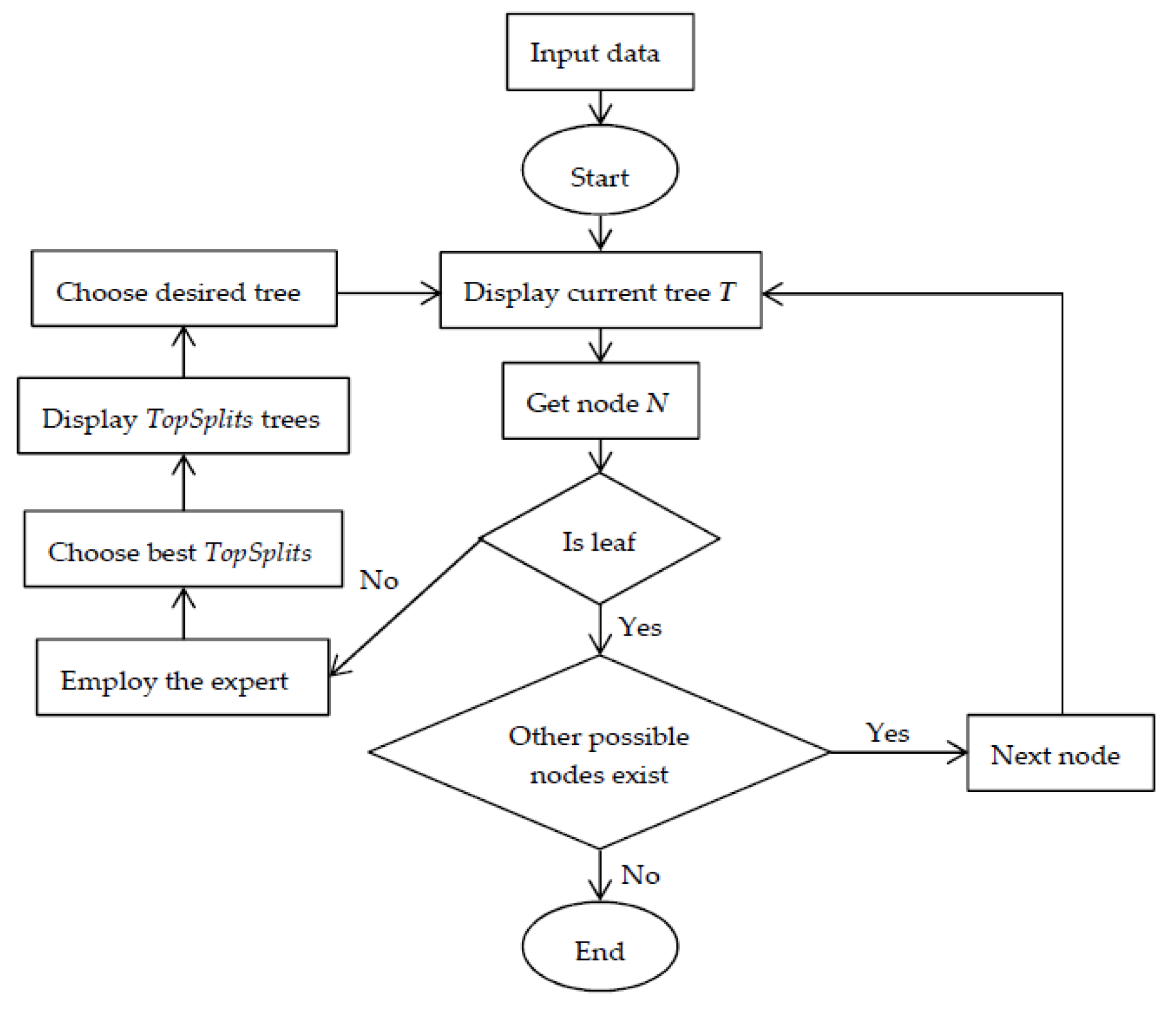
3.2. Algorithm Description
| Algorithm 1: BuildTreeInter algorithm. |
| Input: node (), Yname, Xnames, data, depth, levelPositive, minobs, type, entropypar, cp, ncores, weights, AUCweight, cost, classThreshold, overfit, ambProb, topSplit, varLev, ambClass, ambClassFreq Output: Tree () /1/ node.Count = nrow(data)//number of observations in the node /2/ node.Prob = CalcProb()//assign probabilities to the node /3/ node.Class = ChooseClass()//assign class to the node /4/ splitrule = BestSplitGlobalInter()//calculate statistics of all possible best local splits /5/ isimpr = IfImprovement(splitrule)//check if the possible improvements are greater than the threshold cp /6/ if isimpr is NOT NULL then do /7/ ClassProbLearn()//depending on the input parameters set up learning type /8/ splitrule = InteractiveLearning(splitrule)//start interactive learning (see Algorithm 2) /9/ end /10/ if stop = TRUE then do//check if stopping criteria are met /11/ UpdateProbMatrix()//update global probability matrix /12/ CreateLeaf()//create leaf with various information /13/ return /14/ else do /15/ BuildTreeInter(left )//build recursively tree using left child obtained based on the splitrule /16/ BuildTreeInter(right )//build recursively tree using right child obtained based on the splitrule /17/ end /18/ return |
| Algorithm 2: Interactive learning algorithm. |
| Input: tree (), splitRule, Yname, Xnames, data, depth, levelPositive, minobs, type, entropypar, cp, ncores, weights, AUCweight, cost, classThreshold, overfit, ambProb, topSplit, varLev, ambClass, ambClassFreq Output: Decision regarding splitRule /1/ stopcond = StopCond(splitRule)//check if interactive learning should be performed /2/ if stopcond = TRUE then do//if possible splits are below or above the thresholds, no interaction required /3/ splitrule = Sort(splitRule)//take the best split by sorting in descending order splits according to the gain ratio /4/ return splitrule /5/ end /6/ splitruleInter = Sort(splitRule)//sort in descending order splits according to the gain ratio /7/ if varLev = TRUE then do /8/ splitruleInter = BestSplitAttr(splitruleInter, topSplit)//take the topSplit best splits of each attribute /9/ else do /10/ splitruleInter = BestSplitAll(splitruleInter, topSplit)//take the globally best topSplit splits /11/ end /12/ writeTree()//create output file with the initial tree (current tree structure) /13/ for each splitruleInter do /14/ Tree = Clone()//deep clone of the current tree structure /15/ BuildTree(Tree, left )//build recursively tree using left child obtained based on the splitruleInter /16/ BuildTree(Tree, right )//build recursively tree using right child obtained based on the splitruleInter /17/ if overfit then do /18/ PruneTree(Tree)//prune tree if needed /19/ end /20/ writeTree(Tree)//create output file with the possible tree /21/ end /22/ splitrule = ChooseSplit(splitruleInter)//choose the desired split /23/ return splitrule |
3.3. Software Description
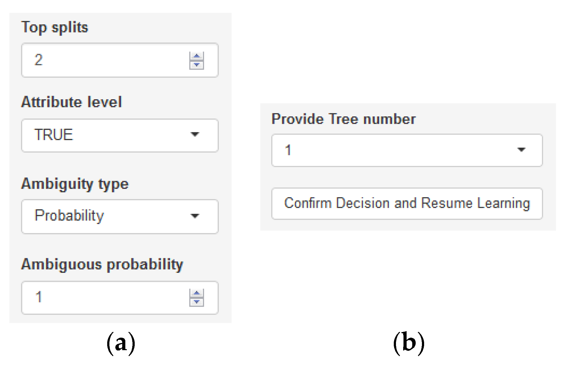
- ambProb: Ambiguity threshold for the difference between the highest class probability and the second-highest class probability per node, below which the expert has to make a decision regarding the future tree structure. This is a logical vector with one element, it works when the ambClass parameter is NULL.
- topSplit: Number of best splits, i.e., final tree structures to be presented. Splits are sorted in descending order according to the gain ratio. It is a numeric vector with one element.
- varLev: Decision indicating whether possible best splits are derived at the attribute level or the split point for each attribute.
- ambClass: Labels of classes for which the expert will make a decision during the learning. This character vector of many elements (from 1 up to the number of classes) should have the same number of elements as the vector passed to the ambClassFreq parameter.
- ambClassFreq: Classes frequencies per node above which the expert will make a decision. This numeric vector of many elements (from 1 up to the number of classes) should have the same number of elements as the vector passed to the ambClass parameter.
4. Extracting Decision Rules
5. Results
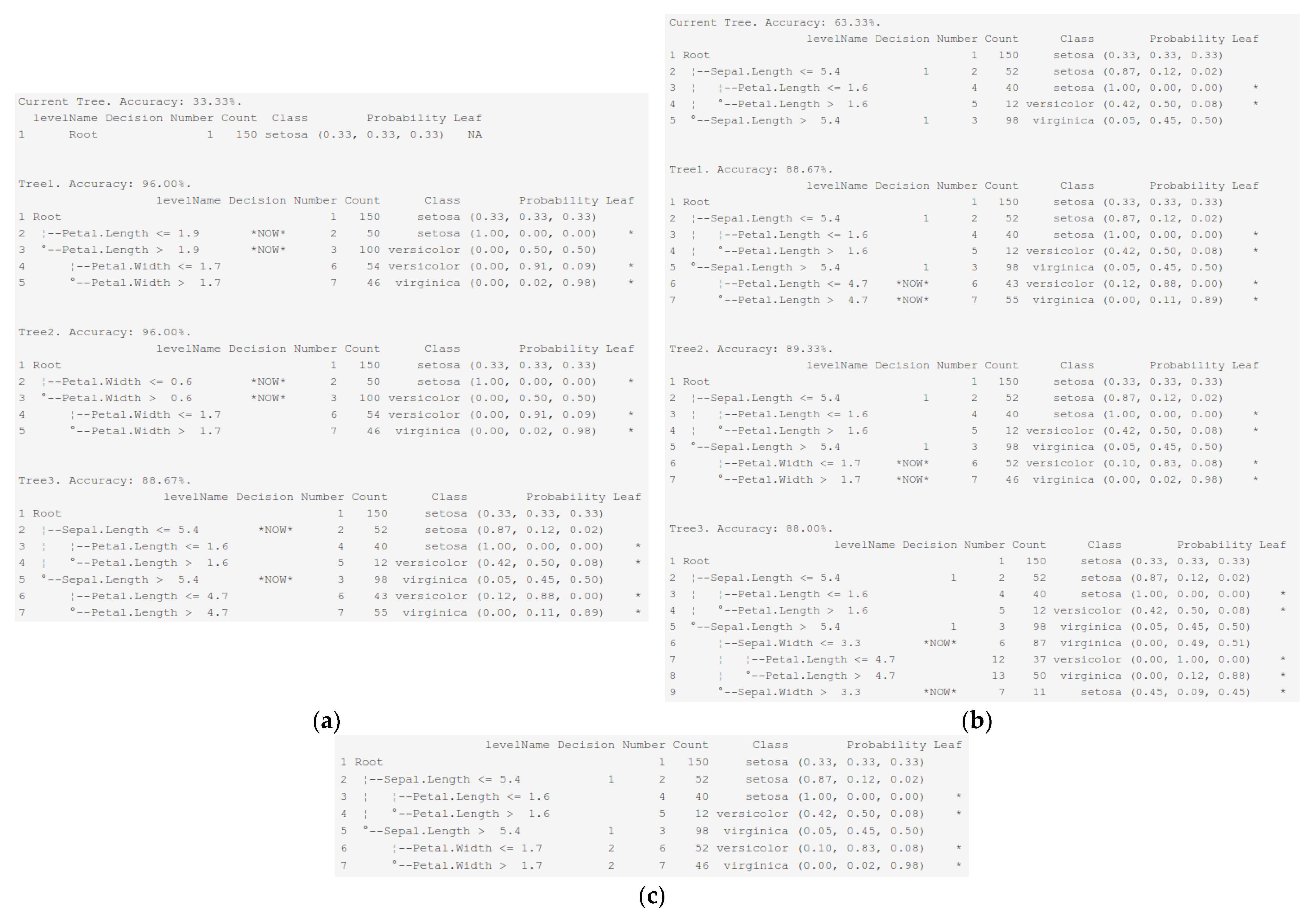
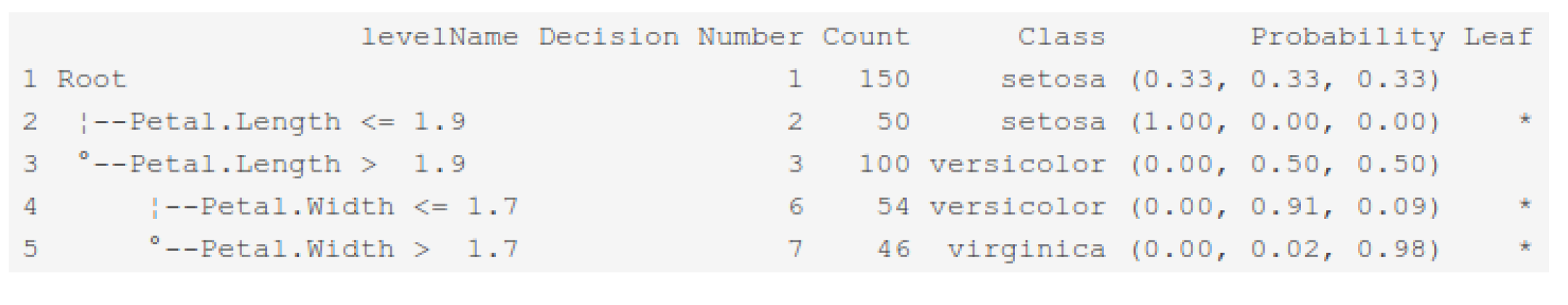
5.1. Interactive Example
5.2. Comparison with Benchmarking Algorithms
- Rpart—package for recursive partitioning for classification, regression and survival trees;
- C50—package that contains an interface to the C5.0 classification trees and rule-based models based on Shannon entropy;
- CTree—conditional inference trees in the party package.
- o
- Three interactive trees trained with ImbTreeEntropy;
- o
- ImbTreeAUC and ImbTreeEntropy trees trained in a fully automated manner (best results after the tuning using a grid search of the possible hyper-parameters) using a 10-fold cross-validation;
- o
- Three benchmarks, i.e., C50, Ctree and Rpart algorithms, that were trained in a fully automated manner (best results after the tuning using grid search of the possible hyper-parameters) using a 10-fold cross-validation.
6. Conclusions
Author Contributions
Funding
Conflicts of Interest
References
- Breiman, L.; Friedman, J.H.; Olshen, R.A.; Stone, C.J. Classification and Regression Trees; Wadsworth Statistics/Probability Series; CRC Press: Boca Raton, FL, USA, 1984. [Google Scholar] [CrossRef] [Green Version]
- Quinlan, J.R. Induction of decision trees. Mach. Learn. 1986, 1, 81–106. [Google Scholar] [CrossRef] [Green Version]
- Kass, G.V. An Exploratory Technique for Investigating Large Quantities of Categorical Data. Appl. Stat. 1980, 29, 119. [Google Scholar] [CrossRef]
- Gajowniczek, K.; Ząbkowski, T. ImbTreeEntropy and ImbTreeAUC: Novel R packages for decision tree learning on the imbalanced datasets. Electronics 2021, 10, 657. [Google Scholar] [CrossRef]
- Ankerst, M.; Ester, M.; Kriegel, H.-P. Towards an effective cooperation of the user and the computer for classification. In KDD’00: Proceedings of the Sixth ACM SIGKDD International Conference on Knowledge Discovery and Data Mining, Boston, MA, USA, 20–23 August 2000; ACM: New York, NY, USA, 2000; pp. 179–188. [Google Scholar] [CrossRef] [Green Version]
- Liu, Y.; Salvendy, G. Design and evaluation of visualization support to facilitate decision trees classification. Int. J. Hum-Comput. Stud. 2007, 65, 95–110. [Google Scholar] [CrossRef]
- Van den Elzen, S.; van Wijk, J.J. BaobabView: Interactive construction and analysis of decision trees. In Proceedings of the 2011 IEEE Conference on Visual Analytics Science and Technology (VAST), Providence, RI, USA, 23–28 October 2011; pp. 151–160. [Google Scholar] [CrossRef] [Green Version]
- Pauwels, S.; Moens, S.; Goethals, B. Interactive and manual construction of classification trees. BENELEARN 2014, 2014, 81. [Google Scholar]
- Poulet, F.; Do, T.-N. Interactive Decision Tree Construction for Interval and Taxonomical Data. In Visual Data Mining. Lecture Notes in Computer Science 2008; Simoff, S.J., Böhlen, M.H., Mazeika, A., Eds.; Springer: Berlin/Heidelberg, Germany, 2008; Volume 4404. [Google Scholar] [CrossRef]
- Tan, P.-N.; Kumar, V.; Srivastava, J. Selecting the right objective measure for association analysis. Inf. Syst. 2004, 29, 293–313. [Google Scholar] [CrossRef]
- Geng, L.; Hamilton, H.J. Interestingness measures for data mining. ACM Comput. Surv. 2006, 38, 9. [Google Scholar] [CrossRef]
- Gajowniczek, K.; Liang, Y.; Friedman, T.; Ząbkowski, T.; Broeck, G.V.D. Semantic and Generalized Entropy Loss Functions for Semi-Supervised Deep Learning. Entropy 2020, 22, 334. [Google Scholar] [CrossRef] [PubMed] [Green Version]
- Gajowniczek, K.; Ząbkowski, T. Generalized Entropy Loss Function in Neural Network: Variable’s Importance and Sensitivity Analysis. In Proceedings of the 21st EANN (Engineering Applications of Neural Networks); Iliadis, L., Angelov, P.P., Jayne, C., Pimenidis, E., Eds.; Springer: Cham, Germany, 2020; pp. 535–545. [Google Scholar] [CrossRef]
- Demsar, J.; Curk, T.; Erjavec, A.; Gorup, C.; Hocevar, T.; Milutinovic, M.; Mozina, M.; Polajnar, M.; Toplak, M.; Staric, A.; et al. Orange: Data Mining Toolbox in Python. J. Mach. Learn. Res. 2013, 14, 2349–2353. [Google Scholar]
- SAS 9.4. Available online: https://documentation.sas.com/?docsetId=emref&docsetTarget=n1gvjknzxid2a2n12f7co56t1vsu.htm&docsetVersion=14.3&locale=en (accessed on 3 March 2021).
- Ankerst, M.; Elsen, C.; Ester, M.; Kriegel, H.-P. Visual classification. In KDD 99: Proceedings of the Fifth ACM SIGKDD International Conference on Knowledge Discovery and Data Mining; ACM: New York, NY, USA, 1999; pp. 392–396. [Google Scholar] [CrossRef]
- Ankerst, M.; Keim, D.A.; Kriegel, H.-P. Circle segments: A technique for visually exploring large multidimensional data sets. In Proceedings of the Visualization, Hot Topic Session, San Francisco, CA, USA, 27 October–1 November 1996. [Google Scholar]
- Liu, Y.; Salvendy, G. Interactive Visual Decision Tree Classification. Human-Computer Interaction. In Interaction Platforms and Techniques; Springer: Berlin/Heidelberg, Germany, 2007; pp. 92–105. [Google Scholar] [CrossRef]
- Han, J.; Cercone, N. Interactive construction of decision trees. In Proceedings of the 5th Pacific-Asia Conference on Knowledge Discovery and Data Mining, Hong Kong, China, 16–18 April 2001; Springer: London, UK, 2001; pp. 575–580. [Google Scholar] [CrossRef]
- Teoh, S.T.; Ma, K.-L. StarClass: Interactive Visual Classification Using Star Coordinates. In Proceedings of the 2003 SIAM International Conference on Data Mining, San Francisco, CA, USA, 1–3 May 2003; pp. 178–185. [Google Scholar] [CrossRef] [Green Version]
- Teoh, S.T.; Ma, K.-L. PaintingClass. In KDD’03: Proceedings of the Ninth ACM SIGKDD International Conference on Knowledge Discovery and Data Mining, Washington, DC, USA, 24–27 August 2003; ACM: New York, NY, USA, 2003; pp. 667–672. [Google Scholar] [CrossRef]
- Liu, D.; Sprague, A.P.; Gray, J.G. PolyCluster: An interactive visualization approach to construct classification rules. In Proceedings of the International Conference on Machine Learning and Applications, Louisville, KY, USA, 16–18 December 2004; pp. 280–287. [Google Scholar] [CrossRef]
- Ware, M.; Frank, E.; Holmes, G.; Hall, M.; Witten, I.H. Interactive machine learning: Letting users build classifiers. Int. J. Hum.-Comput. Stud. 2001, 55, 281–292. [Google Scholar] [CrossRef] [Green Version]
- Poulet, F.; Recherche, E. Cooperation between automatic algorithms, interactive algorithms and visualization tools for visual data mining. In Proceedings of the Visual Data Mining ECML, the 2nd International Workshop on Visual Data Mining, Helsinki, Finland, 19–23 August 2002. [Google Scholar]
- Do, T.-N. Towards Simple, Easy to Understand, and Interactive Decision Tree Algorithm; Technical Report; College of Information Technology, Cantho University: Can Tho, Vietnam, 2007. [Google Scholar]
- Goethals, B.; Moens, S.; Vreeken, J. MIME. In Proceedings of the 17th ACM SIGKDD International Conference on Knowledge Discovery and Data Mining—KDD’11, San Diego, CA, USA, 21–24 August 2011; pp. 757–760. [Google Scholar] [CrossRef]
- Sheeba, T.; Reshmy, K. Prediction of student learning style using modified decision tree algorithm in e-learning system. In Proceedings of the 2018 International Conference on Data Science and Information Technology (DSIT’18), Singapore, 20–22 July 2018; pp. 85–90. [Google Scholar] [CrossRef]
- Nikitin, A.; Kaski, S. Decision Rule Elicitation for Domain Adaptation. In Proceedings of the 26th International Conference on Intelligent User Interfaces (IUI’21), College Station, TX, USA, 14–17 April 2021; pp. 244–248. [Google Scholar] [CrossRef]
- Iris dataset. UCI Machine Learning Repository. Available online: https://archive.ics.uci.edu/ml/index.php (accessed on 10 October 2020).


| Algorithm | Accuracy Train | AUC Train | Accuracy Valid | AUC Valid | Number of Leaves |
|---|---|---|---|---|---|
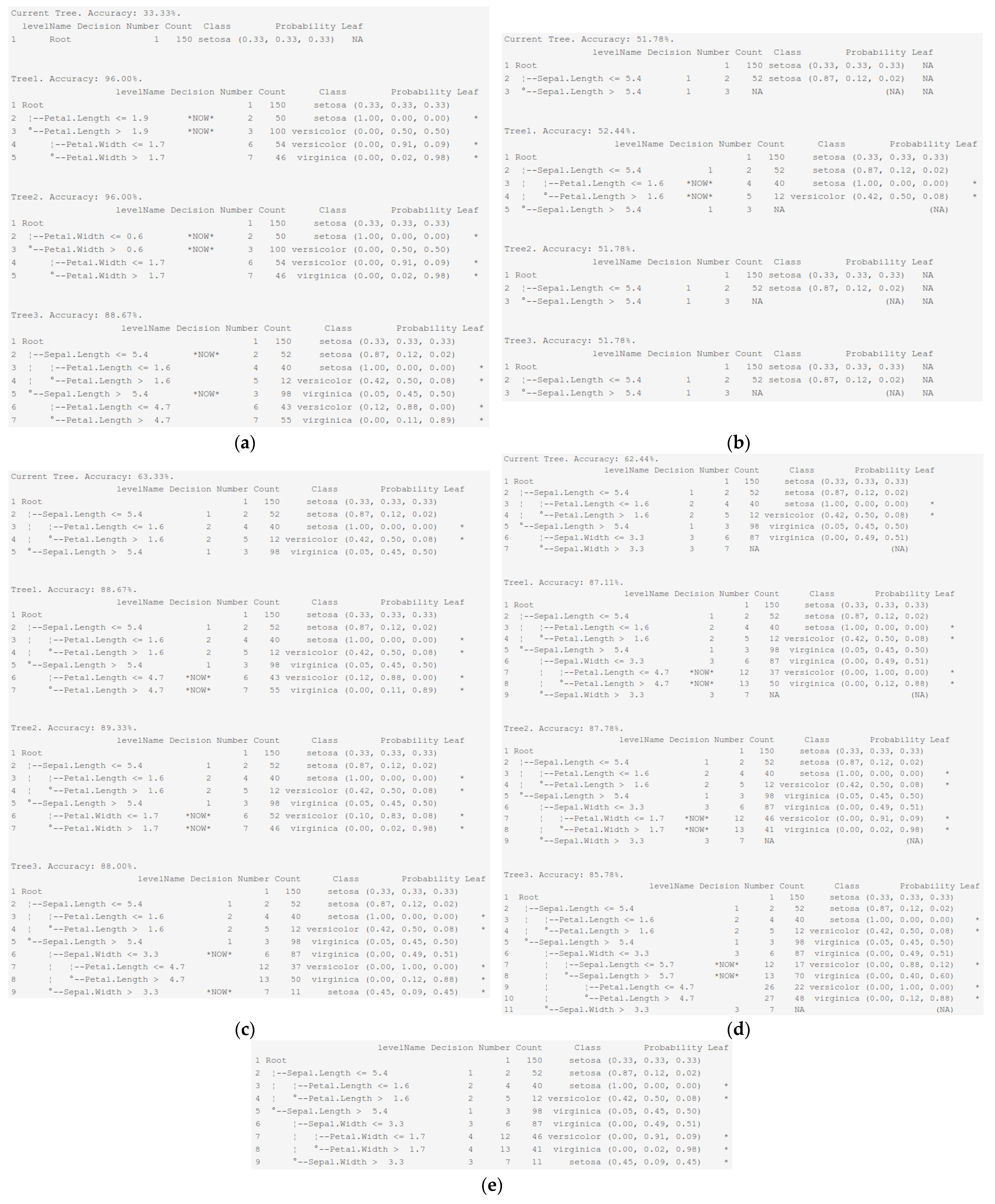
| Interactive ImbTreeEntropy (Figure 3e) | 0.887 | 0.960 | - | - | 5.0 |
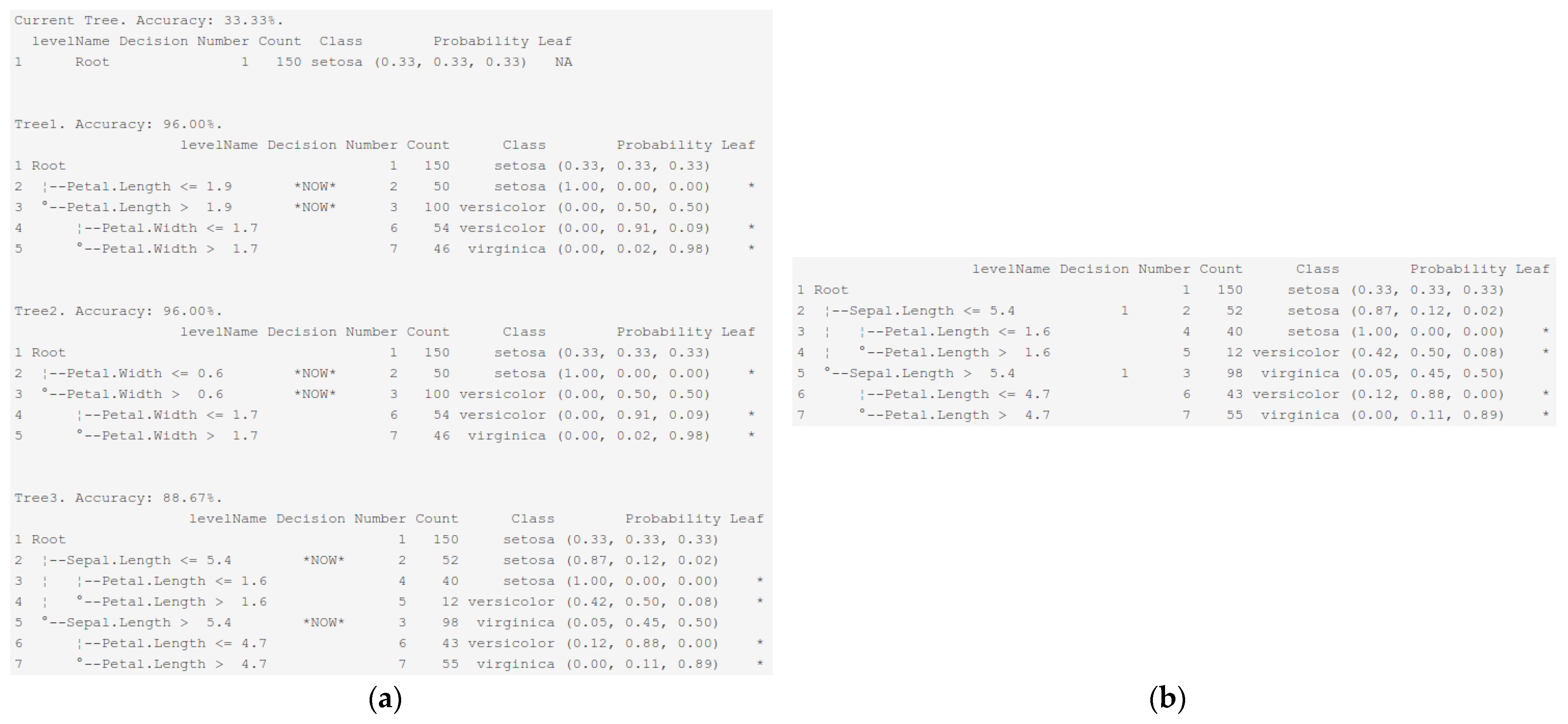
| Interactive ImbTreeEntropy (Figure 5b) | 0.887 | 0.938 | - | - | 5.0 |
| Interactive ImbTreeEntropy (Figure 6c) | 0.893 | 0.938 | - | - | 4.0 |
| ImbTreeAUC | 0.976 (∓0.006) | 0.987 (∓0.006) | 0.960 (∓0.047) | 0.968 (∓0.037) | 3.9 (∓0.316) |
| ImbTreeEntropy | 0.961 (∓0.005) | 0.971 (∓0.004) | 0.947 (∓0.053) | 0.959 (∓0.041) | 3.0 (∓0.000) |
| C50 | 0.976 (∓0.008) | 0.990 (∓0.003) | 0.953 (∓0.055) | 0.971 (∓0.045) | 4.1 (∓0.316) |
| Ctree | 0.976 (∓0.005) | 0.989 (∓0.003) | 0.960 (∓0.034) | 0.971 (∓0.031) | 3.3 (∓0.483) |
| Rpart | 0.973 (∓0.007) | 0.986 (∓0.008) | 0.953 (∓0.032) | 0.961 (∓0.028) | 4.0 (∓0.000) |
Publisher’s Note: MDPI stays neutral with regard to jurisdictional claims in published maps and institutional affiliations. |
© 2021 by the authors. Licensee MDPI, Basel, Switzerland. This article is an open access article distributed under the terms and conditions of the Creative Commons Attribution (CC BY) license (https://creativecommons.org/licenses/by/4.0/).
Share and Cite
Gajowniczek, K.; Ząbkowski, T. Interactive Decision Tree Learning and Decision Rule Extraction Based on the ImbTreeEntropy and ImbTreeAUC Packages. Processes 2021, 9, 1107. https://doi.org/10.3390/pr9071107
Gajowniczek K, Ząbkowski T. Interactive Decision Tree Learning and Decision Rule Extraction Based on the ImbTreeEntropy and ImbTreeAUC Packages. Processes. 2021; 9(7):1107. https://doi.org/10.3390/pr9071107
Chicago/Turabian StyleGajowniczek, Krzysztof, and Tomasz Ząbkowski. 2021. "Interactive Decision Tree Learning and Decision Rule Extraction Based on the ImbTreeEntropy and ImbTreeAUC Packages" Processes 9, no. 7: 1107. https://doi.org/10.3390/pr9071107
APA StyleGajowniczek, K., & Ząbkowski, T. (2021). Interactive Decision Tree Learning and Decision Rule Extraction Based on the ImbTreeEntropy and ImbTreeAUC Packages. Processes, 9(7), 1107. https://doi.org/10.3390/pr9071107