Abstract
Machine learning-based defect identification has emerged as a promising solution to improving the defect accuracy of the aero-engine blade. This solution adopts machine learning classifiers to classify the types of defects. These classifiers are trained to use features collected in ultrasonic echo signals. However, the current studies show the potential number of features, such as statistic values, for identifying defect reaches a number more than that offered by an ultrasonic echo signal. This necessitates multiple acquisitions of echo signal and increases manual effort, and the feature obtained from feature selection is sensitive to the characteristic of the classifier, which further increases the uncertainty of the classifier result. This paper proposes an ensemble learning technique that is only based on few features obtained from an echo signal and still achieves a high accuracy of defect identification as that in traditional machine learning, eliminating the need for multiple acquisitions of the echo signal. To this end, we apply two well-known ensemble learning classifiers and simultaneously compare three widely used machine learning models on defect identification of blades. The result shows that the proposed ensemble learning models outperform machine learning-based models with an equal number of features. In addition, the two-feature-based ensemble learning model reaches an accuracy close to that of multiple statistic features-based machine learning models, where features are obtained from multiple collections of the signal.
1. Introduction
Aero-engine offers a constant power supply to the airplane and plays a key role in the aviation field [1], as shown in Figure 1. The aero-engine is made up of thousands of components, and all of them undergo an adverse working condition, from high temperature or intense radiation to ice-cold, making the components consistently stable and normally operating a challenging task [2]. Thus, it is of great importance to timely and non-destructively monitor the status of components in aero-engine, eliminating the risk that airplanes may encounter in the air.
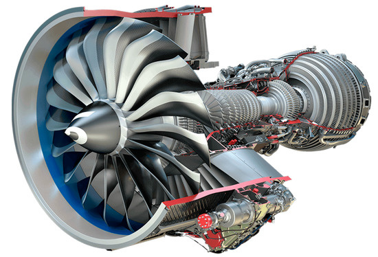
Figure 1.
The cross-section of an aero-engine.
The blade of an aero-engine, the key component in an aero-engine, rotates at high speed and offers forward thrust, suffering a serious environment [3,4]. The status of the blade determines whether the aero-engine could operate or not. Generally, non-destructive testing, especially the ultrasonic pulse-echo testing for convenience and the high-energy wave, is selected for monitoring the status of an aero-engine blade [5,6,7]. The ultrasonic pulse-echo testing on defect identification is promising in terms of the convenience of the device and the penetration power of the high-energy wave. Nevertheless, it is still tough for the inexperienced to differentiate defect from normal and for the skilled to distinguish different defect types [8,9].
The common challenge faced by ultrasonic pulse-echo testing on defect identification is the requirement of carefully operating the flaw detector by a skilled laborer [10,11]. However, this may limit the application of a flaw defector at a specific time; for instance, a skilled laborer is not on duty at midnight. Besides, the similarity of echo waves on different defects, such as the cavity and inclusion, further increases the difficulty in differentiating different types of defects. Moreover, the unevenness of the defect makes the ultrasonic pulse-echo testing based on laborer less practical for defect identification [12].
To address the challenges above, a promising way is to explore the combination of the artificial intelligence method with ultrasonic pulse-echo testing. Machine learning could recognize the hidden pattern behind the pulse-echo signals and classify correctly the test specimen without depending on the experienced laborer. The state-of-the-art machine learning methods on defect identification follow two lines. One is based on abnormal identification, where the key idea is to identify the defect by just utilizing normal pulse-echo signals. They hold the view that the abnormal signal is unpredictable, and any echo signal that does not match normal signals is taken as a defect. We acknowledge its advantage of high accuracy in defect identification; however, it is a coarse-grained method since the type of defect still needs to be ensured when a further step is made, such as improving the quality of a blade or assessing the effects of the defect. The other line is a multi-classifier based on the echo signals of defect. Indeed, the multi-classifier puts aside the skilled laborer and leads to a unique type of defect, while, to achieve the better performance of classification, the feature needed to extract from echo signal reaches up to 12 [13] or 20 [14], which imposes expensive work of extracting features from echo signals onto the laborer.
The features that a lot of work recently requires in its machine learning-based defect identification make collecting plenty of echo signals at a certain position a tough work [15]. Most features are statistic values, such as average frequency, mid-frequency, mean amplitude or the variance of signal amplitude and so on, and each of these statistic features shows different characteristics on different classifiers, which indicates no unique classifier delivers the best results across multiple metrics, thus selecting an algorithm suitable to the specific characteristic becomes a challenge. In addition, feature reduction further exacerbates the identification uncertainty of the classifier since wrongly selected features might reversely decrease the performance. Further, previous studies mostly put their attention on specific learning classifiers and limited types of defects [16]. Thus, exploring an effective model that adopts fewer features as their building basis and does not decrease the performance in defect identification of an aero-engine blade becomes indispensable.
Therefore, the performance of defect identification relies on the number of features and the type of classifier. In this work, we first illustrate the impact of different classifiers as well as the number of features on the accuracy of defect identification. To eliminate the uncertainty of feature selections and classifier characteristics to specific features, a key challenge is how to achieve the performance of the defect identifier under the circumstance of few strongly correlated features exclusively in an ultrasonic echo signal, namely amplitude and frequency sequence, and match that of the identifier under six or twelve features. In this work, we address this challenge by proposing ensemble learning techniques to improve the performance of the defect identifier. The crucial idea is that we can give the final result of defect identification based on the multiple results derived from the corresponding sub-classifier instead of the result that comes from only one classifier, improving the reliability of the ultrasonic test on non-destructive testing. Additionally, we expand the types of defects that each classifier could differentiate, enhancing the application of ultrasonic testing. Each time a pulse-echo signal arrives, each sub-classifier gives a result, normal or the specified defect type, based on the training model learned from the training dataset.
We evaluate the model we proposed with the signal obtained from the normal and defective aero-engine blade. The result shows that different classifiers behave differently based on identical features, and more effective features help to improve the performance of the defect identifier. More importantly, the model we proposed outperforms the state-of-the-art model in identification accuracy under the same feature number. Further, the model we proposed, which is based on two features, has a performance close to that of the state-of-the-art model that depends on six or twelve features.
To conclude, we have three main contributions:
First, we propose a novel ensemble model to identify the concrete defect, namely cavity, crack, slag inclusion and normal state, which exists in an aero-engine blade, enabling us to get a more reliable result.
Second, we analyze the pulse-echo signal of four types of defects existing in an aero-engine blade, expanding the amount of the defect types that the state-of-the-art method could classify.
Third, we validate the effectiveness of our model on defect identification using only two features in pulse-echo signals obtained from normal and defective specimens.
2. Ensemble Learning
Ensemble learning [17] is a learning method that combines base classifiers together to produce a stronger classifier. It predicts the label of the classification or the value of the model based on all the output of the base classifiers, utilizing the complementary information of every base classifier. Compared with the base classifier, ensemble learning output a higher accuracy, and the robustness is better than those of the base classifier. Currently, the most commonly used ensemble learning methods are adaptive boosting and bagging [18]. In this work, we deploy the two widely used ensemble learning methods and explore the effectiveness of ensemble learning in defect identification on an aero-engine blade under a situation that has fewer features.
Adaptive boosting, an ensemble learning model, which is AdaBoost for short, is a stronger classifier that synthesizes multiple base classifiers [19]. AdaBoost enhances the performance by training an additional base classifier based on the instances in the dataset that are misclassified by the former classifier. The procedure of AdaBoost is shown in Figure 2. A base classifier is trained firstly based on an equal weight assigned by the original data sample, and again the weight is updated based on the instances that are wrongly classified. AdaBoost increases the weight of the instances which are wrongly classified in the current iteration to draw more attention in the next iteration. Simultaneously, the weight of the current classifier in the whole strong classifier is calculated depending on the error of the current classifier. Subsequent models are trained and added until the accuracy reaches the threshold, or no further improvement is possible. The final classifier is a combination of the classifier in each iteration with the corresponding weight, in other words, the high weight for the low training error classifier and the low weight for the high training error classifier. In this work, we applied AdaBoost as a boosting learning technique on all commonly used machine learning classifiers to analyze its impact on the accuracy and performance improvement of defect identification of aero-engine blade.
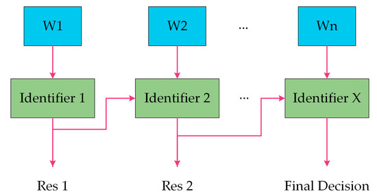
Figure 2.
Block diagrams of the AdaBoost algorithm.
Bagging, or bootstrap aggregation, is another ensemble learning model used in classification or regression fields [20]. Bagging synthesizes the output of multiple classifiers and votes a more appropriate result. The procedure is shown in Figure 3. For bagging, each classifier is trained based on a subset that has an identical distribution with the raw dataset. Bagging decreases the variance of each model and is especially suited for a dataset that has a large variance. Each model in bagging is trained based on a sub-dataset. The sub-dataset is formed by randomly selecting a sample in the raw dataset, iterating times equaling the number of samples in the raw dataset. Thus, the bagging model has a low bias since each model is fully trained under a sub-dataset with different distribution. For each model, the prediction is highly dependent on the data input, and the final output of bagging is an average value or a voted result, a more robust and generalized prediction, of the outputs of multiple classifiers. Therefore, it is most suitable for our purpose, given some classifiers may not be robust to the distribution of datasets and output a result that deviates the normal results.
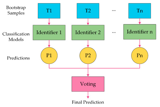
Figure 3.
Block diagrams of the bagging algorithm.
3. Proposed Processing Chain
For the non-destructive testing based on ultrasonic, it is believed that the time-sequence of an ideal echo signal is linearly stationary and Gaussian stochastic, and the noise that this echo signal introduced has a similar time-sequence characteristic. However, the echo signal collected in practice includes various types of noise, such as measuring noise and structure noise. The former is strongly related to the measuring system, and it is a noise not related to the echo signal; thus, it is easy to filter. The latter is a noise strongly coupled with the echo signal, and the large ones will cause useful signals in the echo signal to be drowned out [21,22]. Thus, extracting the effective signal from the echo signal collected is an imperative task.
3.1. Denoising Overview
Currently, multiple denoising algorithms exist, mainly including Fourier transform (FT) and wavelet transform (WT) and empirical mode decomposition (EMD). These algorithms have been validated to effectively remove the noise present in echo signals. FT is suited to deal with noise present in a signal that is linearly stationary, but it is not suited to deal with the details of the signals, leading to distortion while filtering noise out of a signal that is nonlinear and nonstationary. For nonlinear and nonstationary signals, such as ultrasonic echo signals, WT addresses the problem of monitoring the details of signals. Unfortunately, WT introduces the difficulty in selecting a wavelet basis function or decomposition layer [23,24,25,26]. To overcome the difficulty above, the EMD algorithm has been proposed but with drawbacks of mode mixing and end effect. Hence, we choose ensemble empirical mode decomposition (CEEMD) as our denoising algorithm for its effectiveness in solving the mode mixing and end effect.
The procedure of denoising, based on the CEEMD algorithm, mostly decomposes raw signals into a series of intrinsic mode functions (IMF) components. Then, by calculating the coefficients between each IMF to raw signal, it is easy to rank the correlation degree of each IMF to raw signal. Hence, the separation point between signal domain and noise domain can be decided. Finally, the IMF that has a high correlation and a residual signal can be rebuilt as an effective echo signal [27]. However, this procedure has the following limits. It directly removes the IMFs of noise signal away, thus losing the effective details of the noise part. This disadvantage is especially outstanding in ultrasonic echo signal that has a low signal-to-noise ratio, i.e., in signal with large noise.
The second generation wavelet transform (SGWT) algorithm has the advantage of dealing with high-frequency noises. It is a wavelet construction method, which is not based on FT. Utilizing SGWT to deal with the noise part obtained from the CEEMD is of great importance in guaranteeing the integrity of effective signal [28,29].
In this paper, for extracting the effective echo signal, we first calculate the coefficient of IMF (obtained from decomposing raw signal) and raw signal and decide the separation point between signal part and noise part. Then, we extract the details of the noise part utilizing the SGWT method instead of removing them. Finally, we regard rebuilding the signal part as well as the details of the noise part and residual signal as the effective echo signal. Figure 4 details the procedure of obtaining an effective echo signal.
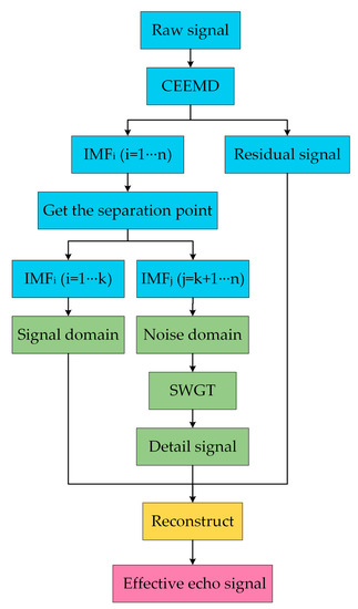
Figure 4.
The details of obtaining an effective echo signal.
3.2. The Details of CEEMD Algorithm
The CEEMD algorithm, a modification of the EMD algorithm, proposed by Yeh is a signal decomposition method for those that are nonlinear and nonstationary time series. As a time–frequency domain analysis method, EMD can decompose the signal into several linear stationary IMFs and a residual signal [30]. As shown in Equation (1):
where is the raw signal with noise; is the IMF; is the number of all IMFs, which contain the ingredients from high-frequency to low-frequency of the raw signal. is the residual signal.
Compared with EMD, the core of the CEEMD method enhancement is that the noise is added to the signal in both positive as well as negative directions in each iteration of signal decomposition, and then the average of all the obtained IMFs will be the final IMFs. The CEEMD procedures can be summarized as follows:
Step 1. Add positive and negative noise signals to the original signal, which can be expressed as:
where is the raw signal; is the added white noise; is the sum of the original data with the positive noise, and is the sum of the original data with the negative noise.
Step 2. EMD Decompose and to two sets of IMFs components and , which contain positive residues and negative residues of added white noise, respectively.
Step 3. Finally, the final IMFs are obtained as follows:
where and contain positive residues and negative residues of added white noise, respectively.
3.3. Determination of Signal Domain and Noise Domain
The IMFs obtained from raw signal decomposing are sorted based on their frequency, and the signal domain is in the IMFs with low frequency, which has a high correlation with the raw signal. Instead, the noise domain is in the IMFs with high frequency, which has a low correlation with the raw signal. Thus, in this paper, we calculate the coefficients of each IMF and raw signal to quantify the separation point between the signal domain and noise domain. The calculation is based on the following:
where is the cross-correlation coefficient between the IMF and the original signal. is the IMF; is the raw signal; is the covariance of ; , and ) are the variance of and , respectively.
By analyzing the correlation of each IMF and raw signal, the separation point between the signal domain and noise domain is determined when the first minimum occurs. Thus, the raw signal could be decomposed into these three parts:
where is the signal domain; is the noise domain; is the separation point of signal domain and the noise domain; is the residual signal.
3.4. The Details of SGWT
SGWT is a time-domain transformation method based on a lifting scheme, getting rid of the dependency of the frequency domain. It is a fast algorithm that is easy to realize and restrains the noise part better in a nonstationary signal [31]. The procedure of applying SGWT on a signal consists of three steps: splitting, predicting and updating, as shown in Figure 5, and the signal rebuilding consists of reverse updating, reverse predicting and combining, as shown in Figure 6.
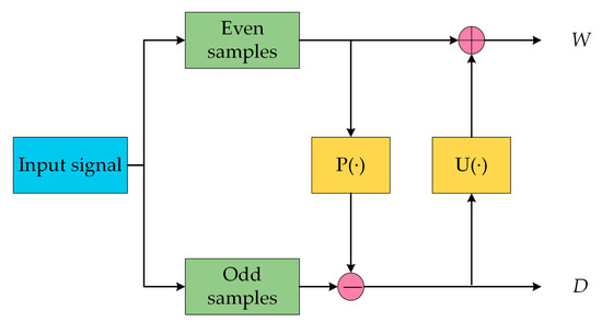
Figure 5.
The second-generation wavelet transformation: a sketch map of decomposition.
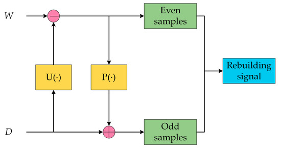
Figure 6.
The second-generation wavelet transformation: a sketch map of reconstruction.
For raw signal with , the even indexed samples are and the odd indexed samples are . As an approximation of the original signal, the even samples are used as a predictor to estimate the odd samples, and the difference between the prediction value and real value is called the wavelet coefficient, which describes the similar degree of two signals, as shown in Equation (6):
where is the prediction operator; is the wavelet coefficient.
To maintain the frequency the characteristic of in the process of transformation, we introduce an update operator and perform updates utilizing to obtain an approximation signal, as shown in Equation (7):
From the perspective of frequency, reflects the high-frequency part of the signal, while reflects the low-frequency part of the signal. We perform the transformation utilizing the Deslauriers–Dubuc (4, 2) wavelet [32], decomposing and rebuilding could be calculated with Equations (8) and (9):
where is the scale level; represents the sampling index number; and are the high-frequency and low-frequency components, respectively. Thus, we can rebuild the effective echo signal for our ensemble learning. The details are written as:
where is effective echo signal, and is signal domain and residual signal obtained, respectively. is the details of noise signal, as shown in the following equation:
where and is the even indexed samples and odd indexed samples of SGWT filtered signal.
Based on the above signal denoising and reconstruction methods, the whole pipeline of our defect identification on the aero-engine blade is shown in Figure 7.
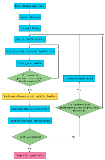
Figure 7.
Block diagram of defect identification.
4. Experiment Setup and Datasets
4.1. Experiment Setup
We are interested in four states of the aero-engine blade, including a normal state that has no defects, cavity or inclusion within the blade, or cracks on the surface of the blade. Based on the defect type we are interested in, we devised the following experiment equipment, as shown in Figure 8. The equipment consists of an ultrasonic signal generator and an oscilloscope, as well as an ultrasonic sensor. We use the ultrasonic generator to actuate the transducer and use the oscilloscope to collect and record the signal sample (here, the sampling frequency of the oscilloscope is 500 MHz). We then convert the analog signal to a digital signal with an 8 bits resolution. Finally, we transmit the digital signal to a computer via a USB port.
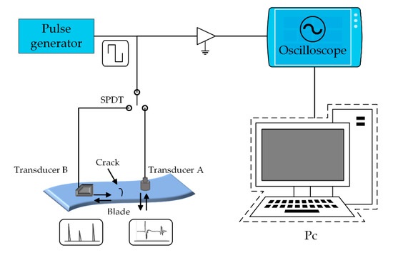
Figure 8.
Diagram of the used experimental setup.
We devise two different transducers to detect different types of defects. For cavity and inclusion, we utilize transducer A with the frequency of 5 MHz and the probe diameter of 14 mm, and we detect the defect in the blade based on the ultrasonic pulse-echo signals received by A. To detect the defect type of crack, we utilize transducer B with the frequency of 5 MHz and an angle probe to generate a signal of Rayleigh wave. The wave travels along the surface of the object. When it arrives at the end of the object or comes across a gap of two different mediums (such as a crack in the surface), the wave reflects and generates an echo signal based on the principle of acoustic impedance, and later this echo signal is received by transducer B. To decrease the variance of detection state due to frequently altering transducer, we place a single-pole double-throw (SPDT) to manage the actuation on the transducer.
4.2. Dataset Collection and Augmentation
The database we use comes from the effective signals, which are filtered from raw echo signals (filtering of raw signals is explained in Section 3). The effective signals comprise four types of echo signal received from the specimen, including cavity, crack, slag inclusion and normal state (See Figure 9). We first choose three specimens that could cover all the defect types. Then, we collect 100 A-scan signals (raw signals) in the interested area on these three specimens. The selection solution of the interested area is as follows. For defect type of slag inclusion and cavity, we define a rectangular grid with an equidistant point (5 mm apart) for the collecting of echo signal. As for the defect type of crack, we define a parallel line 25 mm away from the crack with the spacing of 5 mm for data acquisition. Thirdly, we filter the raw echo signals to obtain the effective signals (for filtering, see Section 3). Given that it is difficult to obtain more specimens to produce the raw signals, instead, we extend the form of effective signals of the four types of echo signals to enhance the dataset. For each type of effective signal, we shift the time-domain signal (including interface signal, bottom signal and defect echo signal) left or right in a fixed expansion randomly 5 times, thus augmenting the dataset size of each type up to 500, and total size of datasets 2500. We shift the signal because the difference of each type of defect varies mainly in size or depth under the surface. Here, 2500 stands for the sum of the five types of signal, three defect types and two normal types. Two types of normal echo signals exist because the transmitting wave is different when testing different defects. For cavity or slag inclusion, it is a longitudinal wave, while it is a Rayleigh wave for the crack.
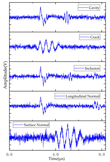
Figure 9.
Echo signals from the specimen of interest.
We extract the feature from the echo signal of ultrasonic testing on the aero-engine blade. As the author [16] has validated, the amplitude and frequency of echo signals play a key role in differentiating whether the object the ultrasonic launch on has defects or not. The experiment they perform demonstrates that the amplitude of the echo signal becomes larger when the size of the defect increases, and the frequency of the echo signal becomes smaller when the defect size increases. Thus, we, as the former research does, select these two features as the main features in our study. Considering that the device we can use in the experiment has not the time–frequency function, we obtain the time–frequency distribution of the signal via the continuous wavelet transform (CWT) on a computer, as shown in Figure 10. Thus, the two-feature vector with amplitude-based sequence and spectrogram-based sequence could be obtained. Then we split the dataset into two parts, where the training dataset is 80 percent, and the other is the testing dataset. The two datasets are used for training and testing the classifier. We follow the rules that the testing process comes strictly after the training process.
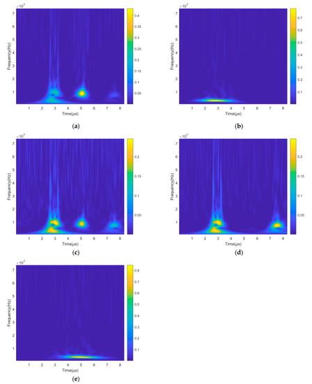
Figure 10.
The feature from the echo signal of ultrasonic testing. (a) Time–frequency distribution of cavity state; (b) Time–frequency distribution of crack state; (c) Time–frequency distribution of inclusion state; (d) Time–frequency distribution of longitudinal normal state; (e) Time–frequency distribution of surface normal state.
4.3. Evaluation Metrics
In this section, we detail the metrics for our experiment evaluation. As two classification cases, we choose accuracy and precision as well as F1 score as our evaluation criterion, and we do not consider what type the instance wrongly classified has been assigned. The accuracy demonstrates the ability of the classifier on the defect detected among all the true defect samples, and the precision illustrates the true parts among all the classified types. The F1 score is a comprehensive evaluation index, which balances the accuracy and precision. Precision and accuracy reflect the performance of the classifier from different aspects, while the F1 score reflects the performance of the classifier on the whole.
where is the accuracy of the classifier; is the precision of the classifier on identifying. is the true positive; is the false negative; is the false positive.
4.4. Baseline Approaches
Here, we include three machine learning methods for our comparison basis, which are multiple layer perceptron (MLP), Logic Regression (LR), and support vector machine (SVM). The three machine learning methods have been observed to perform better when the input features are over a dozen [13,14], eliminating the probability of bad performance due to algorithm selection. The baseline models and ensemble learning models are all trained and tested on the same datasets.
5. Evaluation
In the following, we compare the defect identification performance of ensemble learning with baselines. We first illustrate the defect identification result of different classifiers for the same feature number and again compare the impact of the number of features on the performance. Then we detail the result of each method based on two features.
Clearly, we can see in Figure 11 different classifiers perform distinctively on the defect identification with the feature vector, including two features (For more details, refer to Table 1 and Table 2). The difference derives from the intrinsic characteristic of the classifier. On the one hand, some classifiers have a better detection ability on the nonlinear characteristic of the input, such as SVM, and some have a better detection ability on the linear input, for instance, the LR. On the other hand, the relationship among features also affects the performance of each defect identifier. For the first case, the two features we selected have no linear relationship; thus, LR performs worse (only 0.79) compared to SVM. Additionally, SVM fits the relationship better due to the strongly expression ability of the kernel function. Here, the multiple layer perceptron (or the neural network) on defect identification behaves badly as the feature number in the feature vector is too small.
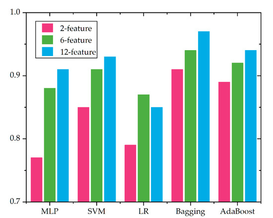
Figure 11.
The average accuracy of different algorithms on the identification of different defect types of aero-engine blades.

Table 1.
The average accuracy of different algorithms on the identification of different defect types of aero-engine blades.
Table 2.
The accuracy of different algorithm on the identification of different defect types of aero-engine blade.
To fully compare the effect of the feature number on the defect identification performance, we extend our feature number to six [33] and twelve [13]. Considering the type number and for brevity, we calculate the average accuracy of each algorithm on the type identification of the blade. The result is shown in Table 1. Overall, we can see that with the number of features decreasing, the accuracy declines distinctly (note that the value in the figure illustrates the average value, including the type of normal blade), and the details of each algorithm are given in Table 2. However, it is interesting that although the feature number declines, the accuracy of ensemble learning decreases slightly. To some extent, the accuracy of the 2-feature based ensemble learning algorithm is numerically close to that of the 6-feature based or 12-feature based algorithm, which demonstrates the feasibility and practicability of an ensemble learning algorithm even in few feature environments.
Table 3 shows the F1 score of the different algorithms on the identification for different defect types of aero-engine blade. At a high level, we can see the F1 score of the bagging and boosting outperforms the other machine learning algorithms. Moreover, bagging performs particularly better for each type of defect and more than 15% higher than that of other algorithms. Note that all the algorithms behave badly on differentiating cavity and inclusion defects. This is because the difference between these two types of echo signals is especially small and differentiating them necessitates the aid of other features, which could not be obtained via the echo signal, such as an elemental analyzer for analyzing. Note that our attention focuses on feature reduction while still maintaining the performance of defect identification.
Table 3.
The F1 score of different algorithms on the identification of different defect types of an aero-engine blade.
As Table 3 illustrates, the F1 score increasing of ensemble learning algorithms derive from the increase in recall value. Even though the F1 score is not very good (0.8 or so) on these three defects, the recall value reaches up to 0.9, which indicates the defect type could be identified most of the time. On the other hand, the recall value of the base methods is all below 0.9, and some even have smaller values (such as 0.65); thus, the base methods regard about 30% of samples as normal, leaving uncertainty on the aero-engine blade in practice.
6. Related Works
The defect identification of an aero-engine blade mainly consists of three parts, including manual inspection, traditional inspection and machine learning-based defect inspection. For manual inspection, it requires a skilled inspector to judge whether the blade has a defect or not, decreasing the correctness of the judgement. It only applies in some domains that do not have measurements available.
Traditional defect identification of aero-engine blade is on the basis of defect inspection on metal, where the threshold is determined before performing a defect identification. The threshold could be determined by the experienced specialist, and any person who lacks special training may wrongly identify defects based on the measurement result and threshold. However, this kind of defect identification lacks reliability since the measurement result may vary in different conditions or the threshold differs with a different batch of blades.
Machine learning is widely used in defect identification [15]. Similarly, this algorithm can be utilized in the defect identification of aero-engine blade. The primary issue of machine learning-based defect identification is feature selection. Feature selection is a critical step and consists of expensive work. One can decrease to a small number of features at the sacrifice of accuracy, while a large number of features increase manual cost and redundancy in features, which in turn decreases the accuracy. Currently, the number of features reaches up to ten or more [13,14], imposing a burden on manual work. In contrast, our work aims at pursuing an accuracy with a small number of features and achieving an accuracy as high as that with a large number of features in machine learning. We select ensemble learning as the main algorithm in machine learning, which depends on the result of multiple simple classifiers or weak classifiers, and only two features are chosen, eliminating the cost of manual effort. We do not consider deep learning algorithm in defect identification, even though it automatically extracts the feature from echo signal.
7. Conclusions
In this paper, we propose utilizing ensemble learning technique on defect identification of an aero-engine blade. Ensemble learning-based defect identifiers utilize features extracted only from an ultrasonic signal, which leaves out the statistic features obtained from multiple acquisitions of echo signals, thus simultaneously decreasing the expensive manual cost. It integrates multiple sub-classifiers and accurately identifies different defect types of the blade, eliminating the uncertainty in feature selections and the intrinsic characteristic of a classifier to a specific feature. With the same number of features, ensemble learning-based defect identifiers outperform the state-of-the-art classifier on defect identification of aero-engine blade. Morevoer, using a dataset including only two features in blade defect identification, the performance of ensemble learning closely approaches that of the existing algorithms based on more than six features or even twelve features.
Author Contributions
Conceptualization, Y.J. and Z.L.; methodology, Y.J., Z.L. and B.Z.; investigation, Y.J., J.Z. and Z.L.; data curation, J.Z., Z.L. and B.Z.; writing—review and editing, Y.J., Z.L., J.Z., B.X. and B.Z.; supervision, B.X. and B.Z.; project administration, B.Z. and Z.L.; funding acquisition, B.X. and Z.L. All authors have read and agreed to the published version of the manuscript.
Funding
This research was funded by the intelligent online diagnosis system of railway color light signal machine filament relay based on big data, grant number 18YFCZZC00320, the National Natural Science Foundation of China, grant number 62075162, and the Natural Science Foundation of Tianjin, grant number 18JCYBJC17100.
Institutional Review Board Statement
Not applicable.
Informed Consent Statement
Not applicable.
Data Availability Statement
Not applicable.
Acknowledgments
The authors acknowledge the financial support from the intelligent online diagnosis system of railway color light signal machine filament relay based on big data (Grant No. 18YFCZZC00320), the National Natural Science Foundation of China (Grant No. 62075162) and the Natural Science Foundation of Tianjin (Grant No. 18JCYBJC17100).
Conflicts of Interest
The authors declare no conflict of interest.
References
- Zhu, R.; Liang, Q.; Zhan, H. Analysis of aero-engine performance and selection based on fuzzy comprehensive evaluation. Procedia Eng. 2017, 174, 1202–1207. [Google Scholar] [CrossRef]
- Wang, C.; Lu, N.; Cheng, Y.; Jiang, B. A data-driven aero-engine degradation prognostic strategy. IEEE Trans. Cybern. 2019, 99, 1–11. [Google Scholar] [CrossRef]
- Zhang, K.; Liu, Y.; Liu, S.; Zhang, X.; Qian, B.; Zhang, C.; Tu, S. Coordinated bilateral ultrasonic surface rolling process on aero-engine blades. Int. J. Adv. Manuf. Technol. 2019, 105, 4415–4428. [Google Scholar] [CrossRef]
- Yao, S.; Cao, X.; Liu, S.; Gong, C.; Zhang, K.; Zhang, C.; Zhang, X. Two-sided ultrasonic surface rolling process of aeroengine blades based on on-machine noncontact measurement. Front. Mech. Eng. 2020, 15, 240–255. [Google Scholar] [CrossRef]
- Gao, C.; Meeker, W.Q.; Mayton, D. Detecting cracks in aircraft engine fan blades using vibrothermography nondestructive evaluation. Reliab. Eng. Syst. Saf. 2014, 131, 229–235. [Google Scholar] [CrossRef]
- Li, W.; Zhou, Z.; Li, Y. Inspection of butt welds for complex surface parts using ultrasonic phased array. Ultrasonics 2019, 96, 75–82. [Google Scholar] [CrossRef]
- Li, J.J.; Yan, C.F.; Rui, Z.Y.; Zhang, L.D.; Wang, Y.T. A Quantitative Evaluation Method of Aero-engine Blade Defects Based on Ultrasonic C-Scan. In Proceedings of the 2020 IEEE Far East NDT New Technology & Application Forum (FENDT), Nanjing, China, 20–22 November 2020; pp. 91–95. [Google Scholar] [CrossRef]
- Fortunato, J.; Anand, C.; Braga, D.F.; Groves, R.M.; Moreira, P.M.G.P.; Infante, V. Friction stir weld-bonding defect inspection using phased array ultrasonic testing. Int. J. Adv. Manuf. Technol. 2017, 93, 3125–3134. [Google Scholar] [CrossRef]
- Droubi, M.G.; Faisal, N.H.; Orr, F.; Steel, J.A.; El-Shaib, M. Acoustic emission method for defect detection and identification in carbon steel welded joints. J. Constr. Steel Res. 2017, 134, 28–37. [Google Scholar] [CrossRef]
- Hauser, M.; Amamcharla, J.K. Development of a method to characterize high-protein dairy powders using an ultrasonic flaw detector. J. Dairy Sci. 2016, 99, 1056–1064. [Google Scholar] [CrossRef] [PubMed]
- Mogilner, L.Y.; Smorodinskii, Y.G. Ultrasonic flaw detection: Adjustment and calibration of equipment using samples with cylindrical drilling. Russ. J. Nondestruct. Test. 2018, 54, 630–637. [Google Scholar] [CrossRef]
- Ding, H.; Qian, Q.; Li, X.; Wang, Z.; Li, M. Casting Blanks Cleanliness Evaluation Based on Ultrasonic Microscopy and Morphological Filtering. Metals 2020, 10, 796. [Google Scholar] [CrossRef]
- Sambath, S.; Nagaraj, P.; Selvakumar, N. Automatic defect classification in ultrasonic NDT using artificial intelligence. J. Nondestruct. Eval. 2011, 30, 20–28. [Google Scholar] [CrossRef]
- Cruz, F.C.; Simas Filho, E.F.; Albuquerque, M.C.S.; Silva, I.C.; Farias, C.T.T.; Gouvêa, L.L. Efficient feature selection for neural network based detection of flaws in steel welded joints using ultrasound testing. Ultrasonics 2017, 73, 1–8. [Google Scholar] [CrossRef]
- Alsaeedi, A.; Khan, M.Z. Software defect prediction using supervised machine learning and ensemble techniques: A comparative study. J. Softw. Eng. Appl. 2019, 12, 85–100. [Google Scholar] [CrossRef]
- Xiao, H.; Chen, D.; Xu, J.; Guo, S. Defects identification using the improved ultrasonic measurement model and support vector machines. NDT E Int. 2020, 111, 102223. [Google Scholar] [CrossRef]
- Freund, Y.; Schapire, R.E. A decision-theoretic generalization of on-line learning and an application to boosting. J. Comput. Syst. Sci. 1997, 55, 119–139. [Google Scholar] [CrossRef]
- Sayadi, H.; Patel, N.; PD, S.M.; Sasan, A.; Rafatirad, S.; Homayoun, H. Ensemble learning for effective run-time hardware-based malware detection: A comprehensive analysis and classification. In Proceedings of the 2018 55th ACM/ESDA/IEEE Design Automation Conference (DAC), San Francisco, CA, USA, 24–28 June 2018; pp. 1–6. [Google Scholar] [CrossRef]
- Liang, S.; Wang, L.; Zhang, L.; Wu, Y. Research on recognition of nine kinds of fine gestures based on adaptive AdaBoost algorithm and multi-feature combination. IEEE Access 2018, 7, 3235–3246. [Google Scholar] [CrossRef]
- Hothorn, T.; Lausen, B. Double-bagging: Combining classifiers by bootstrap aggregation. Pattern Recognit. 2003, 36, 1303–1309. [Google Scholar] [CrossRef]
- Thong-un, N.; Hirata, S.; Orino, Y.; Kurosawa, M.K. A linearization-based method of simultaneous position and velocity measurement using ultrasonic waves. Sens. Actuators A Phys. 2015, 233, 480–499. [Google Scholar] [CrossRef]
- Wu, B.; Huang, Y.; Krishnaswamy, S. A Bayesian approach for sparse flaw detection from noisy signals for ultrasonic NDT. NDT E Int. 2017, 85, 76–85. [Google Scholar] [CrossRef]
- Zhai, M.Y. Seismic data denoising based on the fractional Fourier transformation. J. Appl. Geophys. 2014, 109, 62–70. [Google Scholar] [CrossRef]
- Zhao, R.M.; Cui, H.M. Improved threshold denoising method based on wavelet transform. In Proceedings of the 2015 7th International Conference on Modelling, Identification and Control (ICMIC), Sousse, Tunisia, 8–20 December 2015; pp. 1–4. [Google Scholar] [CrossRef]
- Tian, P.; Cao, X.; Liang, J.; Zhang, L.; Yi, N.; Wang, L.; Cheng, X. Improved empirical mode decomposition based denoising method for lidar signals. Opt. Commun. 2014, 325, 54–59. [Google Scholar] [CrossRef]
- Mohammadi, M.H.D. Improved Denoising Method for Ultrasonic Echo with Mother Wavelet Optimization and Best-Basis Selection. Int. J. Electr. Comput. Eng. 2016, 6, 2742. [Google Scholar] [CrossRef][Green Version]
- Torres, M.E.; Colominas, M.A.; Schlotthauer, G.; Flandrin, P. A complete ensemble empirical mode decomposition with adaptive noise. In Proceedings of the 2011 IEEE International Conference on Acoustics, Speech and Signal Processing (ICASSP), Prague, Czech Republic, 22–27 May 2011; pp. 4144–4147. [Google Scholar] [CrossRef]
- Erçelebi, E. Second generation wavelet transform-based pitch period estimation and voiced/unvoiced decision for speech signals. Appl. Acoust. 2003, 64, 25–41. [Google Scholar] [CrossRef]
- Zheng, H.; Dang, C.; Gu, S.; Peng, D.; Chen, K. A quantified self-adaptive filtering method: Effective IMFs selection based on CEEMD. Meas. Sci. Technol. 2018, 29, 085701. [Google Scholar] [CrossRef]
- Yeh, J.R.; Shieh, J.S.; Huang, N.E. Complementary ensemble empirical mode decomposition: A novel noise enhanced data analysis method. Adv. Adapt. Data Anal. 2010, 2, 135–156. [Google Scholar] [CrossRef]
- Sweldens, W. The lifting scheme: A construction of second generation wavelets. SIAM J. Math. Anal. 1998, 29, 511–546. [Google Scholar] [CrossRef]
- Calderbank, A.R.; Daubechies, I.; Sweldens, W.; Yeo, B.L. Lossless image compression using integer to integer wavelet transforms. In Proceedings of the International Conference on Image Processing, Santa Barbara, CA, USA, 26–29 October 1997; Volume 1, pp. 596–599. [Google Scholar] [CrossRef]
- Chiou, C.P.; Schmerr, L.W.; Thompson, R.B. Review of Progress in Quantitative Nondestructive Evaluation; Springer: Boston, MA, USA, 1993; p. 789. [Google Scholar]


Publisher’s Note: MDPI stays neutral with regard to jurisdictional claims in published maps and institutional affiliations. |
© 2021 by the authors. Licensee MDPI, Basel, Switzerland. This article is an open access article distributed under the terms and conditions of the Creative Commons Attribution (CC BY) license (https://creativecommons.org/licenses/by/4.0/).