Article

Comparison of Different Numerical Interface Capturing Methods for the Simulation of Faraday Waves

1
Facultad de Ciencias de la Ingeniería, Instituto de Materiales y Procesos Termomecánicos, Universidad Austral de Chile, Valdivia 5090000, Chile
2
Departamento de Mecánica, Universidad Simón Bolívar, Caracas 1080, Venezuela
3
INPT, UPS, IMFT, Universite de Toulouse, 31400 Toulouse, France
*
Author to whom correspondence should be addressed.
Processes 2021, 9(6), 948; https://doi.org/10.3390/pr9060948
Submission received: 29 April 2021 / Accepted: 21 May 2021 / Published: 27 May 2021
(This article belongs to the Special Issue Advancement in Computational Fluid Mechanics and Optimization Methods)

Abstract

:
Faraday instability is a classic problem that occurs due to the relative displacement of the interface that separates two immiscible fluids placed in a closed container under oscillating acceleration parallel to gravity. The interface deformation and the induced flow patterns of this two-phase flow are very complex and numerical simulations could allow a deeper understanding of the dynamics of these systems. Some tests have been performed to establish a reference solution, but further validation is needed in order to ensure the validity of these solutions. In this work, we compare some numerical solutions for the linear and nonlinear regimes using the phase field scheme with predictions obtained using different numerical schemes such as Front Tracking, Volume of Fluid, and Element-based Finite Volume Method. The results show that, in both linear and nonlinear regimes, some important differences in the prediction of the interface dynamics between the methods are observed, and the need to provide a reference numerical solution for future benchmarks is highlighted.

1. Introduction

Instabilities in mechanical systems are present in many areas of engineering processes [1]. In general, the response of different variables of a mechanical system can be especially sensitive to changes in one or several parameters [2]. For example, in the well-known Melde’s experiments [3] in which a horizontal string is subjected to a tension at one end and made to vibrate at the other end, the formation of standing waves is possible for specific values of the excitation frequency that depends on geometrical and dynamic variables such as the length and tension of the string. In this case, the parameter controlling the wave pattern is the excitation frequency. Determining the value of the parameter range or the phase space of the parameter set, where the system is stable or not, is crucial in many applications.
The dynamics of some fundamental and industrial applications of mechanical systems involving fluids is based on the same principles. Applications include spray formation [4], liquid atomization [5], and the creation of liquid-based templates to generate patterns to print micro-structures [6]. In particular, many natural phenomena and industrial processes originate due to the effects caused by the acceleration of a container or vessel containing two fluids (both liquids or a liquid and a gas) separated by an interface. The occurrence of an instability at the interface is taken advantage of, which may result in the appearance of standing wave patterns or the detachment of small droplets of the denser fluid. This instability will be of a different nature depending on how the acceleration is applied [7]. Indeed, depending on whether the applied acceleration is constant, impulsive, or harmonic, instabilities such as Rayleigh–Taylor [8], Richtmyer–Meshkov [9], or Faraday [10] occur, respectively. Often, the solutions of the governing equations are very sensitive to the parameters that trigger the instability and describing their phase space can be a very difficult task [11]. In addition, analytic solutions for the governing equations are often not available and numerical methods have to be employed to find approximate solutions. Special care must be taken when considering different numerical approaches to ensure that the solutions are independent of the discretization scheme chosen to represent the governing equations.
In this work, we are interested in the numerical simulation of Faraday instability [10]. This instability is produced by the relative displacement of the interface separating two non-miscible fluids placed in a closed container, subjected to an oscillating acceleration parallel to gravity. If both fluids and the container are at rest, the interface that separates both fluids is flat. Faraday [10] found that, for a given value of the frequency of the oscillating acceleration, when values of the amplitude of the oscillating acceleration, a f , are below a critical value, a c , no appreciable motion of the interface is observed, and any perturbation of the interface is dissipated. Otherwise, if a f is greater than a c , the interface becomes unstable showing complex behavior. Under certain conditions, for the threshold value a c , the interface separating both fluids shows a regular standing waves pattern. Faraday [10] observed that, when a f value corresponds to the threshold value a c , the frequency of the standing waves was half the frequency of the acceleration of the container while Matthiessen [12] reported that the frequency was equal to that of the container. The value of a c is a function of the dimensions of the container, the physical properties of fluids, and the oscillating frequency.
Several efforts have been made in the past to determine the values of critical parameters for the Faraday instability and to analyze the interface behavior for values of a f greater than a c . The study of Faraday instability has been approached by considering two different regimes, linear and nonlinear. In the linear regime, the terms of the equations of motion involving products between velocity components, or with its derivatives, are neglected as Kumar [2] does. A variation of this approach is called weakly nonlinear and consists of expanding the nonlinear terms and neglecting the fourth- and higher-order terms [12]. Consequently, in the linear regime, the oscillation amplitudes of the interface must be relatively small compared to the wave length, so the convective term in the equations of motion can be neglected in the governing equations.
The Faraday instability has been analyzed by many authors. Kumar and Tuckerman [2] determine the critical values of the oscillating acceleration magnitude as a function of the wavenumber for a two-dimensional system consisting of a rectangular container with two ideal fluids separated by a planar interface using a Floquet analysis. They found that, for the threshold value, standing waves could be harmonic or sub-harmonic with frequencies that are equal to or half the oscillating acceleration, respectively.
Subsequently, Wright et al. [7] compare, for non-viscous fluids, the solutions from a boundary-integral method with the vortex-sheet method. For small interface deformations, the predictions of both methods are very similar. They found that plumes, droplet formation, and ejection could appear for moderate values of the Atwood number.
The Faraday instability with viscous fluids is studied by Kumar [13] who presents a linear analysis. He found that, for the same value of frequency and amplitude of the oscillating acceleration, it is possible to have both harmonic and sub-harmonics’ standing waves patterns. Later, Périnet et al. [14] use a finite-difference projection method coupled with a front-tracking method to track the interface. They perform analyses in two and three dimensions and their results for the threshold values of the oscillating acceleration amplitude are in good agreement with the Floquet analysis of Kumar and Tuckerman [2]. In order to validate the numerical results of Périnet et al. [14] with a different numerical method, Takagi and Matsumoto [15] use a numerical scheme based on the phase-field method. They perform an analysis for both linear and nonlinear regimes. Their results for the magnitude of the critical acceleration in the linear regimes are in good agreement with those of Périnet et al. [14], but, in the nonlinear regime, the comparison of the interface dynamics in their test case, taken from Wright et al. [7], is only qualitative due to differences between properties of fluids (densities), the size of the physical domain, and the consideration of viscous effects. Takagi and Matsumoto [15] show that the trends of the interface dynamics is similar in both methods and conclude that their model is able to provide accurate numerical results of the Faraday instability. Other different nonlinear cases are tested and show good agreement with experimental results of Jiang et al. [16], in particular, concerning the occurrence of the period tripling of standing waves. Takagi and Matsumoto perform another study [17] of the same mechanical system considering a two-frequency forcing, but they use a different numerical scheme, the particle-level method, to model the interface dynamics. Accurate modeling of the forces due to interfacial tension is very important to adequately describe the interface dynamics. Different methodologies are used to represent the effect of surface tension, depending on how it is represented. The region that separates fluids can be represented, in grid-based methods, as a diffuse or a sharp interface. The natural choice for representing interfacial forces, based on the definition of the forces themselves, is to express them as tangential forces to the interface. This method then requires defining the interface using adaptive meshes so that the interface coincides with a surface (line in 2D flows) of the grid, or, in fixed meshes, by introducing a set of markers that represent the interface and move with the flow. Methods using adaptive moving meshes allow interfacial conditions on the tangential and normal stresses of the surface to be imposed in a natural way, but have limitations in their application when the interface deforms considerably [18]. On the other hand, there are methods that use markers that are carried by the flow and allow for tracking the interface. These methods allow for considering large curvatures but have the disadvantage that can lead to interfaces that deform at spatial scales that cannot be represented in the grid [19]. Among the methods belonging to this family is Front Tracking [20].
On the other hand, another family of methods uses diffuse interfaces for which the term representing the interfacial forces is expressed as a volumetric distribution of forces. In this case, this originally local force (appearing only at the interface) is distributed over a small set of cells. For this purpose, the function representing an interface concentrated in a region of space is approximated by a Heaviside function that extends the interface in a direction perpendicular to itself, an ad-hoc distance (usually the width of a domain cell). The interfacial forces are then calculated from an integration over the entire fluid domain. Volume-of-fluid type methods use this approach [19]. Popinet [21] presents an excellent review of methodologies to calculate these interfacial forces.
To consider Takagi and Matsumoto [15] results as reference solutions for the 2D Faraday instability, a few points must be well established. First, comparisons in linear regime must go beyond checking in a number of cases the computed values for the critical acceleration. The dynamics of the interface must be analyzed to be sure that the actual motion is accurately represented. In addition, the comparison with the nonlinear case must also be verified quantitatively, since Takagi and Matsumoto [15] only compare qualitative trends of the interface movement at the midpoint of the container and the formation of plumes. In their simulation, Takagi and Matsumoto [15] use fluid density values different than those of Wright et al. [7] due to limitations in their implementation of the phase-field scheme to consider high Atwood numbers. In addition, the results of Wright et al. [7] were obtained in a semi-infinite domain; consequently, the influence of fluid confinement on the interface dynamics could be important.
In this work, different numerical schemes are considered for the simulation of the two-dimensional Faraday instability. We use three different codes, two in-house codes based on Front-tracking (sharp interface representation) and Volume of Fluid (diffuse interface representation) methods, respectively, to shift the interface, and the commercial software ANSYS-CFX (Element-based Finite Volume Method). We consider cases in the linear and nonlinear regimes in the same manner as Takagi and Matsumoto [15]. Comparison of the threshold accelerations and interface dynamics for the linear harmonic and sub-harmonic cases and a nonlinear case resulting in the formation of a plume have been considered.
This paper is organized as follows: first, we describe the physical domain, the mathematical framework, and the particular features of the numerical schemes for each code. In Section 3, we present the details of the verification tests for the in-house codes. Section 4 contains the numerical results for the Faraday instability while Section 5 discusses the implications of comparing the results of all codes with the phase-field code-based scheme. Finally, some consequences of the comparisons made and their implications for further developments for better modeling of the Faraday instability are presented.

2. Mathematical and Numerical Models

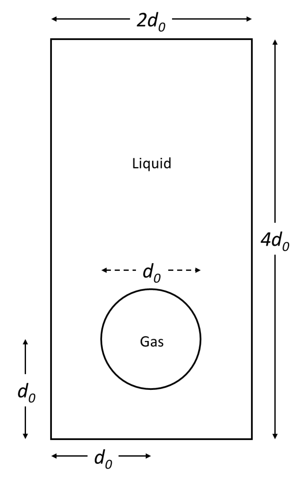
We consider two immiscible fluids in a two-dimensional container, separated by a sharp interface. Initially, both fluids are at rest, and, due to buoyancy effects, the lighter (heavier) fluid is naturally placed on top (bottom) of the container as shown in Figure 1.
Both fluids are Newtonian, incompressible, and immiscible, and their physical properties are constant. The fluid at the top side of the container has density and dynamic viscosity ρ t and μ t , respectively, while the fluid in the bottom side has density and dynamic viscosity ρ b and μ b , respectively. The vertical axis z is aligned with the gravity acceleration g. The container is submitted to an oscillating vertical external force resulting in a total variable acceleration a in the vertical direction as shown in Equation (1),
a = g + a f c o s ( ω t ) ,
where a f and ω are the amplitude and angular frequency of the variable component of the acceleration, respectively.
To describe the dynamics of these fluids, we consider the Navier–Stokes equations for both fluids in laminar flow regime:
· u = 0
ρ u t + · ( u u ) = p + · μ u + u T + ρ g + ρ f s
where ρ and μ are the local fluid density and dynamic viscosity, respectively, p is the pressure, u is the velocity field, g is the gravitational acceleration, and f s takes into account the surface tension effects between the two fluids.
We compare the results obtained with the Phase-Field, Front-Tracking, Volume-Of-Fluid, and Element-based-Volume-of-Fluid schemes after numerically solving Equations (2) and (3). In all the considered schemes, the domain is decomposed into a number of elementary cells. The two fluids are separated by an interface that is determined by either: (a) a function ϕ that changes its values between two extreme values (for example −1 and 1 or between 0 and 1), the value representing the location of the interface being a specific value (e.g., ϕ = 0 or ϕ = 0.5), or (b) the location of a discrete set of points or markers that allow for reconstructing the interface when they are connected. In either case, a subset of cells are traversed by the interface and there the physical properties, density, and viscosity are determined so that their value is proportional to the fluid volumetric fraction of each fluid in the cell.
The boundary conditions for the system of Equations (2) and (3) are: (a) the upper and the lower boundaries are non-slip boundaries and (b) the left and right boundaries are periodic boundaries. Depending on the selected numerical scheme, a different approach is followed to account for interfacial effects. For the sake of completeness, a simplified version of each scheme is presented.

2.1. Front Tracking Scheme

Oliva [22] developed an in-house code, hereafter referred to as F T S , based on the Front Tracking method. His implementation follows the single-field formulation proposed by Tryggvasson et al. [20,23], where a single set of conservation equations is used with the addition of a marker function that identifies the fluids. The discretization of the Navier Stokes equations is performed using the finite volume method in a staggered mesh. The linear momentum conservation equations are solved by the Semi-Implicit Method for Pressure-Linked Equations Revised, SIMPLER, (Patankar [24]). The marker points are advected from the velocity field and then used to reconstruct the marker function and estimate the surface tension force, in the same way as Perinet et al. [14]. When the simulation is performed in a two-dimensional domain, the interface separating the fluids is two-dimensional, and the structure of the front can be handled as a succession of ordered markers connected one after the other. The transfer of information between the front and the staggered grid is done by the smooth weight function proposed by Brackbill and Ruppel [25]. The reconstructing of the marker function is done by first computing its gradient and then integrating it. To maintain accuracy and efficiency, Oliva’s implementation [22] allows for restructuring of the front, involving, inserting, or removing markers in the interface when they get too far away or too close to each other while moving.

2.2. Phase-Field Based Scheme

Phase-field methods model the sharp interface as a diffuse interface. A field variable representing the local presence of each fluid changes in a controlled manner in a finite region of the space. The equation describing this field variable is the Cahn and Hilliard equation [26]. This equation is obtained by considering the time evolution of the fluid volume fraction of each phase, F V F , of the free energy density function of van der Waals. This equation includes the energy gradient (proportional to the local variation of F V F ) and the second bulk energy density (proportional to a function of F V F that considers the local presence rate of each phase, with minimum values at each phase and a maximum at the interface). The effect of surface tension is obtained from the variational derivation of the energy field (Jacmin [27]) and is included in the linear momentum conservation equations as an external force. The conservation equations are then solved simultaneously with the Cahn–Hilliard equation to determine the values of the flow variables and the location of the interface separating the fluids.
The numerical scheme consists of using a staggered grid to represent the variables. The advection term of the Cahn–Hilliard equation is discretized by standard second-order finite difference and aliasing is not eliminated. Concerning the discretization of the chemical potential term, it is split in three terms: the fourth order term which is fully implicit discretized while the other two terms (linear and the third order for free energy) are semi-implicit discretized. On the other hand, the Navier–Stokes equations are discretized using a finite difference projection method [28]. For more details, see Takagi and Matsumoto [15]. This scheme is hereafter called P F S .

2.3. Volume of Fluid Scheme

In order to have a different approach than Front Tracking and Phase fields methods to numerically solve the interface motion, we developed another in-house code combining the Finite Volume method to discretize the Navier–Stokes equations and the Volume of Fluid (VOF) method to model dynamics of the two-phase flow [29].
In the implementation of Machado’s [29] VOF scheme, hereafter called V O F S , the governing equations are solved numerically in a staggered grid, using a system of equations for the entire flow field. The different fluids are identified by a marker function that takes different values for each fluid. In the cells where the interface is located, a value proportional to the relative amount of each fluid must be calculated. As the fluids move, the interface separating them changes location. The new locations are calculated by solving a transport equation for the interface that is identified by the gradient of the marker function. Therefore, an accurate calculation of the relative values of the volume of each fluid in each cell where the interface is located and the normal vector to the interface is needed to solve its transport equation with the precision to ensure proper modeling of the flow dynamics. In our combined Finite Volume discretization-Volume of Fluid implementation, we used the Piecewise Linear Interface Calculation, PLIC, to estimate and reconstruct the interface and estimate the volume fraction of each fluid in the cells and the Efficient Least-square Volume-of-fluid Interface Reconstruction Algorithm, ELVIRA [30], to determine the local normal vector in each cell. To model the effects of surface tension, we use the Continuum Surface Force algorithm, or the CSF model, developed by Brackbill et al. [31], in particular the Marker and Cell (MAC) version in which the zero-thickness interface is replaced by a discrete-thickness interface with a finite thickness, which allows for a smooth variation of the marker function. This smoothed function is an interpretation of the interface as a transition zone, where it changes from a sharp jump in physical properties to a smoother or degraded transition, which helps to obtain more accurate results, favoring the stability of the different numerical methods. The time-advance of the algorithm follows these steps: starting from a velocity field, the interface is advected, then the position of the interface is computed by using PLIC reconstruction and the ELVIRA algorithm [30], the surface tension forces are computed by the CSF method, a new field of velocity and pressure is computed for both fluids, and so on.

2.4. ANSYS CFX Scheme

ANSYS-CFX is a commercial software package with several years on the market. Its solver is based on the finite volume method (Element-based Finite Volume Method, EbFVM). Elemental volumes are obtained from the mesh nodes. Each elemental volume is divided into small subvolumes and field variables are interpolated within each subvolume using interpolating functions. Once the equations are integrated, the contribution of all subvolumes is summed to have the elemental volume contribution to the overall solution. It uses the volume of fluid formulation to model flows with several fluids simultaneously. It has been proven in many applications and today is one of the references in commercial software for fluid flows analysis in a variety of applications.
In this work, we use the second order backward Euler scheme for temporal discretization and the High Resolution scheme for spatial discretization. This scheme is the second order of spatial accuracy in general and first order near discontinuities. To model the interface dynamics, we use the homogeneous model. This model computes common fields of all variables except the volume fraction of each phase. The effects of surface tension interactions are considered using the CSF model of Brackbill et al. [31]. More information can be found in the documentation of the software [32]. This scheme is hereafter referred to as E b F V M S .

2.5. Validation and Verification of In-House Codes

The in house codes developed with the Front Tracking and Volume of Fluid schemes were carefully verified to ensure their ability to accurately model the deformable interfaces as well as the motion of the interfaces. This analysis is presented in Appendix A.

3. Results

The comparison between the different methodologies was performed for the linear and nonlinear regimes. The physical domain is rectangular, as shown in Figure 1, with dimensions L x × L z . The boundary conditions considered were: (a) the lower ( z = 0 ) and upper (z = L z ) boundaries are non-slip walls, and (b) the left ( x = 0 ) and right (x = L x ) vertical walls are periodic boundaries (see Figure 1). The numerical domain is discretized by a uniform mesh with N x × N z cells, the size of each cell is Δ x × Δ z with Δ x = L x / N x , and Δ z = L z / N z .
Initially, to properly compare with the results presented by Takagi and Matsumoto [15], in all cases, it was considered that, at t = 0 , both fluids were at rest and separated by a slightly deformed interface. The initial configuration of the interface is:
z = L z 2 + b c o s ( k x )
where b = L z / Δ z and k = 2 π / L x .

3.1. Linear Regime

To study the linear regime, we consider the same four cases as Takagi and Matsumoto [15]. The physical properties of the fluids, gravity acceleration, vertical length, and angular frequency are given in Table 1.
A careful and detailed sensitivity analysis of mesh size and time steps was performed for all schemes for both linear and nonlinear regime; details are presented in Appendix A. The horizontal length was defined as L x = 2 π / k , and the mesh discretization was N x × N z = 128 × 128 for all codes. Time-step was set to Δ t = 2.5 × 10 6 s for all methods.
Table 2 shows the values of the critical acceleration a c for each considered case.
The values of the critical acceleration are very close. The relative differences between these values and those predicted by the linear theory are shown in Table 3.
In all the cases analyzed, some of the schemes show differences with the reference solution of more than 5%. The first one corresponds to the P F S scheme for k = 28 mm 1 . Takagi and Matsumoto [15] argue that this difference would be a consequence of the relatively large value of L x / N x . However, values of a c for all the other schemes are below 1.5% using the same discretization. The cases correspond to k = 48 mm 1 , and k = 73 mm 1 show differences of more than 8%.
Figure 2 shows the time evolution of the interface at x = L x / 2 for three different values of k. Although all schemes are able to describe the motion of the interface, only the P F S scheme shows discrepancies in the first period. In particular, the difference between the numerical predictions of the phase field scheme and the other schemes for k = 94 mm 1 in the first period is remarkable. However, all schemes are capable of accurately describing the dynamics of the interface.

3.2. Nonlinear Regime

Once all the schemes have been validated, we proceed to analyze a case in the nonlinear regime. In the nonlinear regime, the size of the oscillation amplitude of the interface may be larger compared to the linear regime and the possibility of having plume formation and drop ejection if the external forces operate for several periods. We choose the same test case of Takagi and Matsumoto [15], a modification of a test case considered by Wright et al. [7]. The physical and geometrical parameters are described in Table 4.
The interface is slightly deformed at t = 0 according to Equation (4) with b = −0.01 m. The mean gravity acceleration is 0, and the grid discretization is N x × N z = 256 × 256 for all schemes. The time steps for each scheme, 1.18 × 10 2 s, 3.36 × 10 2 s and 1.0 × 10 2 s for the E b F V M S , F T S and V O F S , respectively, were chosen to ensure that the numerical results were independent of the time discretization. This analysis is shown in Appendix A.2.2. There are two important differences between the values of the physical and geometrical parameters between situations considered by Takagi and Matsumoto [15] and Wright et al. [7]. First, the original case of Wright et al. [7] considers an Atwood number, A t = ( ρ b ρ t )/( ρ b + ρ t ) = 0.65, while the case proposed by Takagi and Matsumoto [15] corresponds to A t = 0.1 . Takagi and Matsumoto [15] argue that their P F S scheme cannot cope with Atwood numbers greater than 0.4. The other difference is the size of the physical domain. Wright et al. [7] consider an infinite physical domain in the vertical direction. For these reasons, comparisons between our results and those of Takagi and Matsumoto [15] with numerical results of Wright et al. [7] can only be qualitative. Figure 3 shows the motion of the interface point located at the midpoint of the container, i.e., at L x / 2 . Although the trends of all numerical simulations are similar, there are some important differences between them. First, there is a very close agreement between the results of the F T S , V O F S and E b F V M S schemes with those of Wright et al. [7] in the first two cycles (the curves corresponding to the three schemes are superimposed on each other). For t / T v > 2 , the predictions of these three schemes show the same trends with relative maximum and minimum values at the same time as those of Wright et al. [7].
On the other hand, the results of the phase-field scheme follow the trend of those of Wright et al. [7] but not as closely as the other schemes. In the first oscillation cycle, the predicted motion of the interface midpoint of P F S is in an opposite (downward) direction to the behavior of the other three schemes (upward). Subsequently, the relative maximum and minimum values are delayed compared to Wright et al. [7]. In all three schemes tested in this work, we found the droplet ejection limit very close to t / T v = 4 .

4. Discussion

Comparison between the numerical results of the three numerical schemes Volume of Fluid ( V O F S ), Front-Tracking ( F T S ), and Element-based Finite Volume Method ( E b F V M S ), and those of the phase field scheme [15], show several important differences. First, in the linear regime, although the acceleration threshold values, a c , determined by all schemes are relatively close for all the cases analyzed. However, none of the schemes analyzed were capable of modeling the four cases considered, with relative differences of less than 5% with respect to the reference solutions. For the case k = 28 mm 1 , the P F S scheme shows important relative differences compared to those presented by the other schemes. In the case k = 48 mm 1 , the E b F V M S scheme presents the most important deviations while, in the other two cases analyzed, the V O F S scheme has the worst performance. The F T S , P F S and E b F V M S schemes are below 3% in at least three of the four cases analyzed.
In all cases, simulations were started for fluids at rest. Only the P F S scheme takes time to synchronize with the reference solutions provide by the linear analysis [2]. In particular, the behavior in the subharmonic case k = 94 mm 1 as it is shown in Figure 2 is remarkable.
Concerning the analysis of the nonlinear regime, for the first two periods, the numerical results of F T S , V O F S and E b F V M S are almost identical to those of Wright et al. [7]. Then, for t / T v > 2.3 , the Wright et al. [7] solution separates from the other three schemes (which continue to agree). This behavior is a consequence of the confinement of fluids by the container walls which are located at dimensionless surface elevation h / L x = ± 0.5. This effect is not appreciable in Wright et al. [7] because their physical domain is infinite in the vertical direction. However, the differences between the prediction of the P F S scheme and the other schemes are appreciable. The surface elevations predicted by the P F S scheme are lower in the first period than those of the vortex-sheet method of Wright et al. [7] and the three schemes developed in this work. Next, for P F S , the interface position at the middle of the tank grows while it goes down with our three schemes (for 1 < t / T v < 2.3 ). After t / T v > 2.3 P F S , minimum and maximum values are significantly different from all the other considered schemes and the solutions of Wright et al. [7].
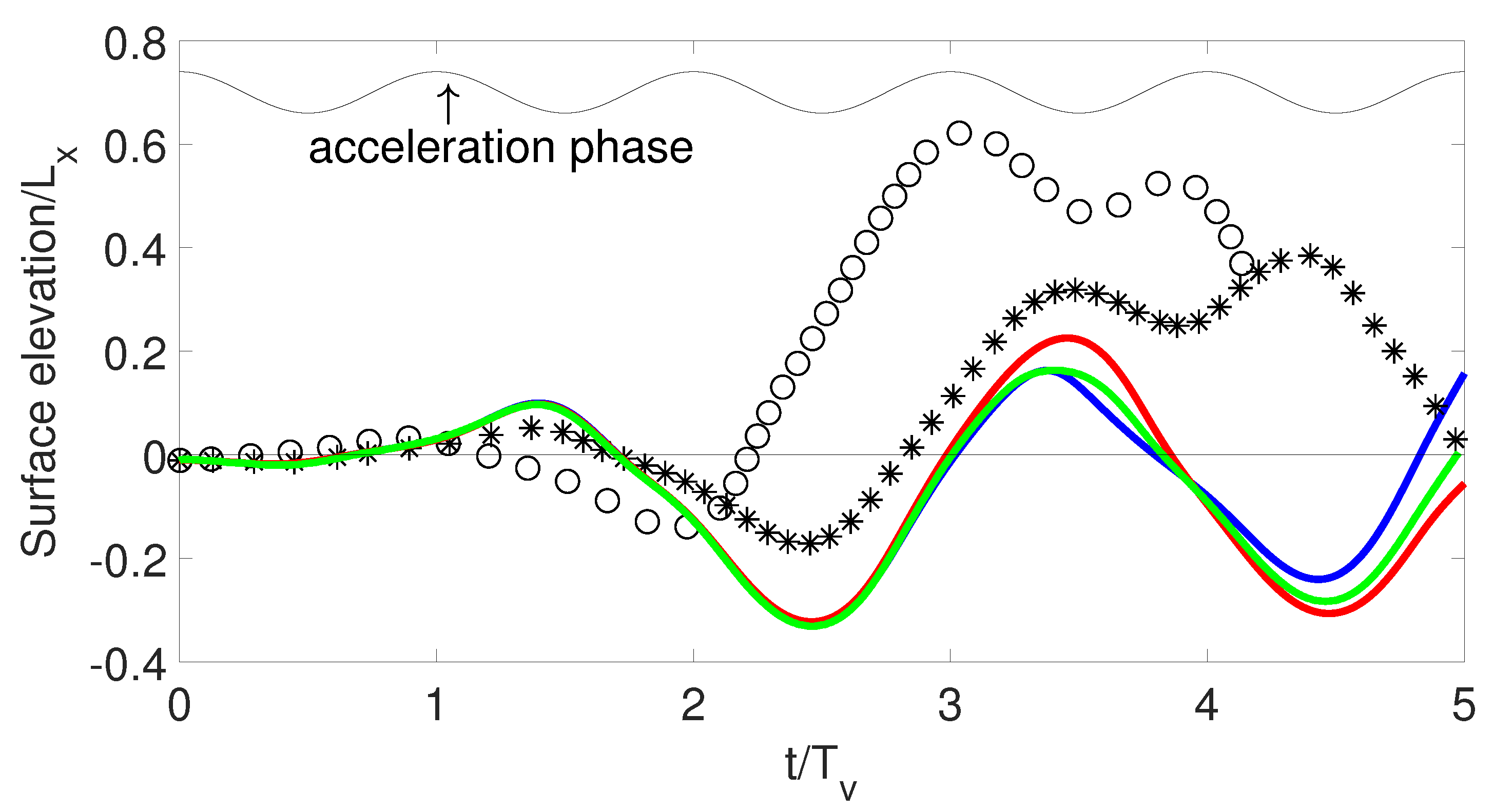
To check the possible causes of this behavior, we performed a last simulation considering that the oscillating acceleration phase was opposite to that considered by Wright et al. [7]. The evolution of the interface midpoint position is presented in Figure 4.
Except for the simulations of Wright et al. [7], the trends of all numerical simulations are the same. Moreover, in the first period, for very small amplitudes, the agreement between all simulations is remarkable as it is shown in Figure 5. From a qualitative point of view, the effect of this phase change in acceleration is to invert the direction of the inertial force on the interface which now acts in the same direction as the interfacial force, i.e., the interface moves towards the bottom of the container, in the opposite direction compared to the original case. This difference in the behavior of the interface can be appreciated in Figure 5.
For t / T v > 1 , the P F S prediction of the surface elevations diverges from the predictions of other schemes, but the trends are similar, the relative minimum and maximum values occur almost at the same time up to t / T v 3.5 . However, from a quantitative point of view, numerical predictions of the P F S -scheme present important differences with the other three schemes considered. Moreover, Figure 4 shows some important differences in surface elevation of the interface midpoint predicted by the F T S and V O F S schemes are appreciable when t / T v > 3 . Figure 6 shows the shape of the interface for various time instants (the same reported in [15]), and it is evident that, after t / T v > 3 , although the shape of the interface follows the same trend, there are some important differences between the F T S scheme and the V O F S and E b F V M S schemes. Figure 6 includes results from [15] even though the direction of acceleration is reversed for illustrative purposes only.
In the search for possible explanations to the difficulties encountered in numerical modeling of Faraday instability, we compare the different time scales involved with the forces present could give some ideas for future work. A dimensional analysis considering the different forces involved (gravitational, viscous, and interfacial tension) leads to the following time scales: t g = ( λ / g ) 1 / 2 , t μ = ( λ 2 ρ / μ ) and t σ = ( λ 3 ρ / σ ) 1 / 2 , where λ is a reference length (wavelength or physical domain length), ρ and μ are the average densities and viscosities, respectively, σ is the surface tension, and g is the maximum value of the modified gravity acceleration. Table 5 shows the values of these scales in all cases analyzed.
The time scale associated with gravity is at least one order of magnitude smaller with respect to the other two time scales in the linear regime simulations and is even three orders of magnitude in the nonlinear regime. Consequently, the difficulty in numerically simulating this problem may lie in solving all these time scales with the necessary accuracy. Consequently, an analysis should be performed using numerical schemes with higher temporal accuracy or based on other formulations such as the use of adaptive meshing at fluid interface.

5. Conclusions

In this work, a comparison is made between different numerical schemes to solve the Navier–Stokes equations for modeling the Faraday instability. Results calculated using the phase field scheme were reviewed from several test cases, in the linear and nonlinear regimes, for the Faraday instability. All cases were modeled using three different codes based on numerical schemes developed from Front Tracking and Volume of Fluid methods and a commercial ANSYS-CFX software developed from a variant of Volume of Fluid methods. The comparison was based on predictions about the evolution of the interface shape or the dynamics of a particular interface point.
Although the numerical predictions in a linear regime are relatively close, some differences between them can be appreciated. In particular, in all cases, for some numerical schemes, the value of the critical acceleration magnitude is not so close to the reference inviscid solution. Moreover, in a linear regime, the P F S scheme requires extra time compared to other schemes to synchronize with the corresponding standing wave in sub-harmonic cases.
In the nonlinear regime, the differences between the numerical solutions for the test case were largest between the P F S scheme and all other schemes considered. Moreover, the excellent agreement between the solutions obtained by the F T S and V O F S schemes and the remarkable quantitative agreement with the reference inviscid solution in the low amplitude time range allow us to conclude that the use of phase-field methods for modeling Faraday instability should be revisited. This is evident in the variant of the nonlinear case (with a reversed phase of the oscillating acceleration), which shows that the trends of all numerical schemes are the same from a qualitative point of view, but some minor but distinguishable differences are observed in the shape of the interfaces by the three different schemes tested.
Consequently, despite the important coincidences between the results obtained between some schemes, some results for both the linear and nonlinear regimes need to be clarified in order to establish a reference solution of Faraday instability. A further study is needed that considers the influence of fluid viscosities, different boundary conditions on the top and bottom walls to make a more reasonable comparison with inviscid solutions, a sensitivity analysis of mesh density and physical domain size, and the use of more accurate temporal schemes. This topic will be considered in future work.

Author Contributions

Conceptualization, A.B. and D.L.; methodology, D.L. and A.B.; software, R.O., D.M. and A.B.; validation, R.O., D.M. and A.B.; formal analysis, D.L. and A.B.; investigation, R.O. and D.M.; resources, Institut Polytechnique de Toulouse, Universidad Austral de Chile; writing—original draft preparation, A.B.; writing—review and editing, D.L., R.O. and D.M.; supervision, D.L. and A.B.; project administration, A.B.; funding acquisition, D.L. and A.B. All authors have read and agreed to the published version of the manuscript.

Funding

This research was funded by the project VIDCA-Innoving 2030 Nº INS-ING-2020-01 A. Blanco of the Universidad Austral de Chile.

Institutional Review Board Statement

Not applicable.

Informed Consent Statement

Not applicable.

Data Availability Statement

Not applicable.

Conflicts of Interest

The authors declare no conflict of interest. The funders had no role in the design of the study; in the collection, analyses, or interpretation of data; in the writing of the manuscript, or in the decision to publish the results.

Abbreviations

The following abbreviations are used in this manuscript:
A t Atwood number, ( ρ b ρ t )/( ρ b + ρ t )
aTotal acceleration
a c Critical amplitude of oscillating acceleration
a f Amplitude of oscillating acceleration
d 0 Bubble diameter
E b F V M S Element based Finite Volume Method scheme
E o Eötvös number, ρ l U g 2 d 0 / σ
f s Interfacial tension force
F T S Front-tracking scheme
F V F Fluid Volumetric fraction
gGravitational acceleration
pPressure
R e Reynolds number, ρ l U g d 0 / μ l
tTime
t 0 Reference time scale in the validation case
T v Period (2 π / ω )
u Velocity field
U g Reference velocity scale in the validation case
V O F S Volume of Fluid scheme
x , z Horizontal and vertical cartesian coordinates
Greek symbols
ρ Fluid density
μ Fluid viscosity
ω Angular oscillating frequency
P F S Phase field scheme
σ Surface tension
Subscripts
bBottom
tTop

Appendix A. Verification of In-House Codes and Sensitivity Grid Analysis

Appendix A.1. Verification of In-House Codes

Both in-house codes, F T S and V O F S , were validated using the benchmark case 1 for a two-phase flow proposed by Hysing et al. [33]. This case models the ascent due to gravity effects of an initially 2D circular gas bubble of diameter d 0 surrounded by a liquid placed in a closed container whose size is 2 d 0 × 4 d 0 . The coordinate reference frame is placed in the lower left corner of the physical domain, and the bubble is initially at position ( d 0 , d 0 ). Figure A1 shows the physical domain and the initial fluid configuration.
Figure A1. Physical domain and initial configuration for a verification test case.
Processes 09 00948 g0a1
To define the physical properties of fluids, the diameter d 0 , velocity U g = g d 0 , and time t 0 = d 0 / U g are the references scale for length, velocity, and time, respectively, and g is the acceleration of gravity. The subscripts l and g correspond to the liquid and gas phases, respectively; the Reynolds and Eötvös numbers are defined as R e = ρ l U g d 0 / μ l and E o = ρ l U g 2 d 0 / σ , respectively. The physical parameters and dimensionless numbers (in terms of the defined references scales) defining the test case are given in Table A1.
Table A1. Physical parameters and dimensionless numbers defining the test case.
Re Eo ρ l / ρ g μ l / μ g σ g ρ l ρ g μ l μ g
( ) ( ) ( ) ( ) (N/m) ( m / s 2 ) ( kg / m 3 ) ( kg / m 3 ) (Pa·s)(Pa·s)
3510101024.50.981000100101
The boundary conditions are: (a) no-slip condition on upper and lower boundaries and (b) free-slip condition on the vertical walls. The numerical domain is discretized by a uniform mesh of 80 × 160 cells. The bubble center-of-mass velocity in the interval between t = 0 s and t = 3 s and the bubble shape at t = 3 s were compared. Figure A2 shows the comparison between the numerical predictions of F T S and V O F S and the benchmark case.
Figure A2. Verification test: Rise velocity and bubble shape for test case 1 of Hysing et al. [33] (o) TP2D [33], (*) V O F S (this work), () F T S (this work).
Processes 09 00948 g0a2
The numerical solutions obtained by the F T S and V O F S codes are numerically the same for both the ascent rate and the bubble shape, with respect to each other and when compared with the three models tested in Hysing et al. [33]. Only the TP2D (a code based on finite-element discretizations for incompressible flow of immiscible fluids with the level set method [33]) model results are shown. This agreement between all numerical results allows us to ensure that the interface effects on the flow dynamics are well taken into account for both codes. Moreover, since ANSYS-CFX is a software that has been used for several decades in countless numerical simulations for multiphase flows, no verification was performed to check its capabilities. This assumption was confirmed by analyzing the Faraday instability in the linear regime.

Appendix A.2. Sensibility Grid Analysis

To assure that the spatial and temporal discretization allow for obtaining results with the required accuracy, a detailed analysis of the size grid elemental volumes and the time-steps was performed, for both linear and nonlinear cases. We choose as reference grids and time-steps those used by Takagi and Matsumoto [15]. Depending on the flow regime (linear or nonlinear), different sizes of elemental grid volumes and time-steps were tested.

Appendix A.2.1. Spacial and Time Steps Discretization: Linear Regime

The phase-field scheme uses a 128 × 128 uniform grid in both directions to study the linear regime. To analyze the sensibility to the spacial grid discretization in the linear regime, each numerical scheme was tested using grids ranging in sizes from 32 × 32 to 128 × 128. The test case was chosen as the one corresponding to standing waves for k = 28 mm 1 , where the phase field scheme obtained the worst results. To analyze grid convergence, the values of a c / g obtained for each grid were compared. Table A2, Table A3 and Table A4 show a c / g and the relative difference with the finest considered grid, 128 × 128, for each scheme.
Table A2. Spacial grid size sensibility analysis of a c / g for E b F V M S in the linear regime.
Grid Size128 × 12896 × 9664 × 6448 × 4832 × 32
a c / g 4.354.354.354.434.57
Δ ( % ) 00.000.001.845.06
Table A3. Spacial grid size sensibility analysis of a c / g for F T S in the linear regime.
Grid Size128 × 12896 × 9664 × 6448 × 4832 × 32
a c / g 4.364.374.384.404.49
Δ ( % ) 00.230.460.922.98
Table A4. Spacial grid size sensibility analysis of a c / g for V O F S in the linear regime.
Grid Size128 × 12896 × 9664 × 6448 × 4832 × 32
a c / g 4.434.434.434.514.56
Δ ( % ) 00.000.001.812.93
Numerical tests show that grids denser than 64 × 64 were able to produce results independent of the size of the grid elements sizes for all tested schemes. In order to have the same grid as Takagi and Matsumoto [15], we chose a 128 × 128 grid to compute all the linear cases considered.
To check the effect of the time step size on the numerical results, we take the same value as [15] as reference, i.e., Δ t 0 = 2.5 × 10 6 s in a 128 × 128 grid. Table A5, Table A6 and Table A7 show the values of a c / g for each numerical scheme as a function of time-steps.
Table A5. Time steps’ sensibility analysis of a c / g for E b F V M S in the linear regime.
Δ t   ( s ) 2.5 × 10−68.0 × 10−51.6 × 10−42.4 × 10−43.2 × 10⁻⁴
a c / g 4.354.354.354.364.37
Δ ( % ) 00.000.000.230.46
Table A6. Time steps’ sensibility analysis of a c / g for F T S in the linear regime.
Δ t ( s ) 2.5 × 10−68.0 × 10−51.6 × 10−42.4 × 10−43.2 × 10⁻⁴
a c / g 4.364.364.374.374.38
Δ ( % ) 00.000.230.230.46
Table A7. Time steps’ sensibility analysis of a c / g for V O F S in the linear regime.
Δ t ( s ) 2.5 × 10−65.0 × 10−67.5 × 10−61.0 × 10−5
a c / g 4.434.414.384.35
Δ ( % ) 0−0.45−1.13−1.81
From the obtained values of a c / g , it is evident that, for all analyzed time step values, the F T S and E b F V M S schemes converge while V O F S requires time step values less than 1.0 × 10 5 s. The three schemes converge for the value of Δ t = 2.5 × 10 6 s used by [15]. In this work, for the cases in the linear regime, we keep the same value as [15], Δ t = 2.5 × 10 6 s.

Appendix A.2.2. Spacial and Time-Step Discretization: Nonlinear Regime

The phase-field scheme uses a 256 × 256 grid to study the nonlinear regime. To analyze the sensibility with the spacial grid discretization in the nonlinear regime, each numerical scheme was tested using grids whose sizes were between 32 × 32 and 256 × 256. The Takagi and Matsumoto [15] case whose physical and geometrical parameters are described in Table 4, and the values of surface elevation shown in Figure 3 were chosen as the test case. The parameters to analyze convergence of grid size and time step were the maximum value of the surface elevation/ L x and its corresponding t/ T v value (around t/ T v = 3 in Figure 3). Table A8, Table A9 and Table A10 show the values of maximum surface elevation/ L x and its t/ T v corresponding value, respectively, for each numerical scheme as a function of grid size.
Table A8. Spacial grid sensibility analysis for the nonlinear regime: maximum value of surface elevation/ L x , its time location t/ T v , and their relative difference compared to 256 × 256 grid for  E b F V M S .
Grid Size256 × 256192 × 192128 × 12896 × 9664 × 64
Surface elevation/ L x 0.4120.4110.4100.4060.403
Δ ( % ) 0−0.24−0.49−1.46−2.18
t/ T v 2.9962.9942.9942.9942.987
Δ ( % ) 0−0.07−0.07−0.07−0.30
Table A9. Spacial grid sensibility analysis for the nonlinear regime: maximum value of surface elevation/ L x , its time location t/ T v , and their relative difference compared to 256 × 256 grid for F T S .
Grid Size256 × 256192 × 192128 × 12896 × 9664 × 64
Surface elevation/ L x 0.4130.4120.4140.4140.413
Δ ( % ) 0−0.240.240.240.00
t/ T v 2.9942.9942.9942.9942.994
Δ ( % ) 00.000.000.000.0
Table A10. Spacial grid sensibility analysis for the nonlinear regime: maximum value of surface elevation/ L x , its time location t/ T v , and their relative difference compared to 256 × 256 grid for V O F S .
Grid Size256 × 256192 × 192128 × 12896 × 9664 × 64
Surface elevation/ L x 0.4160.4160.4150.4150.415
Δ ( % ) 00.00−0.24−0.24−0.24
t/ T v 2.9992.9942.9942.9942.994
Δ ( % ) 0−0.17−0.17−0.17−0.17
Numerical tests show that, for grids denser than 128 × 128, all schemes converge. However, to preserve the same spatial resolution as Takagi and Matsumoto [15], we choose a 256 × 256 grid to perform our simulations. To test the effects of the size of time-steps, we test different time steps for each scheme. We perform the test in a 256 × 256 grid. Table A11, Table A12 and Table A13 show the maximum value of the surface elevation/ L x and its corresponding t/ T v value, for each scheme.
Table A11. Time step sensibility analysis for the nonlinear regime: maximum value of surface elevation/ L x , its time location t/ T v , and their relative difference compared to Δ t ( s )  = 1.18 × 10 3 s for  E b F V M S .
Δ t ( s ) 1.18 × 10−31.18 × 10−21.18 × 10⁻¹
Surface elevation/ L x 0.4120.4120.413
Δ ( % ) 00.000.24
t/ T v 2.9962.9962.992
Δ ( % ) 00.00−0.13
Table A12. Time step sensibility analysis for the nonlinear regime: maximum value of surface elevation/ L x , its time location t/ T v , and their relative difference compared to Δ t ( s )  = 3.36 × 10 2 s for  F T S .
Δ t ( s ) 3.36 × 10−26.72 × 10−21.34 × 10⁻¹
Surface elevation/ L x 0.4130.4120.412
Δ ( % ) 0−0.24−0.24
t/ T v 2.9942.9912.989
Δ ( % ) 0−0.10−0.17
Table A13. Time step sensibility analysis for the nonlinear regime: maximum value of surface elevation/ L x , its time location t/ T v , and their relative difference compared to Δ t ( s )  = 1.0 × 10 2 s for  V O F S .
Δ t ( s ) 1.0 × 10−22.0 × 10−24.0 × 10⁻²
Surface elevation/ L x 0.4150.4150.419
Δ ( % ) 00.000.96
t/ T v 2.9942.9942.993
Δ ( % ) 00.00-0.03
From the obtained values of the maximum values of surface elevation/ L x and its corresponding value of t/ T v for each Δ t , it is observed that convergence was achieved for each scheme by choosing time step values equal to 1.18 × 10 2 s, 3.36 × 10 2 s and 1.0 × 10 2 s for the E b F V M S , F T S and V O F S , respectively.

References

  1. Roy, A.; Govindarajan, R. An Introduction to Hydrodynamic Stability. In Rheology of Complex Fluids; Springer: New York, NY, USA, 2010; pp. 131–147. [Google Scholar]
  2. Kumar, K.; Tuckerman, L.S. Parametric instability of the interface between two fluids. J. Fluid Mech. 1994, 279, 49–68. [Google Scholar] [CrossRef] [Green Version]
  3. Rayleigh, L. XXXIII on maintained vibrations. Lond. Edinb. Dublin Philos. Mag. J. Sci. 1883, 15, 229–235. [Google Scholar] [CrossRef] [Green Version]
  4. Li, Y.; Umemura, A. Threshold condition for spray formation by Faraday instability. J. Fluid Mech. 2014, 759, 73–103. [Google Scholar] [CrossRef]
  5. Liu, F.; Kang, N.; Li, Y.; Wu, Q. Experimental investigation on the atomization of a spherical droplet induced by Faraday instability. Exp. Therm. Fluid Sci. 2019, 100, 311–318. [Google Scholar] [CrossRef]
  6. Chen, P.; Luo, Z.; Güven, S.; Tasoglu, S.; Ganesan, A.V.; Weng, A.; Demirci, U. Microscale assembly directed by liquid-based template. Adv. Mater. 2014, 26, 5936–5941. [Google Scholar] [CrossRef] [Green Version]
  7. Wright, J.; Yon, S.; Pozrikidis, C. Numerical studies of two-dimensional Faraday oscillations of inviscid fluids. J. Fluid Mech. 2000, 402, 1–32. [Google Scholar] [CrossRef]
  8. Kull, H.J. Theory of the Rayleigh-Taylor instability. Phys. Rep. 1991, 206, 197–325. [Google Scholar] [CrossRef]
  9. Brouillette, M. The Richtmyer-Meshkov instability. Annu. Rev. Fluid Mech. 2002, 34, 445–468. [Google Scholar] [CrossRef] [Green Version]
  10. Faraday, M. On the forms and states assumed by fluids in contact with vibrating elastic surfaces. Phil. Trans. R. Soc. Lond. 1831, 52, 319–340. [Google Scholar]
  11. Charru, F. Hydrodynamic Instabilities; Cambridge Texts in Applied Mathematics: Cambridge, UK, 2011. [Google Scholar]
  12. Miles, J.; Henderson, D. Parametrically forced surface waves. Annu. Rev. Fluid Mech. 1990, 22, 143–165. [Google Scholar] [CrossRef]
  13. Kumar, K. Linear theory of Faraday instability in viscous liquids. Proc. R. Soc. Lond. A 1996, 452, 1113–1126. [Google Scholar]
  14. Périnet, N.; Juric, D.; Tuckerman, L. Numerical simulation of Faraday waves. J. Fluid Mech. 2009, 635, 1–26. [Google Scholar] [CrossRef] [Green Version]
  15. Takagi, K.; Matsumoto, T. Numerical simulation of two-dimensional Faraday waves with phase-field modelling. J. Fluid Mech. 2011, 686, 409–425. [Google Scholar] [CrossRef] [Green Version]
  16. Jiang, L.; Perlin, M.; Schultz, W.W. Period tripling and energy dissipation of breaking standing waves. J. Fluid Mech. 1998, 369, 273–299. [Google Scholar] [CrossRef] [Green Version]
  17. Takagi, K.; Matsumoto, T. Numerical simulation of Faraday waves oscillated by two-frequency forcing. Phys. Fluids 2015, 27, 032108. [Google Scholar] [CrossRef] [Green Version]
  18. Blanco, A. Quelques Aspects de L’écoulement d’un Fluide Visqueux Autour D’une Bulledéformable. Ph.D. Thesis, Institut National Polytechnique de Toulouse, Toulouse, France, 1995. (In French). [Google Scholar]
  19. Scardovelli, R.; Zaleski, S. Direct numerical simulations of gas-liquid multiphase flows. Annu. Rev. Fluid Mech. 1999, 31, 567–603. [Google Scholar] [CrossRef] [Green Version]
  20. Tryggvason, G.; Scardovelli, R.; Zaleski, S. Direct Numerical Simulations of Gas-Liquid Multiphase Flows; Cambridge University Press: Cambridge, UK, 2011; pp. 1–322. [Google Scholar]
  21. Popinet, S. Numerical models of surface tension. Annu. Rev. Fluid Mech. 2018, 50, 49–75. [Google Scholar] [CrossRef] [Green Version]
  22. Oliva, R.A. Numerical Solution to Navier–Stokes Equations Using Front-Tracking Based Methods. Master’s Thesis, Universidad Simón Bolívar, Caracas, Venezuela, November 2017. (In Spanish). [Google Scholar]
  23. Tryggvason, G.; Bunner, B.; Esmaeeli, A.; Juric, D.; Al-Rawahi, N.; Tauber, W.; Han, J.; Nas, S.; Janz, Y.-J. A front-tracking method for the computations of multiphase flow. J. Comput. Phys. 2001, 169, 708–759. [Google Scholar] [CrossRef] [Green Version]
  24. Patankar, S.V. A calculation procedure for two-dimensional elliptic situations. Numer. Heat Transf. 1981, 4, 409–425. [Google Scholar] [CrossRef]
  25. Brackbill, J.; Ruppel, H. FLIP: A method for adaptively zoned, particle-in-cell calculations of fluid flows in two dimensions. J. Comput. Phys. 1986, 65, 314–343. [Google Scholar] [CrossRef]
  26. Cahn, J.W.; Hilliard, J.E. Free energy of a nonuniform system. III. Nucleation in a two-component incompressible fluid. J. Chem. Phys. 1959, 31, 688–699. [Google Scholar] [CrossRef]
  27. Jacqmin, D. Calculation of two-phase Navier–Stokes flows using phase-field modeling. J. Comput. Phys. 1999, 155, 96–127. [Google Scholar] [CrossRef]
  28. Harlow, F.H.; Welch, J.E. Numerical calculation of time dependent viscous incompressible flow of fluid with free surface. Phys. Fluids 1965, 8, 2182–2189. [Google Scholar] [CrossRef]
  29. Machado, D. Numerical Solution to Navier–Stokes Equations Using VoF Based Methods. Master’s Thesis, Universidad Simón Bolívar, Caracas, Venezuela, November 2019. (In Spanish). [Google Scholar]
  30. Pilliod, J.E., Jr.; Puckett, E.G. Second-order accurate volume-of-fluid algorithms for tracking material interfaces. J. Comput. Phys. 2004, 199, 465–502. [Google Scholar] [CrossRef] [Green Version]
  31. Brackbill, J.U.; Kothe, D.B.; Zemach, C. A Continuum Method for Modeling Surface Tension. J. Comput. Phys. 1992, 100, 335–354. [Google Scholar] [CrossRef]
  32. ANSYS. CFX Solver Theory Guide, 15th Release; ANSYS Inc.: Canonsburg, PA, USA, 2015. [Google Scholar]
  33. Hysing, S.R.; Turek, S.; Kuzmin, D.; Parolini, N.; Burman, E.; Ganesan, S.; Tobiska, L. Quantitative benchmark computations of two-dimensional bubble dynamics. Int. J. Numer. Methods Fluids 2009, 60, 1259–1288. [Google Scholar] [CrossRef]
Figure 1. Schematic distribution of fluids in the two-dimensional container.
Processes 09 00948 g001
Figure 2. Comparison of the interface position at x = L x / 2 in linear regime cases. (∘) Linear analysis [15], (∗) P F S [15], () E b F V M S (this work), () F T S (this work), () V O F S (this work).
Processes 09 00948 g002
Figure 3. Comparison of different approaches in the nonlinear regime: surface elevation at the midpoint. (o) Wright et al. [7], (*) P F S [15], () E b F V M S (this work), () F T S (this work), () V O F S (this work).
Processes 09 00948 g003
Figure 4. Comparison of different approaches in the nonlinear regime: surface elevation at the midpoint-inverted acceleration phase. (o) Wright et al. [7], (*) P F S [15], () E b F V M S (this work), () F T S (this work), () V O F S (this work).
Processes 09 00948 g004
Figure 5. Initial dynamics of interface midpoint surface elevation after acceleration phase. (o) Wright et al. [7], (*) P F S [15], () E b F V M S (this work), () F T S (this work), () V O F S (this work).
Processes 09 00948 g005
Figure 6. Comparison of the interface shape evolution—Nonlinear case with inverted acceleration. () P F S [15], () F T S (this work), () E b F V M S (this work), () V O F S (this work).
Processes 09 00948 g006
Table 1. Physical parameters defining linear test cases.
ρ b ρ t μ b μ t σ g L z ω
(kg/m3)(kg/m3)(Pa·s)(Pa·s)(N/m)(m/s2)(m)(s−1)
519.933415.6673.908 × 10−53.124 × 10−52.181 × 10−69.80662.31 × 10−4200 π
Table 2. Comparison of critical amplitude values a c /g in the linear regime.
k (mm−1)Linear Theory P F S F T S V O F S E b F V M S
284.374.654.364.434.35
4812.5012.5012.1711.7513.55
7328.5028.4027.6525.2529.20
9451.0050.0048.0648.0049.90
Table 3. Relative difference between computed critical amplitude values a c /g and linear theory predictions.
k (mm−1) P F S F T S V O F S E b F V M S
286.41−0.21.37−0.46
480.00−2.64−6.008.40
73−0.35−2.98−11.402.46
94−1.96−5.76−5.88−2.16
Table 4. Physical parameters defining the nonlinear test case.
ρ b ρ t μ b μ t σ L x L z a f ω
(kg/m3)(kg/m3)(Pa·s)(Pa·s)(N/m)(m)(m)(m/s2)(s−1)
1000818.180.20.20.072110.090.26728
Table 5. Comparison of time scales in linear and nonlinear cases.
Case t g (s) t μ (s) t σ (s)
L i n e a r k = 28 mm 1 0.00400.66790.0491
L i n e a r k = 48 mm 1 0.00230.17000.0176
L i n e a r k = 73 mm 1 0.00150.09870.0117
L i n e a r k = 94 mm 1 0.00100.05940.0080
N o n L i n e a r 3.334545355
Publisher’s Note: MDPI stays neutral with regard to jurisdictional claims in published maps and institutional affiliations.

