Abstract
Due to the inadequate pre-dispersion and high dust concentration in the grading zone of the turbo air classifier, a new rotor-type dynamic classifier with air and material entering from the bottom was designed. The effect of the rotor cage structure and diversion cone size on the flow field and classification performance of the laboratory-scale classifier was comparatively analyzed by numerical simulation using ANSYS-Fluent. The grinding process performance with an industrial classifier was also tested on-site. The results revealed that an inverted cone-type rotor cage is more suitable for the under-feed classifier. When the rotor cage’s top-surface diameter to bottom-surface diameter ratio was too large or too small, the radial velocity and tangential velocity at the outer surface of the rotor cage greatly fluctuated. Furthermore, the diameter of the diversion cone also affected the axial velocity and radial velocity of the flow field. Models T-C(1-0.8) and T-D(1-0.7) were determined as the best rotor cage structures. Under stable operating conditions, the classification efficiency of the industrial classifier was 87% and the sharpness of separation was 0.58, which meet the industrial requirements for classification efficiency and energy consumption. This present study provides theoretical guidance and engineering application value for air classifiers.
1. Introduction
Powder classification technology is one of the essential parts of the powder preparation process. Powder is widely used in the fields of building materials, metallurgy, chemical industry, and medicine, due to its large specific surface area, low melting point, and good activity, significantly promoting the development of powder classification technology [1,2]. The turbo air classifier has become the mainstream powder classification equipment with simple structure, controllable product granularity, and other advantages. With the development of materials science, powder classification technology has exhibited a trend of ultrafine and narrow-grading [3]. Therefore, the development of more efficient and energy-conserving classifying equipment has become one of the hot spots.
After the industrial application of turbo air classifiers (O-Sepa classifier), especially with the advent of large-sized classifiers, many problems arose because of the limitations of the structure itself. This affected the classification efficiency and increased the system energy consumption [4,5]. Three examples follow. (1) Uneven material dispersion—since the limitations of the structure, the number of feed inlets cannot be increased without limit as the increase of equipment processing capacity, this resulted in uneven materials on the spreading disk. Hence, a thicker material curtain would appear at the feed inlet, affecting material dispersion and reducing the classification efficiency. (2) High concentration of particles in the classification area—after grinding, the particles will all enter the grading area, which would cause high dust concentration in the powder selection area, increasing the chance of collision between particles and reducing the sharpness of separation. (3) Unequal inlet air volumes and uneven internal air pressure—turbo air classifiers use two air inlets of unequal size, with different air volumes resulting in uneven air pressure inside the equipment and increased energy consumption. Furthermore, the volute structure of the turbo air classifier will lead to the local accumulation of materials. In recent years, researchers have mainly improved the classification theory [6,7,8,9], studied its internal flow field [10,11,12], improved the structure of the classifier [13,14], and optimized the operating parameter [15,16,17], in order to improve the flow field distribution characteristics inside the turbo air classifier and enhance the classification performance. However, no study has been conducted to solve the problems of uneven material dispersion and high dust concentration in turbo air classifiers. Therefore, this paper designs a new rotor-type dynamic classifier with air and material entering from the bottom, replacing the turbo air classifier when used in combination with the V-type static separator. The structure is shown in Figure 1a. The V-type static separator intercepts the coarse particles (d > 100 μm) after ball milling. Other particles of different sizes enter the dynamic classifier have a time difference, which effectively reduces the material concentration in the dynamic classifier. Furthermore, the dynamic classifier adopts wind feeding. The airflow pre-dispersed the particles before classification, making the material fully diffused in the classification area.
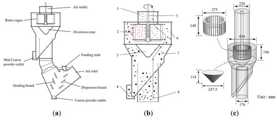
Figure 1.
The new high-efficiency three separation classifier: (a) geometry, (b) parts, and (c) dimensions of the new rotor-type dynamic classifier; 1—air and fine outlet, 2—rotor cage, 3—diversion cone, 4—coarse powder outlet, 5—transmission shaft, 6—classification chamber, 7—cone, and 8—feeding and air inlet.
Particle classification mainly occurs at the outer surface of the rotor cage, and the uniform velocity distribution in this area will help keep the cut size constant and improve the sharpness of separation. The rotor cage is the core component of the new rotor-type dynamic classifier. The structure of the rotor cage directly affects the interior flow field and classification performance of the classifier. Hence, a number of researchers have focused on the rotor cage. Huang [18] found that the splitter-style rotor cage can make the tangential velocity and radial velocity distribution at the outer surface of the rotor cage of the turbo air classifier more uniform, which is conducive to reducing the classification particle size and improving the sharpness of separation. Ren [19] designed a rotor cage with a non-radial arc blade to replace the straight-blade rotor cage. The material classification experiment results have proven that the new rotor cage led to a classification accuracy increase of 10.60–40.80% and increased fines yield of 12.50–40.10%. Yu [20] investigated the effect of rotor cage size on the flow field of the turbo air classifier using CFD (Computational Fluid Dynamics) techniques, and the results revealed that too large or too small of the rotor cage outer and inner radius can lead to large fluctuations in the tangential and radial velocities in the classification zone. For the new rotor-type dynamic classifier with air entering from the bottom, the uneven velocity distribution on the outer surface of the cylindrical rotor cage can greatly reduce the sharpness of separation and classification efficiency. However, the inverted conical rotor cage can be an excellent solution this problem.
In order to investigate the influence of the rotor cage and diversion cone structure on the inner flow field of the new rotor-type dynamic classifier, numerical simulations and a comparative analysis of classifiers with different rotor cage structures and diversion cone structures were carried out. The results revealed that the inverted conical rotor cage is more suitable for a classifier with air and material entering from the bottom. The top-surface diameter to bottom-surface diameter ratio of the rotor cage should be neither too large nor too small. In addition, the industrial classifier has put into production and its classification performance tested and discussed.
2. Calculation Methodology
2.1. Equipment Description and Classification Principle
The schematic diagram for the new rotor-type dynamic classifier is shown in Figure 1b. The materials to be classified are carried by air into the classifier from the bottom air inlet (8). A part of the coarse particles entering the classifier is deposited by inertia as coarse powder due to the collision with the guide cone (3). The remaining materials enter the classification chamber under the airflow. In the classifying zone, the airflow and the particles that dispersed in the airflow are driven by the rotor cages (2) and rotate together with the rotor cage at high speed. These particles are subjected to three kinds of forces: gravity, centrifugal force, and air drag force. When the particle size is large, the mass is large. The centrifugal force of the coarse particles is greater than the air drag force, so the coarse particles will escape the carrying effect of the airflow and hit the cylinder wall to lose momentum. Eventually, these are collected by the coarse powder outlet (4). When the particle size is small, the mass is small. Since the centrifugal force of the fine particles is less than the air drag force, they are carried by the airflow through the rotor cage blades and out through the air outlet (1).
The structural features follow:
(a) The feeding adopts air conveyance to induce the materials to fully disperse in the classifier.
(b) The centrifugal force field is used as the classification force field for the classifier. Taking into account the distribution pattern of the gas flow field in the classification chamber, an inverted conical rotor cage is used. The inverted conical rotor cage provides a uniform and stable classification force field within the classification chamber. The material is subjected to the same force near the classifying surface, which ensures that the classifier has a high classification accuracy.
(c) Compared to the turbo air classifier, the transmission shaft only needs to drive the rotor cage to rotate. Thus, the energy consumption of the new classifier is significantly reduced.
(d) The new rotor-type dynamic classifier is widely used. It can be combined with the V-type static separator and used in the tubular ball mill system or used alone with the air-swept grinding system.
2.2. Model Establishment and Mesh Generation
The laboratory-scale classifier geometry model was established using SolidWorks 2019. The model was divided into six main domains: the feeding part, rotor cage, diversion cone part, coarse powder collection area, fine powder collection area, and particle classification area. The geometric parameters of the main structure are shown in Figure 1c. The origin of the coordinates is the center of the top surface of the rotor cage. The rotor cage is an important part of the classifier. A total of 30 radial blades (148 × 2 × 20 mm) were installed evenly across the circumference of the rotor cage. The positive cone rotor cage is clearly unsuitable for an under-feed classifier. Hence, simple cylindrical and inverted conical rotor cages were considered for the present study. If the structure of the rotor cage is changed, the inner edge width of the rotor cage channel is also changed. When the diameter of the rotor cage chassis is less than 137.5 mm, the width between the blades at the bottom of the rotor cage is less than 8 mm. In this case, the fine powder cannot flow out. Furthermore, when the ratio between the top surface and bottom surface of the rotor cage is too large, the rotor cage will rotate unstably at high speed. In the present paper, the prototype-rotor cage-top diameter to bottom diameter ratio was 1:1, and this is defined as T-A(1-1), and so on. Therefore, in addition to the classifier prototype T-A(1-1), the rotor cage models of T-B(1-0.9), T-C(1-0.8), T-D(1-0.7), T-E(1-0.6), and T-F(1-0.5) were established (Table 1). In calculating the different rotor cage structures, it was assumed that the diversion-cone diameter to rotor-cage-chassis diameter ratio was 0.9:1.0, and the height was 114 mm.

Table 1.
Dimensional parameters of the rotor cage model.
For the coarse powder collection area, a tetrahedral grid was used to create the mesh in ANSYS-MESH 19.0 (ANSYS, Canonsburg, PA, USA) software. For the feeding part, rotor cage, diversion cone part, fine powder collection area, and particle classification area, due to the regular structure, hexahedral grids were used to create the mesh in ICEM CFD software. Figure 2 shows an overview of the grid. In order to ensure the accuracy of the calculation results, the grid independence needs to be verified after the grid is divided. Four grid sizes were examined in the same conditions, including 509,583, 1,204,187, 2,105,369, and 3,012,885. Several points were selected to check the velocity field distribution using these four grid sizes. For example, some points in the axial direction (x = 0 mm, y = 136 mm, z = 0~−148 mm) on the surface of the rotor cage were selected. The radial velocity obtained using the four grid sizes is shown in Figure 3. When the number of mesh is greater than 2,105,369, the radial velocity did not significantly change. This means that the calculation results are independent of how the grid is divided. A mesh with 2,105,369 elements was selected to conduct the simulation required in the present study. Table 2 lists the specific grid numbers.
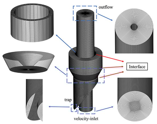
Figure 2.
CFD grid and boundary conditions of the simulated classifier.
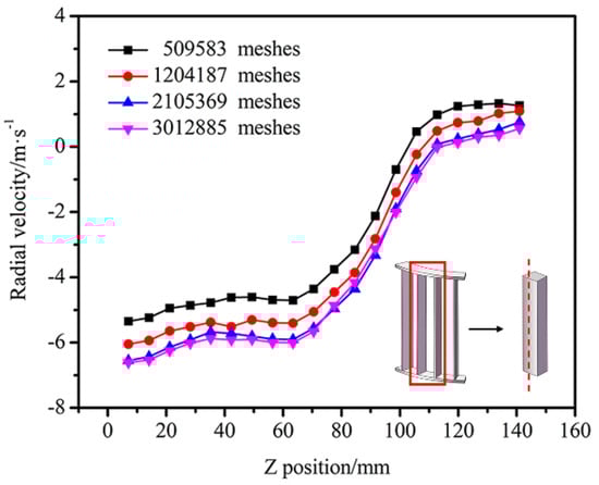
Figure 3.
The radial velocity for four different mesh numbers.
Table 2.
Mesh number of the model and near-wall grid height for the new rotor-type dynamic classifier.
2.3. Mathematical Model
2.3.1. Turbulence Model Description
Three-dimensional steady simulations were performed using ANSYS-FLUENT 19.0 (ANSYS, USA). When the new rotor-type dynamic classifier worked, the internal space was at room temperature, with negative pressure and low-velocity flow. Hence, the air was considered as incompressible flow. For the steady and incompressible fluid flow, the mass and momentum equations are expressed as follows:
where is the fluid velocity, is the position, is the fluid density, is the fluid viscosity, is the static pressure, and is the Reynolds stress term.
Renormalization Group - (RNG -) and Reynolds Stress Model (RSM) can both be used in dynamic classifier flow field simulation [1,8,21]. But RSM is more accurate when calculating flow field in an abruptly changing separation zone. Therefore, it is more suitable for high-speed rotating fluid motion. Sun [22] and Guizani [23] demonstrated that RSM can more completely predict the turbulent structure and pressure drop inside the turbo air classifier, and calculated results were closer to the experimental results. Therefore, in the present paper, the RSM model was used to simulate the turbulent flow in the new rotor-type dynamic classifier. The Reynolds stress equation can be expressed as:
where is the fluctuating velocity to the direction i ( − ), is the velocity to direction i, is the mean velocity to direction i, is the time, is the fluid density, is the positional length, is the fluid viscosity, is the gravitational acceleration, p is the fluid pressure, is alternating symble, is Kronecker delta, and is the rotation tensor; is the coefficient of thermal expansion, defined as , where T is the temperature. Since in this paper the fluid (air) is considered an incompressible fluid, in Equation (3).
2.3.2. Discrete Phase Model
When the particle volume loading rate is very small (10–12%), the particle motion trajectory can be tracked using a discrete phase model (DPM). Zeng [16] provided formulae for the particle volume loading rate () and mass loading rate (). The processing air volume of laboratory-scale classifier is 1000–1700 m3/h. The capacity of the new rotor-type dynamic classifier is 800 kg/h. The calculated particle volume loading rate () ranges from 1.48 × 10⁻⁴ to 2.48 × 10⁻⁴. Therefore, the particle phase inside the classifier is relatively sparse, and the DPM is used to model the air-particle flow inside the classifier. In addition, the effect of particles on the flow field is not considered, and the coupling between the particle phase and the gas phase is considered to be single-phase. By adding particles to the flow field simulated in the continuous phase, the Lagrangian trajectory of the particles can be calculated based on the forces on the particles in the flow field.
The equations for the discrete particles follow:
where is the time, is the fluid phase velocity, is the particle velocity, is the fluid density, is the density of the particle, and is the gravitational acceleration.
is a source term that indicates the presence of additional forces. mainly include the virtual mass forces required to accelerate the fluid around the particle, the forces due to the pressure gradient in the fluid, and the forces on particles that arise by rotation of the reference frame.
is the drag force per unit particle mass:
where is the molecular viscosity of the fluid, is the particle diameter, is the Reynolds number; is the drag coefficient, where ,, and are constants that apply to smooth spherical particles over several ranges of given by Morsi and Alexander [24].
2.3.3. Simulation Conditions
The new rotor-type dynamic classifier has rotating parts inside, and a Multiple Reference Frame model (MRF) was used to couple the moving rotor cage with the surrounding stationary area. The “interface” was used for each part of the grid intersection. The classifier has one inlet and two outlets, and the boundary condition for the air inlet is “velocity inlet”. It is assumed that the air velocity distribution at the air inlet is uniform, and that the direction is normal to the air inlet boundary. The boundary condition for the fine-particle outlet was prescribed as fully developed pipe flow, and treated as ‘‘outflow”. The outlet length was lengthened to prevent backflow. In industrial applications, the coarse powder outlet is usually equipped with a locking air valve, so the boundary condition is “wall”. The rotor cage rotates clockwise around the Z axis. A no-slip boundary condition was used on the wall boundary, and the near wall treatment was a standard wall function. For standard wall function, the wall-adjacent cell centroid should be located within the log-law layer . Table 2 lists the near-wall grid heights of the grid model. The Semi-Implicit Method for Pressure Linked Equations Consistent (SIMPLEC) algorithm was used for pressure-velocity coupling, and Quadratic Upwind Interpolation of Convective Kinematics (QUICK) differential scheme was chosen for convective and diffusion. In this paper, air inlet velocity of 13.5 m/s and a rotor cage rotating speed of 470 rpm were used as the design conditions. For the convenience of the following description, it is referred to as air inlet velocity–rotor cage rotating speed (13.5 m/s–470 rpm). Calcium carbonate (CaCO3) with 2700 kg/m3 was selected as the feed material to be classified in the simulation.
2.3.4. Model Validation
Pressure drop, which is crucial for assessing the energy consumption of the equipment, was adopted as the main parameter for model validation. In order to verify the accuracy of the numerical simulation calculations, the pressure drop between the simulation results and the experimental results was compared. The pressure drop is calculated from the average static pressure difference between the air inlet and air outlet. The measuring instrument used was a U-type manometer with the specification of 3 kPa, and a U-shaped glass tube filled with working liquid (water was chosen because the pressure drop of the equipment is relatively small). One end of the U-shaped tube was connected to the air inlet of the new rotor-type dynamic classifier, and the other end to the air outlet. For pure gas flow, pressure drops from the simulations and experiments were compared and shown in Table 3. The relative errors of both the calculated data and the experimental data are small, within 5%. The correctness of the simulation results is verified.
Table 3.
Comparison of simulated and experimental pressure drop .
3. Simulation Results and Analysis
3.1. Effect of the Rotor Cage Structure on the Classification Performance of the New Rotor-Type Dynamic Classifier
3.1.1. Effect of the Rotor Cage Structure on Velocity Distribution at the Outer Surface of the Rotor Cage
Particle classification mainly occurs in the area near the outer surface of the rotor cage. The cut size () in the separation face can be described by
where is the density of the particle, is the gas density, R is the outer semidiameter of rotor cage, is the drag coefficient, is the radial velocity, and is the tangential velocity. Equation (8) shows that d50 can be kept constant at any position within the grading surface, when the tangential and radial velocities in the classification area are uniformly distributed. In order to investigate the radial velocity and tangential velocity distribution on the outer surface of different rotor cage structures, 20 points were uniformly taken from top to bottom in the axial direction on the outer surface of the rotor cage. Figure 4 shows velocity distribution on the outer surface of the different rotor cage. Figure 5 shows the radial velocity contour of the classifier and the gas pathlines in the classifying chamber.
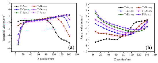
Figure 4.
Velocity distribution on the outer surface of the rotor cage: (a) tangential velocity and (b) radial velocity.
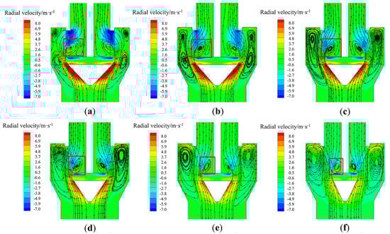
Figure 5.
Comparison of radial velocity contours and gas pathlines in the classifying chamber: (a) T-A(1-1), (b) T-B(1-0.9), (c) T-C(1-0.8), (d) T-D(1-0.7), (e) T-E(1-0.6), and (f) T-F(1-0.5).
As shown in Figure 4a, the tangential velocity is mainly controlled by the speed of the rotor cage. Hence, there is no significant difference in the tangential velocity value. As the height of the rotor cage increases, the tangential velocity decreases, and subsequently increases. Vortices of different sizes form in the lower half of the rotor cage, which lead to the increase in the tangential velocity gradient in the classifying area. Furthermore, a portion of the airflow is thrown out at the upper area of the rotor cage, which accelerates the movement of coarse particles away from the separation zone, and facilitates the reduction in cut size. The top of the cylindrical rotor cage has a low tangential velocity, while the top of the inverted conical rotor cage has a high tangential velocity. For example, the top tangential velocity of T-A(1-1) is −1.79 m/s and the top tangential velocity of T-F(1-0.5) is −5.56 m/s. Therefore, the inverted conical rotor cage is more suitable for classification equipment with air entering from the bottom.
The radial velocity of the flow field was analyzed, and the negative sign indicates the direction towards the center of the rotor cage. Figure 4b shows that the cylindrical rotor cage has the largest radial velocity and the largest velocity gradient on its outer surface. For example, T-A(1-1) has the maximum radial velocity at the top of the rotor cage with a value of −6.8 m/s, and the minimum radial velocity at the bottom of the rotor cage with a value of 0.9 m/s, with a velocity gradient of 7.7 m/s. As the diameter of the rotor cage chassis decreases, the area of the outer surface of the rotor cage becomes larger. The radial velocity and the velocity gradient on the outer surface of the rotor cage both become smaller, with a constant air volume. For example, T-D(1-0.7) has a maximum radial velocity of −3.59 m/s, a minimum radial velocity of 0.85 m/s, with a gradient of 4.44 m/s. When the rotor cage chassis is again reduced, the radial velocity gradient increases. For example, for T-E(1-0.6), the maximum radial velocity is −3.2 m/s, and the minimum radial velocity is 3.1 m/s, with a gradient is 6.3 m/s.
The reasons for the formation are presented in Figure 5. For cylindrical rotor cage, the incidence angle of the airflow into the rotor cage is too large, and part of the airflow will hit the transmission shaft. Due to the reflective effect of the transmission shaft, a vortex is formed underneath the rotor cage. This prevents the airflow from entering the interior of the rotor cage, resulting in an uneven radial velocity distribution at the outer surface of the rotor cage. As the diameter of the rotor cage chassis decreases, the incidence angle of the airflow decreases, and the strength and size of the vortex at the bottom of the rotor cage gradually decreases. The radial velocity distribution in the graded area at the outer edge of the rotor cage is relatively uniform, and the velocity gradient is reduced, for example, as shown in Figure 5c,d for T-C(1-0.8) and T-E(1-0.7). When the rotor cage chassis is too small, the airflow enters the interior mainly from the bottom of the rotor cage due to the negative pressure in the center of the rotor cage. The coarse particles that just enter the powder selection area are dragged inside the rotor cage by the strong airflow dragging force due to their proximity to the center of the cage, and the cut size increases. In summary, T-C(1-0.8) and T-E(1-0.7) radial velocity gradients are relatively small.
In order to analyze the uniformity of the velocity distribution on the outer surface of the rotor cage, the following standard deviation was introduced:
where S is the standard deviation of the velocity distribution, is the number of points examined, is the velocity of each point in the region, and is the average velocity of the region. Four blade areas were selected and positioned as shown in Figure 6.
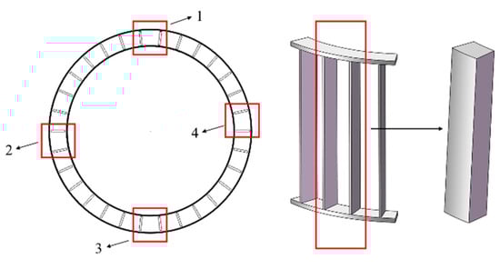
Figure 6.
Location of the sampling points.
Table 4 lists the tangential velocity and radial velocity deviations. T-A(1-1) has a relatively large standard deviation of 2.45 and 1.41 for tangential velocity and radial velocity, respectively. As the diameter of the rotor cage chassis decreased, the standard deviation of the tangential velocity and radial velocity decreased. Furthermore, when the chassis diameter decreased to a certain level, the closer the fluid unit is to the center of the rotor cage, the greater the axial and radial velocity. This resulted in a greater variation in airflow velocity. For example, when the model was changed from T-D(1-0.7) to T-E(1-0.6), the standard deviation of the radial velocity increased from 1.64 to 1.97, and the standard deviation of the tangential velocity increased from 1.09 to 1.31. Therefore, an excessively large or small chassis can lead to uneven velocity distribution. The tangential velocity distribution for T-B(1-0.9) was relatively uniform. However, the radial velocity in the upper region of the classification chamber was larger, increasing the probability for coarse particles entering the interior of rotor cage. Therefore, the standard deviations for the tangential velocity and radial velocity for model T-C(1-0.8) and T-D(1-0.7) are relatively small under the design conditions. These standard deviation results also validate the previous analysis.
Table 4.
Standard deviation comparison of velocity for different rotor cage models.
3.1.2. Effect of the Rotor Cage Structure on Velocity Distribution at the Classification Chamber
In the classifying chamber, the air drag force at the location of the particles determines whether these can move to the vicinity of the rotor cage, and go through the blades. Therefore, eight horizontal lines of different height were selected near the rotor cage to investigate the variation of the drag force in the radial direction. The main work areas for the rotor cage classification were determined by observing the radial velocity distribution of the horizontal lines at different heights. Figure 7 presents the radial velocity distribution for the X = 0 section. The minus sign indicates the direction towards the center of the rotor cage.
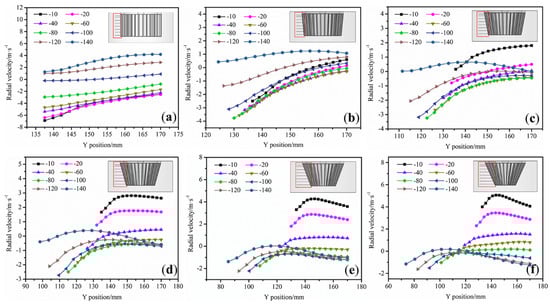
Figure 7.
Radial velocity distribution at different heights in the classifying chamber: (a) T-A(1-1), (b) T-B(1-0.9), (c) T-C(1-0.8), (d) T-D(1-0.7), (e) T-E(1-0.6), and (f) T-F(1-0.5).
The axial direction was analyzed from top to bottom. As shown in Figure 7a, the radial velocity is greatest at a distance of 20 mm from the top of the rotor cage, and this increases as the distance from the rotor cage lessens. The radial velocity reaches a maximum at 136 mm (the outer edge of the rotor cage), after which the velocity decreases due to the centrifugal force generated by the impeller rotation. This means that particles of this height quickly approach the rotor cage. As the height of the rotor cage gradually increases, the radial velocity of the flow field becomes smaller. At 100 mm from the top, the radial velocity is 0 m/s. As the height of the rotor cage continues to increase, the radial velocity becomes positive, and the airflow begins to move in the opposite direction. This means that there is less air drag force at the bottom of the classification chamber, and fewer particles reach the vicinity of the rotor cage. Therefore, the grading area for T-A(1-1) is located in the region at 0–80 mm from the top surface of the rotor cage.
As shown in Figure 7b, there is little difference in the radial velocity near the rotor cage between 10 and 80 mm, and the velocity increases as the distance to the rotor cage lessens. Furthermore, as the height of the rotor cage increases, the radial velocity of the classification chamber increases, and subsequently decreases. At 140 mm from the top of the rotor cage, the radial velocity of the flow field becomes positive, and the flow reverses. Therefore, the graded area of T-B(1-0.9) is located at a distance of 0–120 mm from the top of the rotating cage. The area where the coarse particles collect is mainly at the upper part of the classification chamber. However, the radial velocity in the upper part of the classification chamber is within the range of 3–4 m/s, which causes coarse particles to be carried inside the rotor cage by the airflow, increasing the cut size.
As shown in Figure 7c, the radial velocity changes from positive to negative at 20 mm from the top surface of the rotor cage. In the upper part of the classification chamber, a small portion of the airflow is thrown out of the cage, creating a vortex between the cage and the wall for the secondary sorting of particles. At a distance of 140 mm from the top of the rotor cage, the radial velocity is 0 m/s. Therefore, the grading area for T-C(1-0.8) is located in the region at 20–120 mm from the top of the rotor cage. T-D(1-0.7) and T-C(1-0.8) are similar, with the graded area of T-D(1-0.7) located at 40–120 mm. As seen from Figure 7e,f, the grading positions for T-E(1-0.6) and T-F(1-0.5) are mainly located at the bottom of the rotor cage. These are all graded at a distance of 60–140 mm from the top of the rotor cage. Due to the negative pressure in the center of the rotor cage, the coarse particles that entered the classification zone are carried directly into the interior of the rotor cage by the airflow, increasing the cut size.
In summary, it can be observed that the T-C(1-0.8) and T-D(1-0.7) graded areas are located in the middle of the rotor cage, and have the largest graded areas.
3.1.3. Discrete-Phase Simulated Results and Analysis
In the classification process, the particle movement trajectory can be tracked and visualized, which can visually explain the particle classification mechanism. Therefore, discrete phase model was established in Fluent to simulate the particle trajectory and compare the particle motions for six different rotor cage structures.
Simulation Results and Analysis of Single Particle
The uniformity of the particle concentration distribution on the outer edge of the rotor cage has a relatively large influence on the classification effect. High particle concentrations in local areas increase the probability of collision and aggregation between particles, which will reduce classification accuracy [25]. Therefore, the classification position of different size particles is particularly critical. Figure 8, Figure 9, Figure 10, Figure 11, Figure 12 and Figure 13 present the particle trajectory in the classifier of six different rotor cage structures. The calcium carbonate particle sizes are set at 5, 15, 25, and 35 μm. As seen from Figure 8 and Figure 9, in models T-A(1-1) and T-B(1-0.9), the fine (5 and 15 μm) and coarse particle (25 and 35 μm) classifications are located at the upper half of the rotor cage. The reason for this is that in the under-feed classifier, the incidence angle of the airflow at the entrance to the rotor cage is too large, and a vortex forms below the rotor cage, impeding the flow of air, thereby causing the lower half of the rotor cage to lose its classification function. Hence, the particles gathered in the upper part of the classifying chamber for classification. Increased probability for collision and aggregation between particles resulted in reduced sharpness of separation. As seen from Figure 12 and Figure 13, in models T-E(1-0.6) and T-F(1-0.5), the fine and coarse particle classifications are located at the bottom half of the rotor cage due to the relatively small size of the chassis diameter of the rotor cage and the small distance of the fluid unit from the center of the rotor cage. Hence, the fluid unit is affected more by the negative pressure at the center of the rotor cage, resulting in a large radial velocity in the lower part of the classification chamber. Particles carried by air can easily pass through the blades from the bottom of the rotor cage. In models T-C(1-0.8) and T-D(1-0.7), as shown in Figure 10 and Figure 11, the fine particles (5 and 15 μm) follow the airflow into the rotor cage at the lower part of the classifying chamber, and coarse particles (25 and 35 μm) are graded in the upper part of the classifying chamber. This means a uniform particle concentration distribution on the outer surface of the rotor cage in models T-C(1-0.8) and T-D(1-0.7). Models T-C(1-0.8) and T-D(1-0.7) decrease particle collision and aggregation probability and improve the particle concentration distribution in the classification area.
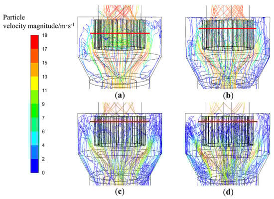
Figure 8.
Trajectories of different size particles in T-A(1-1): (a) d = 5 μm, (b) d = 15 μm, (c) d = 25 μm, and (d) d = 35 μm.
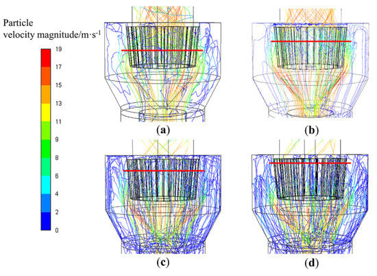
Figure 9.
Trajectories of different size particles in T-B(1-0.9): (a) d = 5 μm, (b) d = 15 μm, (c) d = 25 μm, and (d) d = 35 μm.
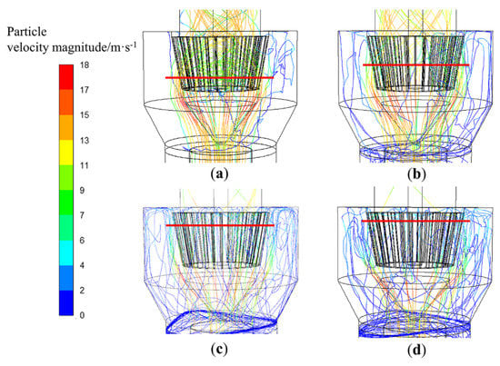
Figure 10.
Trajectories of different size particles in T-C(1-0.8): (a) d = 5 μm, (b) d = 15 μm, (c) d = 25 μm, and (d) d = 35 μm.
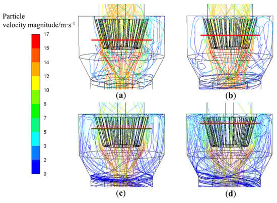
Figure 11.
Trajectories of different size particles in T-D(1-0.7): (a) d = 5 μm, (b) d = 15 μm, (c) d = 25 μm, and (d) d = 35 μm.
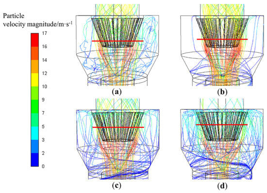
Figure 12.
Trajectories of different size particles in T-E(1-0.6): (a) d = 5 μm, (b) d = 15 μm, (c) d = 25 μm, and (d) d = 35 μm.
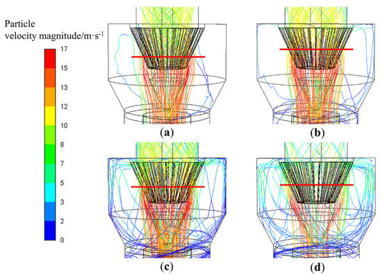
Figure 13.
Trajectories of different size particles in T-F(1-0.5): (a) d = 5 μm, (b) d = 15 μm, (c) d = 25 μm, and (d) d = 35 μm.
Simulation Results and Analysis of Multi-Particles
In order to obtain simulated Tromp curves, trajectory calculations of multi-particles were carried out for several groups of particles with different particle size. Between 1 and 89 μm, 23 groups of particles (1, 5, 9, 13, 17, 21,..., 77, 81, 85, and 89 μm) were selected. These particle trajectories were simulated by tracking 758 particles for each group. The Tromp curve is shown in Figure 14a. It is observed that the Tromp curves of T-C(1-0.8) and T-D(1-0.7) are steeper near the cut size d50 than that for T-A(1-1), T-B(1-0.9), T-E(1-0.6), and T-F(1-0.5). The Tromp curves for T-C(1-0.8) and T-D(1-0.7) are closer to the ideal classification curve. The reason for this is because the velocity distribution in the T-C(1-0.8) and T-D(1-0.7) classification areas is more uniform, and the particle concentration is more evenly distributed. The Tromp curves obtained from the simulations were used to calculate the cut size (particle size at 50% classification efficiency) and the sharpness of separation (). The results are presented in Table 5. Compared to T-A(1-1), T-C(1-0.8) and T-D(1-0.7) have a smaller cut size, in which d50 decreased from 26 μm to 22.5 μm and 22.3 μm, respectively. The grading accuracy improved from 0.42 to 0.72 and 0.71. The discrete phase simulation results verify the continuous phase results. The inverted-conical rotor cage is more suitable for the new rotor-type dynamic classifier, in which the T-C(1-0.8) and T-D(1-0.7) are the best rotor cage structures.
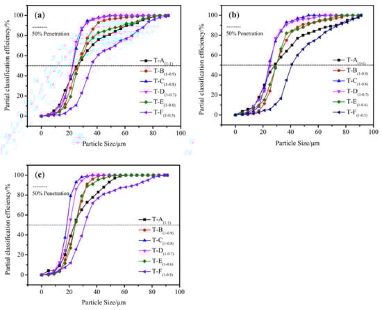
Figure 14.
Comparison of Tromp curves for six different rotor cage models: (a) 13.5 m/s–470 rpm, (b) 16 m/s–470 rpm, and (c) 13.5 m/s–670 rpm.
Table 5.
Comparison of d50 and K for the six different rotor cage models (13.5 m/s–470 rpm).
In order to investigate the effect of the operating parameters on experimental conclusions, discrete phase simulations at different air inlet velocities and rotor cage rotary speeds were conducted, including 16 m/s–470 rpm and 13.5 m/s–670 rpm. The discrete phase settings were unchanged, and trajectory tracking was performed for multi-particles with different particle sizes at different operating parameters. Figure 14b,c shows the Tromp curve of the air classifier for different operating parameters. Furthermore, by simulating the Tromp curve, the cut size and sharpness of separation were calculated for the corresponding working conditions. The results are listed in Table 6 and Table 7.
Table 6.
Comparison of d50 and K for the six different rotor cage models (16 m/s–470 rpm).
Table 7.
Comparison of d50 and K for the six different rotor cage models (13.5 m/s–670 rpm).
As can be seen from Figure 14b, the Tromp curves for T-C(1-0.8) and T-D(1-0.7) are steeper around the cut size d50 for the six different rotor cage models. The calculated classification efficiency of the T-C(1-0.8) classifier and T-D(1-0.7) classifier is better than that of the other classifier. Compared to T-A(1-1), the cut size of T-C(1-0.8) and T-D(1-0.7) is smaller, and the d50 decreased from 29.1 μm to 24.8 μm and 25.2 μm. The sharpness of separation improved from 0.47 to 0.74 and 0.75. Therefore, it can be concluded that T-C(1-0.8) and T-D(1-0.7) are still the best rotor cage structures when changing the air volume of the equipment. Compared to the original operating parameters (13.7 m/s–470 rpm), when the air inlet air volume increases, the cut size both increases and the sharpness of separation also increases for the six classifiers. This is because when the air volume increases, on the one hand, it helps to disperse the material, so that the chance of mixing the fine powder into the coarse powder is reduced; on the other hand, it also makes the radial velocity of the gas on the outer surface of the rotor increase, so that the relatively large particles can also pass through the grading surface and become fine powder. Therefore, as the air volume increases, the sharpness of separation and the cut size increases.
As can be seen from Figure 14c, among the six different models, the Tromp curves of T-C(1-0.8) and T-D(1-0.7) are steeper around the cut size d50 and are closer to the ideal classification curve. Compared to T-A(1-1), the cut size of T-C(1-0.8) and T-D(1-0.7) is smaller, and the d50 decreased from 24.1 μm to 18.9 μm and 20.1 μm. The sharpness of separation improved from 0.52 to 0.77 and 0.79. Therefore, it can be concluded that T-C(1-0.8) and T-D(1-0.7) are still the best rotor cage structures when changing the rotor cage speed. Compared with the original operating parameters (13.7 m/s–470 rpm), when the rotor cage speed increased, the cut size decreased and the sharpness of separation increased for all six models. This is because when the rotor cage speed increases, the intensity of the centrifugal force field inside the classifying chamber increases, making the fine particles also sink toward the side wall and mix into the coarse powder. Therefore, with the increase of rotor cage speed, the sharpness of separation increases and the cut size decreases.
In summary, it can be seen that when the operating parameters are changed, the cut size and sharpness of separation of the classifier will be changed. However, compared to T-A(1-1), T-B(1-0.9), T-E(1-0.6), and T-F(1-0.5), T-C(1-0.8) and T-D(1-0.7) are still the best rotor cage structures. Changes in operating parameters do not vary the internal flow characteristics of the classifier.
3.2. Influence of the Diversion Cone Structure on the Internal Flow Field in the Classifier
The diversion cone (1) guides the dusty air stream, in order to allow it to reach the vicinity of the rotor cage for classification movement, and it (2) breaks up the aggregation particles and prevents coarse particles from entering the classification chamber. The structure of the diversion cone influences the velocity distribution in the classification chamber, thereby changing the particle trajectory. The tangential velocity is mainly controlled using the rotational speed of the rotor cage. Therefore, the diversion cone structure largely influences the radial and axial velocity distribution in the classification area. This section focuses on the effect of the height and diameter of the diversion cone on the classification performance of the T-C(1-0.8) and T-D(1-0.7) classifiers.
3.2.1. Influence of Diversion Cone Height on the Flow Field
Based on the previous structure, the diversion-cone diameter to rotor-cage-chassis diameter ratio was 0.9:1.0. The diversion cone diameters for the model T-C(1:0.8) and T-D(1:0.7) were 198.0 mm and 173.3 mm. In order to study the effect of the diversion cone height on the flow field distribution, the heights were determined to be 114, 104, and 94 mm, as shown in Figure 15. Furthermore, the operating conditions are set to 13.5 m/s–470 rpm. The comparisons of radial velocity and axial velocity contours for different height diversion cones are shown in Figure 16, Figure 17, Figure 18 and Figure 19. It can be clearly observed that the radial velocity and axial velocity of the flow field is almost the same when the diversion cone diameter is constant and the height is varied. This shows that diversion cone height has almost no effect on the flow field distribution.
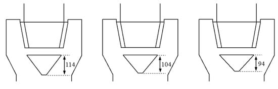
Figure 15.
Structure of the diversion cone at different heights.
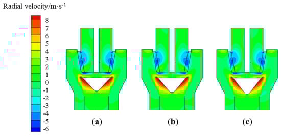
Figure 16.
Effect of the height of the diversion cone on the radial velocity (T-C(1-0.8), x = 0): (a) h = 94 mm, (b) h = 104 mm, and (c) h = 114 mm.
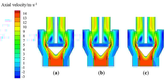
Figure 17.
Effect of the height of the diversion cone on the axial velocity (T-C(1-0.8), x = 0): (a) h = 94 mm, (b) h = 104 mm, and (c) h = 114 mm.
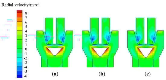
Figure 18.
Effect of the height of the diversion cone on the radial velocity (T-D(1-0.7), x = 0): (a) h = 94 mm, (b) h = 104 mm, and (c) h = 114 mm.
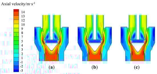
Figure 19.
Effect of the height of the diversion cone on the axial velocity (T-D(1-0.7), x = 0): (a) h = 94 mm, (b) h = 104 mm, and (c) h = 114 mm.
The discrete phase model was used to simulate the classifying motion of particles in a classifier with different diversion cone heights. Fifteen groups of particles with particle sizes of 1, 5, 9, 13, 17, 21, 25, 29, 33, 37, 41, 45, 49, 53, and 57 μm were selected. Each group tracked 758 particles in order to simulate the particle trajectory. The Tromp curve is shown in Figure 20. It can be clearly observed that the Tromp curves are almost identical, with no drastic changes in cut size or sharpness of separation. It can be concluded that influence of the classification performance of the classifier by varying the diversion cone height is not significant.
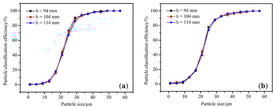
Figure 20.
Tromp curves for different height diversion cone classifiers: (a) T-C(1-0.8) and (b) T-D(1-0.7).
3.2.2. Influence of the Diversion Cone Diameter on the Flow Field
In order to determine the influence of the diversion cone diameter on the flow field, four sets of diversion cone structures were designed based on a diversion cone height of 114 mm. The diversion-cone to rotor-cage-bottom diameter ratios were 0.8:1.0, 0.9:1.0, 1.0:1.0, 1.1:1.0 (the T-C(1-0.8) classifier has diversion cone diameters of 176, 198, 220, and 242 mm, and the T-D(1-0.7) has diversion cone diameters of 154.0, 173.3, 192.5, and 211.7 mm). The structure of the diversion cone is presented in Figure 21.
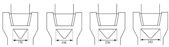
Figure 21.
Structure of the diversion cone at different diameters (T-C(1-0.8)).
The radial velocity and axial velocity contours for classifiers with different diameter diversion cones at x = 0 cross-section are presented in Figure 22, Figure 23, Figure 24 and Figure 25. As can be seen from the diagram, the flow of air can be altered by changing the diameter of the diversion cone, thereby changing the velocity distribution of the flow field. By comparing the two models, it can be seen that T-C(1-0.8) airflow distribution is similar to that for T-D(1-0.7). Therefore, T-D(1-0.7) is specifically analyzed in the present study. As shown in Figure 24a, when the diameter is 154 mm, the relatively small diameter of the diversion cone weakens the diversion cone’s action. As a result, the rotor cage chassis prevents airflow into the classification zone. The airflow that moves against the wall of the diversion cone is initially directed outwards along with the rotor cage chassis, due to the obstruction of the chassis. Then, this converges with the upward moving outer airflow. Therefore, airflow movement in the lower area of the classifying chamber is vertically upward, resulting in a relatively large axial velocity in this region. Due to the interaction between airflow, the inner airflow squeezes the outer airflow. Eventually, the airflow moves to the upper half of the classification chamber into the rotor cage. Hence, the radial velocity in the upper area of the rotor cage is relatively large, as shown in Figure 25a. The airflow carries coarse particles to the upper part of the classification chamber due to the high mass and inertia. Due to the large radial velocity and the large air drag in the upper part of the rotor cage, these coarse particles are carried through the rotor cage blades by the airflow, increasing the cut size.
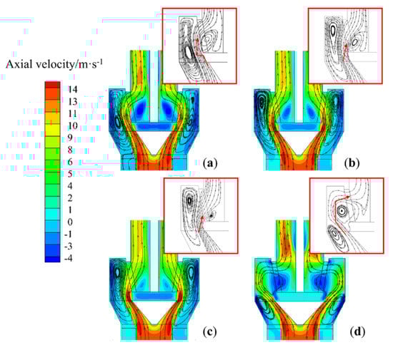
Figure 22.
Effect of the diameter of the diversion cone on the axial velocity and gas movement (T-C(1-0.8), x = 0): (a) d = 176 mm, (b) d = 198 mm, (c) d = 220 mm, and (d) d = 242 mm.
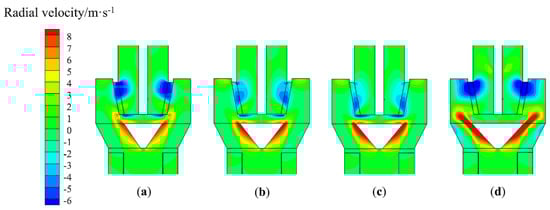
Figure 23.
Effect of the diameter of the diversion cone on the radial velocity (T-C(1-0.8), x = 0): (a) d = 176 mm, (b) d = 198 mm, (c) d = 220 mm, and (d) d = 242 mm.
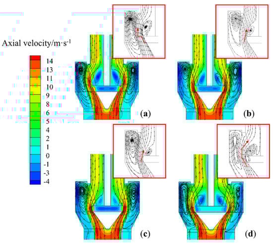
Figure 24.
Effect of the diameter of the diversion cone on the axial velocity and gas movement (T-D(1-0.7), x = 0): (a) d = 154 mm, (b) d = 173.3 mm, (c) d = 192.5 mm, and (d) d = 211.7 mm.
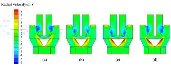
Figure 25.
Effect of the diameter of the diversion cone on the radial velocity (T-D(1-0.7), x = 0): (a) d = 154 mm, (b) d = 173.3 mm, (c) d = 192.5 mm, and (d) d = 211.7 mm.
When the diameter is 173.3 and 192.5 mm, the airflow entering the classification chamber is relatively close to the rotor cage. At the entrance to the rotor cage, the airflow incidence angle is relatively small, effectively reducing the creation of vortices at the bottom of the rotor cage. Hence, the inner airflow that moves close to the diversion cone wall can enter the cage from the bottom of the rotor cage, as shown in Figure 24b,c. This means that there will be a larger grading area, making it less likely that particles will collide with each other. The fine particles are graded in the lower area of the classification chamber. The coarse particles move to the upper area of the classification chamber and leave the classification area due to the relatively small radial velocity at the upper part of the classification chamber. Then, these hit the wall, and settle the as coarse powder.
When the diameter is 211.7 mm, the airflow into the classification chamber is far from the rotor cage. Then, a vortex forms in the lower part of the classification chamber, preventing the airflow from entering the inside of the rotor cage from the lower part of the classification chamber, as shown in Figure 24d. Due to the negative pressure in the center of the rotor cage, the airflow enters the interior of the rotor cage from the upper area of the classification chamber, resulting in a high radial velocity in the upper part of the classification chamber (Figure 25d). The concentration of particles in the upper part of the classifying chamber is relatively high, increasing the probability of particle collisions, which reduces the sharpness of separation.
In summary, it can be observed that too large or too small a diversion cone diameter leads to changes in the velocity distribution of the flow field. The flow field distribution is most reasonable when the diversion-cone diameter to rotor-cage-chassis diameter ratio is 1.0:1.0 and 0.9:1.0.
The discrete phase model was used to simulate the classifying motion of particles in classifiers with different diameter diversion cones. Nineteen groups of particles were selected between 0 and 75 μm. Each group tracked 758 particles in order to simulate the particle trajectory. The Tromp curve is shown in Figure 26. As the diversion cone diameter increased, the cut size decreased and subsequently increased. Furthermore, the sharpness of separation increased and then decreased. When the diversion-cone diameter to rotor-cage-chassis diameter ratio is 1.0:1.0 or 1.0:0.9, the cut size and sharpness of separation are approximated, and the dynamic classifier has the best classification effect.
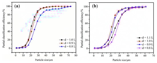
Figure 26.
Tromp curves for different diameter diversion cone classifiers: (a) T-C(1-0.8) and (b) T-D(1-0.7).
4. Industrial Application
The new rotor-type dynamic classifier has been used in the preparation of anode powder in the electrolytic aluminum industry. The process flow diagram for the grinding and classification system is presented in Figure 27a. This system is supported by a high-pressure induced draft fan, which provides power for the grinding system as a whole, and creates negative pressure in the air duct. Petroleum coke () with a particle size of 0–6 mm is uniformly fed into the air-swept ball mill via a weighing feeder. The material is continuously thrown up and sunk in the ball mill, together with the grinding media (steel balls). The fine powder suspended in the ball mill is conveyed by the wind into the new rotor-type dynamic classifier for coarse and fine separation. The fine material (d < 75 μm) enters the rotor cage and is discharged through the fine powder outlet. The coarse material (d > 75 μm) loses its momentum when it hits the cylinder wall, and drops along the wall to the bottom coarse powder discharge. Then, this returns to the air-swept ball mill for further grinding. The qualified fine powder enters the bag filter for dust–gas separation and eventually becomes the finished product.
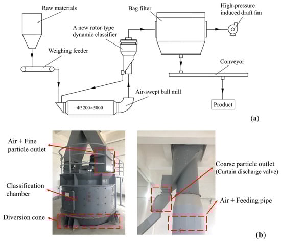
Figure 27.
(a) Process flow diagram of the grinding and classifying system and (b) photo of the industrial classifier.
According to the results of the numerical simulation, when the diameter of the top-surface to bottom-surface of the rotor cage ratio was 1.0:0.8 or 1.0:0.7, and the diversion-cone diameter to bottom-surface diameter of the rotor cage ratio was 0.9:1.0 or 1.0:1.0, the Tromp curve is closer to the ideal classification curve and the cut size is smaller and the sharpness of separation is higher (the K value is closer to 1). At this time, the dynamic classifier has better classification performance. The industrial requirements are a system output of ≥15 t/h and a finished product qualification rate (d < 75 μm) of 75 ± 5%. Then the industrial dynamic classifier was designed following a geometric scaleup according to required powder output and similar criteria. The top surface diameter of the rotor cage was 1495 mm and the chassis diameter 1050 mm; the diversion cone height was 605 mm and the diameter 945 mm. The industrial classifier is presented in Figure 27b. Through experiment on-site and testing, stable working conditions were determined: feed rate, 17 t/h; classifier inlet air velocity, 17 m/s; and rotating speed of the rotor cage 150 rpm. When the industrial classifier was running steadily, the material was picked up at the feed inlet, fine powder outlet, and coarse powder outlet at different time periods. The samples were then collected from the raw material, fine powder, and coarse powder using a sieving riffler (Quantachrome, Beach, FL, USA). The particle-size difference distribution of the samples was obtained using a Mastersizer 2000 Laser Particle Size Analyzer (Malvern Panalytical, Malvern, UK). Since the particle size distributions of the three groups of samples were not very different, only the particle size distribution of one group of samples was provided in this paper. The raw material particles are shown in Table 8. The particle size distribution of the fine and coarse powders is shown in Figure 28a.
Table 8.
Raw material particle size distribution.
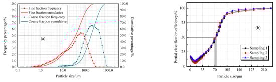
Figure 28.
(a) The particle size distribution of the coarse and fine powders and (b) Tromp curves for the industrial classifier.
As seen from Figure 28a, the volume percentage of qualifying particles (<75 μm) was around 12.88% of the collected coarse powder, indicating that only a small amount of fines are present in the coarse powder. This reduces overgrinding, lower the circulating load and reducing the process energy consumption. The product pass rate was 77.5%, meeting industrial requirements (75 ± 5%). Figure 28b shows the Tromp curve of the industrial classifier. The cut size is less than 75 μm, which guarantees the quality of the finished product. Sun [26] describes the evaluation criteria for industrial classifiers. By calculation, results indicate an industrial classifier classification efficiency of 87%, classification sharpness about 0.58, and Newton classification efficiency of 65.2%, which meet the process requirements for a specific product yield and particle size distribution. These results show that the new rotor-type dynamic classifier has excellent classification performance.
5. Conclusions
A new rotor-type dynamic classifier was designed and numerically simulated. The industrial classifier was used to classify petroleum coke and the classification performance in practical applications was obtained. The specific conclusions follow:
- The new rotor-type dynamic classifier was designed with air and material entering from the bottom. The classifier is fitted with an inverted conical rotor cage and diversion cone inside the classifier. This solved the problems of inadequate pre-dispersion and high dust concentration in the grading zone of the turbo air classifier.
- When the structural and dimensional parameters of the classifier are constant, the rotor cage structure directly influences the flow field distribution in the classifier. This influences the classification performance. The bottom of the cylindrical rotor cage generates swirls, resulting in the loss of classification function at the bottom of the rotor cage. The velocity gradient on the outer surface of the rotor cage is large and unevenly distributed. The swirl at the bottom of the inverted conical rotor cage decreases and the velocity distribution on the outer surface of the rotor cage is more uniform.
- When the top-surface to chassis-diameter ratio of the rotor cage is too large or too small, there are significant fluctuations in the tangential velocity and radial velocity. Therefore, there is an optimal for the top-surface to chassis diameter ratio of the rotor cage. This would make the standard deviations for the tangential velocity and radial velocity small, and the velocity of the flow field well-distributed.
- The height of the diversion cone has little influence on the distribution of the flow field. However, the diameter of the diversion cone has a strong influence on the radial velocity and axial velocity of the flow field.
- The industrial classifier has high classification efficiency and classification sharpness, meeting the industry requirements for classification efficiency and energy consumption.
Author Contributions
Y.F. conducted an in-depth study of existing classifiers and proposed a design concept for a new high-efficiency three separation classifier. C.C. provided resources such as experimental equipment. X.M. analyzed the classification performance of industrial-grade classifiers. F.J. was in charge of the entire research experiment and analysis of experimental results. Finally wrote and revised the manuscript. All authors have read and agreed to the published version of the manuscript.
Funding
This research was funded by the Priority Academic Program Development of Jiangsu Higher Education Institutions (PAPD).
Institutional Review Board Statement
Not applicable.
Informed Consent Statement
Not applicable.
Data Availability Statement
Not applicable.
Conflicts of Interest
The authors declare no conflict of interest.
References
- Guizani, R.; Mokni, I.; Mhiri, H.; Bournot, P. CFD modeling and analysis of the fish-hook effect on the rotor separator’s efficiency. Powder Technol. 2014, 264, 149–157. [Google Scholar] [CrossRef]
- Galletti, C.; Rum, A.; Turchi, V.; Nicolella, C. Numerical analysis of flow field and particle motion in a dynamic cyclonic selector. Adv. Powder Technol. 2020, 31, 1264–1273. [Google Scholar] [CrossRef]
- Zhao, H.; Liu, J.; Yu, Y. Effects of the impeller blade geometry on the performance of a turbo pneumatic separator. Chem. Eng. Commun. 2018, 205, 1641–1652. [Google Scholar] [CrossRef]
- Sun, J.; Li, B.; He, M. Structural analysis and improvement of the O-Sepa separator. Cement 2013, 2, 35–37. [Google Scholar]
- Lu, D.; Fan, Y.; Lu, C. Advances in research on granular air classification. China Powder Sci. Technol. 2020, 26, 11–24. [Google Scholar]
- Lu, J.; Xia, J.; He, T. Air flow field characteristics analyzing and classification process of the turbo classifier. J. Chin. Ceram. Soc. 2003, 31, 485–489. [Google Scholar]
- Shapiro, M.; Galperin, V. Air classification of solid particles: A review. Chem. Eng. Process. Process Intensif. 2005, 44, 279–285. [Google Scholar] [CrossRef]
- Gao, L.; Yu, Y.; Liu, J. Study on the cut size of a turbo air classifier. Powder Technol. 2013, 237, 520–528. [Google Scholar] [CrossRef]
- Sun, Z.; Liang, L.; Liu, C.; Yu, X.; Yang, G. Analysis of entropy generation and classification performance of turbo air classifier. Chem. Ind. Eng. Prog. 2020, 39, 3909–3915. [Google Scholar]
- Guo, L.; Liu, J.; Liu, S.; Wang, J. Velocity measurements and flow field characteristic analyses in a turbo air classifier. Powder Technol. 2007, 178, 10–16. [Google Scholar] [CrossRef]
- Xing, W.; Wang, Y.; Zhang, Y.; Yamane, Y.; Saga, M.; Lu, J.; Zhang, H.; Jin, Y. Experimental study on velocity field between two adjacent blades and gas-solid separation of a turbo air classifier. Powder Technol. 2015, 286, 240–245. [Google Scholar] [CrossRef]
- Karunakumari, L.; Eswaraiah, C.; Jayanti, S.; Narayanan, S.S. Experimental and numerical study of a rotating wheel air classifier. AIChE J. 2005, 51, 776–790. [Google Scholar] [CrossRef]
- Qiang, H.; Liu, J.; Yuan, Y. Turbo air classifier guide vane improvement and inner flow field numerical simulation. Powder Technol. 2012, 226, 10–15. [Google Scholar]
- Liu, R.; Liu, J.; Yuan, Y. Effects of axial inclined guide vanes on a turbo air classifier. Powder Technol. 2015, 280, 1–9. [Google Scholar] [CrossRef]
- Feng, Y.; Liu, J.; Liu, S. Effects of operating parameters on flow field in a turbo air classifier. Miner. Eng. 2008, 21, 598–604. [Google Scholar] [CrossRef]
- Zeng, Y.; Zhang, S.; Zhou, Y.; Li, M. Numerical Simulation of a Flow Field in a Turbo Air Classifier and Optimization of the Process Parameters. Processes 2020, 8, 237. [Google Scholar] [CrossRef]
- Guizani, R.; Mhiri, H.; Bournot, P. CFD study of the effect of rotation speed on dynamic air separator flow characteristics and pressure drop. In Proceedings of the 2014 5th International Renewable Energy Congress (IREC), Hammamet, Tunisia, 25–27 March 2014; IEEE: Piscataway, NJ, USA, 2014. [Google Scholar]
- Huang, Q.; Yu, Y.; Liu, J. Improvement on rotor cage structure of turbo air classifier and numerical simulation of inner flow field. J. Chem. Ind. Eng. 2011, 62, 1264–1268. [Google Scholar]
- Ren, W.; Liu, J.; Yu, Y. Design of a rotor cage with non-radial arc blades for turbo air classifiers. Powder Technol. 2016, 292, 46–53. [Google Scholar] [CrossRef]
- Yu, Y.; Kong, X.; Liu, J. Effect of rotor cage’s outer and inner radii on the inner flow field of the turbo air classifier. Materialwiss. Werkst. 2020, 51, 908–919. [Google Scholar] [CrossRef]
- Shukla, S.K.; Shukla, P.; Ghosh, P. Evaluation of numerical schemes using different simulation methods for the continuous phase modeling of cyclone separators. Adv. Powder Technol. 2011, 22, 209–219. [Google Scholar] [CrossRef]
- Sun, Z.; Sun, G.; Liu, J.; Yang, X. CFD simulation and optimization of the flow field in horizontal turbo air classifiers. Adv. Powder Technol. 2017, 28, 1474–1485. [Google Scholar] [CrossRef]
- Guizani, R.; Mhiri, H.; Bournot, P. Effects of the geometry of fine powder outlet on pressure drop and separation performances for dynamic separators. Powder Technol. 2017, 314, 599–607. [Google Scholar] [CrossRef]
- Morsi, S.A.; Alexander, A.J. An investigation of particle trajectories in two-phase flow systems. J. Fluid Mech. 1972, 55, 193–208. [Google Scholar] [CrossRef]
- Denmud, N.; Baite, K.; Plookphol, T.; Janudom, S. Effects of Operating Parameters on the Cut Size of Turbo Air Classifier for Particle Size Classification of SAC305 Lead-Free Solder Powder. Processes 2019, 7, 427. [Google Scholar] [CrossRef]
- Sun, Z.; Sun, G.; Peng, P.; Liu, Q.; Yu, X. A new static cyclonic classifier: Flow characteristics, performance evaluation and industrial applications. Chem. Eng. Res. Des. 2019, 45, 141–149. [Google Scholar] [CrossRef]


Publisher’s Note: MDPI stays neutral with regard to jurisdictional claims in published maps and institutional affiliations. |
© 2021 by the authors. Licensee MDPI, Basel, Switzerland. This article is an open access article distributed under the terms and conditions of the Creative Commons Attribution (CC BY) license (https://creativecommons.org/licenses/by/4.0/).