Abstract
Multipurpose stirring and blending vessels equipped with various impeller systems are indispensable in the pharmaceutical industry because of the high flexibility necessary during multiproduct manufacturing. On the other hand, process scale-up and scale-down during process development and transfer from bench or pilot to manufacturing scale, or the design of so-called scale-down models (SDMs), is a difficult task due to the geometrical differences of used vessels. The present work comprises a hybrid approach to predict mixing times from pilot to manufacturing scale for geometrical nonsimilar vessels equipped with single top, bottom or multiple eccentrically located impellers. The developed hybrid approach is based on the experimental characterization of mixing time in the dedicated equipment and evaluation of the vessel-averaged energy dissipation rate employing computational fluid dynamics (CFD) using single-phase steady-state simulations. Obtained data are consequently used to develop a correlation of mixing time as a function of vessel filling volume and vessel-averaged energy dissipation rate, which enables the prediction of mixing times in specific vessels based on the process parameters. Predicted mixing times are in good agreement with those simulated using time-dependent CFD simulations for tested operating conditions.
1. Introduction
In the field of manufacturing efficient mixing of reactants or products, blending is one of the most important challenges. For this purpose, stirred tanks are widely used because of their simple application in multipurpose facilities combined with low investment cost [1,2]. For process establishment, scale-up from bench to manufacturing scale is typically necessary. Processes are usually developed in three stages: (1) bench scale, in which screening experiments are conducted; (2) pilot plant, where optimal process parameters are defined; and (3) manufacturing scale, where the process is optimized to be economically competitive [3]. There are several approaches for scale-up, where typical scale-up follows physical characteristics such as mixing time [4], shear stress levels [5], gas–liquid and gas–solid interfaces, heat and mass transfer or geometrical similarity between reaction vessels to enable similar flow behavior in different scales. However, underlying potentially negative physical effects can balance each other, resulting in no impact on the process performance or, in the worst case, superimpose each other and lead to adverse effects such as yield reduction or the formation of unwanted byproducts.
In biopharmaceutical downstream process steps, many reactions are influenced by opposing effects, which must be assessed during process development and scale-up. It is well known that fast impeller rotational speed enables short mixing times, avoids high local concentrations of reactants and reduces aggregation of intermediates [6]. However, used reactants and produced intermediates are often prone to foaming and precipitation caused by shear forces, which results in an overall decrease in the process yield [7,8,9]. All these effects are frequently observed with new products for which there are not yet sufficient data available. In several cases, re-engineering of the process design after not meeting the quality requirements in the manufacturing scale is needed [10].
To operate economically, biopharmaceutical manufacturing utilizes the same equipment for several purposes. Universally utilizable multipurpose equipment such as stirred tanks is often used for several products for various applications within the production chain [1,2]. Due to this, the required geometrical similarity between vessels during scale-up often cannot be achieved. One- or two-impeller systems, with single or unbaffled systems, are available and used during process development. As a result, process developers are challenged to determine adequate scale-up conditions besides targeting high product quality and high step yields [10,11,12,13]. To allow comparability between scales, mixing time is considered as one of the characteristic parameters used to transfer the process in-between scales [12,13]. Apart from stirring speed, several studies have been published discussing the impact of impeller or vessel inserts on the mixing time [14,15,16,17]. These studies, as well as others [18,19,20,21,22,23,24,25,26,27,28], clearly show the benefits of computational fluid dynamics (CFD) simulations when evaluating the design of impeller geometry, including the choice of the turbulent model on the obtained results.
In this work, we performed detailed mixing time studies in stirred vessels covering nominal volumes ranging from 100 to 5000 L using experimental characterization by conductivity monitoring and CFD simulations. Due to the complexity of CFD, we also developed a simple scale-up correlation, which allows an accelerated prediction of the mixing time in multipurpose vessels equipped with single or multiple impellers filled with various volumes. The presented hybrid approach based on experimental measurements and CFD simulation is independent of geometrical similarity during scale-up and allows predicting the mixing time in the used equipment.
2. Material and Methods
2.1. Mixing Time Experiments and Experimental Data Analysis
Mixing time is defined as the time to achieve a point where the measured signal satisfies the ±5.0% criterion [29], and thus, no concentration gradient is present in the fluid. However, besides fluid properties such as density and viscosity, mixing time strongly depends on the applied stirring speed, the geometry of the impeller and the vessel and the ratio of the impeller diameter to the vessel diameter (d/D) [3,29]. The mixing time often shows variability, which is mainly caused by the used tracer and the measurement error related to the sensor setup. Therefore, trust in measured data can be achieved with an increased number of replicates.
Several methods are available to characterize the mixing process and determine the mixing time, including pH [30,31], conductivity and colorimetric [30,31] or tomographic methods [32]. Despite the simplicity of the optical method, this method can be used only in optically transparent vessels, which significantly limits its application in industrially relevant geometries. In this perspective, conductivity or pH-based methods are more suitable, even though they provide information about the local time evolution of the measured quantity. Another method to gain experimental insight into the flow pattern in the whole vessel is the application of tomography and radioactive-labeled particles [32]. This method can provide information about the tracer’s 3D distribution within the vessel over time. However, the method has several practical drawbacks when using manufacturing equipment, e.g., regarding the limited space for sensor installation, waste material treatment and strict regulations for equipment in a GMP environment.
Several tracers and sensor-based approaches are suggested in the literature [33]. Sensors with fast response times (optimally 5 times faster than measured mixing time) and measurement frequency of at least once per second are recommended [33]. When applying the approach of the global determination of mixing time, a representative sensor position must be chosen [34], and a sufficient number of replicates has to be considered [35,36]. To avoid the handling of large amounts of hazardous material, e.g., concentrated acids and bases, sodium chloride and sensitive conductivity sensors are often used in mixing time studies. Based on this analysis, the conductivity method using several sensor locations along the vessel height was used in this study.
All mixing experiments presented in this work were conducted at laboratory temperature around 22 °C using deionized water (0.9579 mPas and 997.5 kg/m3) as test fluid. A sketch of all tested equipment together with the main dimensions and sensor positions is shown in Figure 1. As a tracer solution, 0.5 M (1000, 2000 and both 5000 L vessels) or 1 M (100 and 200 L vessels) sodium chloride (Merck, Darmstadt, Germany) was used. Statistical designs considering stirring speed and liquid filling were evaluated to cover a sufficiently broad range of operating conditions. To increase the reproducibility of the tracer addition, a grid on the top of the vessel was constructed (see Figure 8). Tracer solution was always added as fast as possible (<10 s). To ensure measurement reproducibility, each measurement was performed four times. For the conduction of the mixing experiments, the volume of one tracer addition corresponded to 1.5‰ of the filling volume.
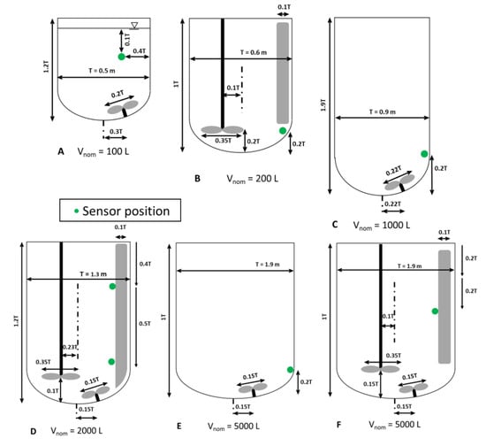
Figure 1.
Sketch of the vessels used in this work together with their main dimensions. Please note that the relative position of the baffles with respect to impellers might be different. Rotation direction is indicated as clockwise (CW) and counterclockwise (CCW) when looking from the top. The pilot-scale vessel with a working volume of 100 L was equipped with a bottom (CW) paddle impeller (A), 200 L with a top (CW) marine impeller pumping the liquid down (B), 1000 L with a bottom (CW) paddle impeller (C), 2000 L with a top (CCW) up-pumping impeller and a bottom (CW) paddle impeller (D), 5000 L vessels were equipped with a bottom (CW) paddle impeller (E) and 5000 L vessels were equipped with a combination of a top (CW) downpumping impeller and bottom (CW) paddle impeller (F). Furthermore, sensor positions are defined within the figures.
Please note that we considered only conditions where no vortex at the gas–liquid interface was formed, so the interface was approximated as flat, and no bubbles were introduced via the surface vortex into the liquid. This was particularly important for the latter CFD simulations discussed below.
The conductivity measurement was performed using an InPro 7100 (METTLER Toledo, Lutz, FL, USA) in the 100 and 200 L vessels, InPro 7108-VP (METTLER Toledo, USA) in the 1000 and 5000 L vessels with a bottom impeller and Tracksense Pro X (Ellab, Langwedel, Germany) in the 2000 and 5000 L vessels with a top and bottom impeller. The measurement accuracy of InPro7100 and InPro 718-VP was equal to 5.0%, while it was equal to 2.5% for Tracksense Pro X. The measurement interval for all vessels was selected as 1 s. The time from injection of the tracer solution until a stable conductivity signal was reached was monitored and recorded. The conductivity signal after tracer injection was considered stable when the measured conductivity shown on the transmitter device remained unchanged for at least 30 s. Subsequently, the next tracer injection was performed.
The mixing time was automatically analyzed by a Python script. Criteria for reaching homogeneity after tracer addition and, thus, the end of mixing time were set accordingly to the above-described ±5.0% signal stability. As soon as the recorded conductivity signal was in the selected range, homogeneity was assumed. For mixing experiments with 1000 and 5000 L nominal volume equipped with an InPro 718-VP probe, further data treatment using a moving average function (over 6 data points (seconds)) had to be performed, and the criterion of signal stability was set to ±10.0%. These steps had to be undertaken because of the high signal-to-noise ratio at the plateau phase between tracer additions.
2.2. Computational Fluid Dynamics (CFD)
To simulate the rotation of the impeller in all considered geometries, we utilized the sliding mesh (SM) method using ANSYS FLUENT 19.2. Each stirred vessel was divided into a rotating impeller region (or two regions in the case of two impellers) and a stationary region, where mass and momentum between rotating and stationary regions was ensured by defining the interface between these regions. The volume of rotating zones was in the range of 0.5–5%, depending on the vessel volume and type of the impeller. All fluid–solid boundaries, such as tank wall, shaft, baffles and impeller blades, were defined as nonslip boundary conditions. The gas–liquid interface was defined as a free-slip boundary condition by setting all the shear stresses equal to zero. This choice was supported by the experimental observation of a gas–liquid interface during the mixing experiment, where no extensive vortex was formed.
The realizable k-ε model (RKE) was used to model turbulence, including the flow features of strong streamline curvature, vortices and rotation [37]. The RKE comprises a new formulation for the turbulent viscosity and a new transport equation for the dissipation rate. The modeled transport equations for kinetic energy (k) and energy dissipation rate (ε) in the realizable k-ε model are
where µ is medium viscosity, µt is turbulent viscosity, and Gk and Gb is the generation of the turbulent kinetic energy due to mean velocity gradients and buoyancy, respectively.
And
where
C2, C1ε and C3ε are the model parameters [37], and values provided by Ansys Fluent were used in all simulations. σk and σε are the turbulent Prandtl numbers for k and ε. Steady-state simulations were performed initially with the moving reference frame technique, yielding a stable flow field in the vessels. From these results, transient simulations were performed with the SM technique. The mesh used in all vessels was a combination of hexahedral elements in the stationary fluid, while in the volume around the impeller, we used tetrahedral elements. The number of elements covering a range from 680,000 for the 100 L vessel to 6,900,000 for the 5000 L vessel was optimized to ensure good convergence of the solution and a reasonable time for simulations. The average aspect ratio for all meshes was around 1.5, with higher values in few computational cells. The maximum aspect ratio was always below 25. Simulations used the SIMPLE scheme to model pressure–velocity coupling and the second-order spatial discretization scheme for pressure, momentum, turbulent kinetic energy, energy dissipation rate and the tracer transport equation. The latter was modeled by the species transport model available in ANSYS FLUENT 19.2. Properties of the fluid were the same as those used during the experimental investigation considering the Newtonian behavior of the water. The solution was converged when all residuals were lower than 10−5.
The power (P) introduced in the fluid was calculated from the torque (M) acting on the impeller and shaft according to:
where N refers to impeller stirring speed in revolutions per second. In the case of multiple impellers mounted in the vessel, the power was evaluated for every impeller using Equation (4). Their sum, together with the liquid mass, was used to calculate the vessel-averaged energy dissipation rate, ⟨ε⟩. Please note that mesh quality is also supported by comparable values of ⟨ε⟩ calculated from torque and with those evaluated from the average of local ε values calculated with Equation (2). The difference was for all tested conditions always below 17%.
The impeller Reynolds number was defined as:
with D being the impeller diameter and ν corresponding to fluid kinetic viscosity. Under all tested conditions Reimpeller was above 9000, thus the conditions were considered to be turbulent. Simulation of the tracer concentration as a function of time was equivalent to the experimental procedure, including the criteria for evaluation of the mixing time considering the band of ±5.0% around the steady-state value.
3. Results and Discussion
3.1. Conductivity Probe and Logger
Figure 2 shows an example of the conducted mixing experiments in a fully filled 5000 L vessel considering both the top and bottom impeller operating. Due to the large number of conducted experiments, data analysis was performed with an automated script written in Python. The offset-corrected signal of the step input experiments shows overall good reproducibility and follows trends from the literature [30,34,35]. The step height for all replicates is comparable. Mixing times until reaching the signal stability were evaluated (see Figure 2). From the replicates, mixing time mean and standard deviation were computed and used for further data analysis and building the hybrid correlation discussed below. For all vessels, the signal stability criterion was set as ±5.0%, except for the 1000 and 5000 L vessels, which were equipped with less sensitive built-in sensors with a measurement accuracy of ±5.0% (compared to mobile sensors with a measurement accuracy of ±2.5%). The recorded signal showed stronger noise. However, as the step height remained constant (same molarity of sodium chloride was used in all manufacturing scale experiments), the signal-to-noise ratio was impaired. To allow the data analysis, signal smoothing with a moving average (as described in the Material and Methods section (Section 2)) and an acceptance criterion for mixing homogeneity set to ±10.0% was required.
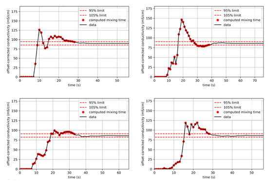
Figure 2.
Determination of mixing time in the 5000 L vessel, filled with 5000 L of deionized water. In this two-impeller system, the top impeller and the bottom impeller were operating at 100 and 50 rpm, respectively. The analyzed and offset-corrected conductivity signal from the sensor mounted on the baffle shows overall good reproducibility of the conducted step experiments. The step height for all replicates was comparable and was evaluated until signal stability of ±5.0% was reached (evaluated length of mixing time marked with red dots). The mean computed mixing time and its standard deviation were shown to be 31.75 ± 4.2 s.
3.2. Flow Pattern in Tested Vessels
The comparison of velocity vector plots normalized by the impeller tip speed in the various stirred vessels is presented in Figure 3. As can be seen, in the case of the single bottom impeller, there is a significant impact of the eccentric impeller position on the flow field in the vessel, generating liquid inflow from the upper part of the vessel into the impeller followed by liquid discharge toward the vessel periphery. In the case of two impellers, or in the case of a single marine impeller, the flow pattern is dominated by the action of the larger impeller, while the impact of the bottom impeller is less pronounced. The flow pattern is in good agreement with that generated by the axial impeller [38,39]. Despite the fact that the impellers are located close to the vessel bottom, there is visible liquid motion near the gas–liquid interphase, which documents the positive impact of the eccentric location of the impellers in all tested cases.
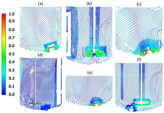
Figure 3.
Comparison of the velocity vectors normalized by the largest impeller tip speed in the various vessels studied in this work: (a) 100 L vessel with 100 L filling at 300 rpm; (b) 200 L vessel with 200 L filling at 200 rpm; (c) 1000 L vessel with 500 L filling at 150 rpm; (d) 2000 L vessel with 2000 L filling with a top impeller at 200 rpm; (e) 5000 L vessel with 3000 L filling at 150 rpm; (f) 5000 L vessel with 5000 L filling with a top impeller at 100 rpm and a bottom impeller at 50 rpm.
When looking at the contour plot of the velocity magnitude normalized by the tip speed (see Figure 4), in the case of the single bottom impeller, there is a clear stream formed from the top down to the impeller (Figure 4a,c,e), supporting the eccentric location of the impeller. In the case of the single marine impeller (Figure 4b) or its combination with the bottom radial impeller (Figure 4d,f), the velocity field is dominated by the action of the axial marine impeller. In all cases, the normalized velocity magnitude close to the impeller with the largest diameter is higher [40,41,42,43].
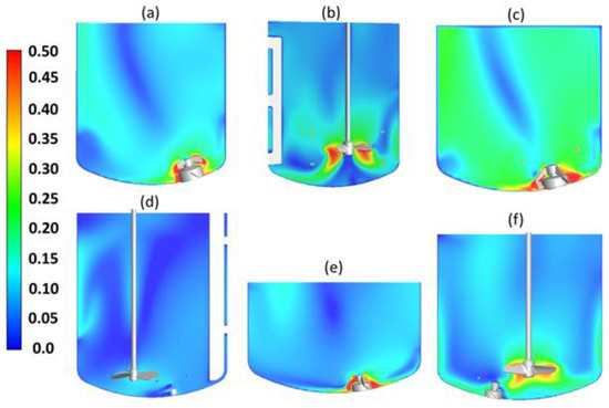
Figure 4.
Comparison of the contour plot of the velocity magnitude normalized by the largest impeller tip speed calculated for the studied vessels: (a) 100 L vessel with 100 L filling at 300 rpm; (b) 200 L vessel with 200 L filling at 200 rpm; (c) 1000 L vessel with 500 L filling at 150 rpm; (d) 2000 L vessel with 2000 L filling with a top impeller at 200 rpm; (e) 5000 L vessel with 3000 L filling at 150 rpm; (f) 5000 L vessel with 5000 L filling with a top impeller at 100 rpm and a bottom impeller at 50 rpm.
3.3. Relation of Mixing Time to Energy Dissipation Rate
As reported by Nienow [3], the mixing time in the various stirred vessels should scale with ε following the power law. Because the studied vessels have nonstandard geometry and power, the number to calculate ε is not available. We performed CFD simulations to estimate the ε for every combination of stirring speed and filling volume using a particular vessel. A comparison of the contour plots of ε is shown in Figure 5. As expected, the zone with the highest ε values is located close to the impeller blades [4,40], while the lowest values are found close to the top surface. Furthermore, it appears that vessels equipped only with a single eccentric bottom impeller exhibit larger ε heterogeneity compared to the vessels equipped with a single marine impeller or its combination with a bottom impeller. This is particularly visible for the two largest vessels with a working volume of 5000 L, where even the lower filling volume of 3000 L with the single bottom impeller is not sufficient to reduce the ε heterogeneity compared to the 5000 L vessel equipped with a combination of the marine and bottom impeller.
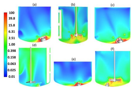
Figure 5.
Comparison of the contour plot of the turbulent energy dissipation rate normalized by the vessel-averaged values calculated for the studied vessels: (a) 100 L vessel with 100 L filling at 300 rpm; (b) 200 L vessel with 200 L filling at 200 rpm; (c) 1000 L vessel with 500 L filling at 150 rpm; (d) 2000 L vessel with 2000 L filling with a top impeller at 200 rpm; (e) 5000 L vessel with 3000 L filling at 150 rpm; (f) 5000 L vessel with 5000 L filling with a top impeller at 100 rpm and a bottom impeller at 50 rpm.
Estimated values of vessel-averaged ⟨ε⟩ were consequently used to relate the experimentally measured mixing time (see Figure 6). Together with experimental data, we also plot the theoretical scaling of the mixing time as a function of ⟨ε⟩ in a fully baffled stirred vessel with the impeller located concentrically having a height to tank diameter ratio equal to one, as reported by Nienow [3,29], indicated by a solid line with the slope equal to −1/3. As can be seen, there is a large scattering of the data points where some of them follow the theoretical scaling, while a large majority can be described by the power law with a lower slope than the theoretical one. This large variation clearly indicates that the mixing time in nonstandard partially baffled vessels with varying height to tank diameter ratios, as those presented here and commonly used in industry to perform mixing operations, cannot be described by the same relations as those obtained for impellers located in the vessel axis and equipped with baffle system. Because the main parameter, which has a strong impact on the presented scaling, is the liquid volume, we decided to include it in the mixing time relation. The idea is similar to that used by van’t Riet [44] when relating mass transfer coefficient in stirred and sparged bioreactors to the dissipated energy and superficial gas flow. In what follows we investigate the possibility to use a similar correlation also for mixing time defined as:
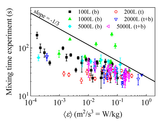
Figure 6.
Experimentally measured mixing times as a function of the turbulent energy dissipation rate for all tested vessels. A solid line indicates theoretical scaling according to Nienow ([3]) with a slope of −0.333, and a dashed line indicated the scaling of the data for the 200 L vessel. As indicated, experimental data scales with slopes are between these two limits.
By fitting the values of mixing time measured for every vessel at a given stirring speed (characterized by ⟨ε⟩ estimated from CFD) and filling volume, we found that indeed there is a good agreement between the measured values of mixing time and those obtained by Equation (6). As can be seen in Figure 7, the agreement is better for vessels up to 2000 L, while a less satisfactory agreement was found for both 5000 L vessels. The reason for this discrepancy is most probably the lack of precision of the used mixing probes combined with the reproducibility of the tracer addition. This is also reflected in the large error bars of the experimental data measured for the largest vessels, in particular for the vessel with a nominal volume of 5000 L equipped with a single bottom impeller.
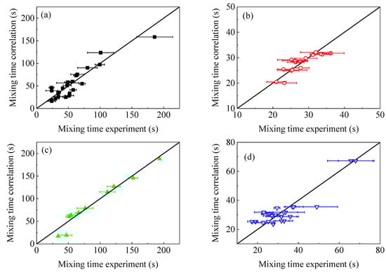
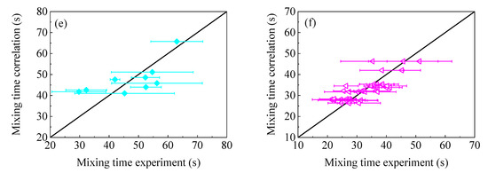
Figure 7.
Scaling of the mixing times calculated by correlation plotted as a function of the experimentally measured values. Error bars represent one standard deviation calculated from four repetitions. Vessels with nominal volume: 100 L (a); 200 L (b); 1000 L (c); 2000 L (d); 5000 L with bottom impeller (e); 5000 L with top and bottom impeller (f).
While Equation (6) represents a rather simple, albeit useful, correlation, to further extend our study, we performed a simulation of tracer mixing for selected conditions. An example of such a simulation performed in a vessel with a 5000 L nominal volume equipped with marine and bottom impeller is presented in Figure 8. As can be seen, at 10 and 20 s, there is a poorly mixed zone close to the gas–liquid interface with a higher concentration of the tracer. As we move closer to the marine impeller concentration of the tracer is more homogeneous. This is, however, not the case for the bottom impeller, where we observed a buildup of tracer concentration (see Figure 8 for 10 s).
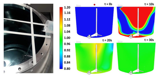
Figure 8.
Left side: Photograph of the salt solution addition in the 2000 L vessel showing the enhanced reproducibility by the introduced grid. Right side: time evolution of the added tracer solution simulated using CFD in the 5000 L vessel equipped with a top and bottom impeller operated at 100 and 50 rpm, respectively. The red dot at t = 0 s indicates the position of addition.
An example of the comparison of the tracer time evolution for all tested vessels is presented in Figure 9. Apart from the vessel with a nominal volume of 5000 L equipped with a single bottom impeller, the overall simulated tracer evolution is in good agreement with the experimental data. As discussed above, the discrepancy is due to lower sensor precision, which is indicated by the significantly slower response of the probe after tracer addition. As indicated in Figure 7, variation of the measured tracer as a function of time was lower for the smaller vessels. The presented results support the CFD approach, including turbulence model selection, used to model mixing in nonstandard vessels equipped with an eccentrically located single bottom impeller, marine impeller or combination. Here, the presented results suggest that the probes mounted in these vessels report mixing times 30 to 50% longer than real values. This relies on the measurement principle of the probes used, which presents a rather slow response, resulting in a large signal-to-noise ratio.
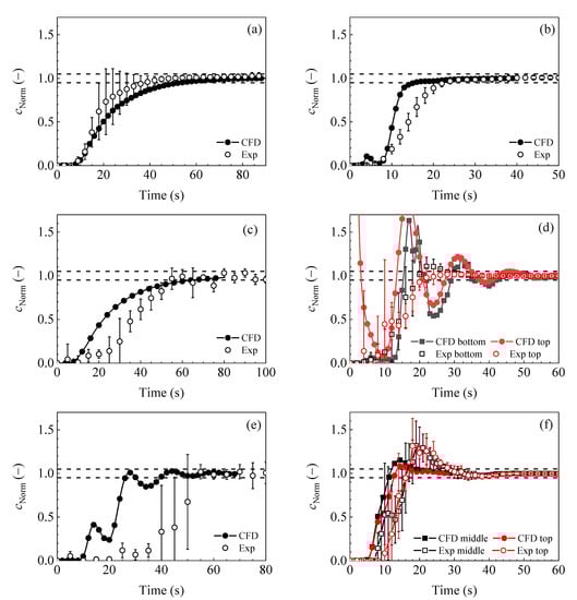
Figure 9.
Comparison of the normalized tracer concentration as a function of time for the studied vessels: (a) 100 L vessel with 100 L filling at 300 rpm; (b) 200 L vessel with 200 L filling at 200 rpm; (c) 1000 L vessel with 500 L filling at 150 rpm; (d) 2000 L vessel with 2000 L filling with a top impeller at 200 rpm; (e) 5000 L vessel with 3000 L filling at 150 rpm; (f) 5000 L vessel with 5000 L filling with a top impeller at 100 rpm and a bottom impeller at 50 rpm.
In Figure 10 is presented a comparison of the obtained values of mixing time, together with the predicted values evaluated from the correlation described by Equation (6). As evident from Figure 10, there is a significant impact of the filling volume on the values of mixing time, and thus, it has to be included in the proposed correlation (see Equation (6)). Such a correlation can be easily constructed from few experimental data points combined with rather simple CFD simulations and provides a useful tool to adjust operating conditions in the manufacturing praxis, reflecting the impact of the vessel filling volume together with energy introduced into such liquid volume.
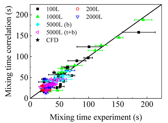
Figure 10.
Comparison of the measured mixing times and those calculated from the correction for all tested vessels. Stars indicate mixing times predicted by CFD.
4. Conclusions
In this work, we present a simple hybrid approach capable of predicting mixing time in geometrically nonsimilar vessels equipped with single or multiple eccentrically located stirrers, covering pilot up to manufacturing scales and valid for water as test media. Due to geometrical nonsimilarity, the developed hybrid approach is based on a combination of mixing time measurements using conductivity probes, while energy connected to the fluid homogenization was calculated using computational fluid dynamics (CFD). The data obtained were consequently used to develop a correlation of mixing time as a function of vessel filling volume and vessel-averaged energy dissipation rate ⟨ε⟩, which enabled the prediction of mixing times in specific vessels based on the process parameters. Furthermore, experimentally measured mixing times were compared with the simulated times using time-dependent CFD simulations, showing good agreement between CFD predictions and measured values.
Author Contributions
Conceptualization, M.C.M., C.B. and M.Š.; methodology, M.C.M., F.K., M.K., D.S., A.L. and M.B.-P.; investigation, M.C.M., F.K., M.K., D.S., A.L., M.B.-P. and M.Š.; writing—original draft preparation, all authors; visualization, M.C.M. and M.Š.; supervision, C.B. and M.Š. All authors have read and agreed to the published version of the manuscript.
Funding
This research received no external funding.
Institutional Review Board Statement
Not applicable for our work.
Informed Consent Statement
Not applicable for our work.
Data Availability Statement
Not applicable for our work.
Conflicts of Interest
The authors declare no conflict of interest.
References
- Schaber, S.D.; Gerogiorgis, D.I.; Ramachandran, R.; Evans, J.M.B.; Barton, P.I.; Trout, B.L. Economic Analysis of Integrated Continuous and Batch Pharmaceutical Manufacturing: A Case Study. Ind. Eng. Chem. Res. 2011, 50, 10083–10092. [Google Scholar] [CrossRef]
- Basu, P.; Joglekar, G.; Rai, S.; Suresh, P.; Vernon, J. Analysis of Manufacturing Costs in Pharmaceutical Companies. J. Pharm. Innov. 2008, 3, 30–40. [Google Scholar] [CrossRef]
- Nienow, A.W. Hydrodynamics of stirred bioreactors. Appl. Mech. Rev. 1998, 51, 3. [Google Scholar] [CrossRef]
- Villiger, T.K.; Neunstoecklin, B.; Karst, D.J.; Lucas, E.; Stettler, M.; Broly, H.; Morbidelli, M.; Soos, M. Experimental and CFD physical characterization of animal cell bioreactors: From micro- to production scale. Biochem. Eng. J. 2018, 131, 84–94. [Google Scholar] [CrossRef]
- Villiger, T.K.; Morbidelli, M.; Soos, M. Experimental Determination of Maximum Hydrodynamic Stress in Multiphase Flow Using a Shear Sensitive Aggregates. AIChE J. 2015, 61, 1735–1744. [Google Scholar] [CrossRef]
- Sano, Y.; Usui, H. Interrelations among mixing time, Power number and discharge flow rate number in baffled mixing vessels. J. Chem. Eng. JPN 1985, 18, 47–52. [Google Scholar] [CrossRef]
- Gikanga, B.; Chen, Y.; Stauch, O.B.; Maa, Y.F. Mixing monoclonal antibody formulations using bottom-mounted mixers: Impact of mechanism and design on drug product quality. PDA J. Pharm. Sci. Technol. 2015, 69, 284–296. [Google Scholar] [CrossRef]
- Bee, J.S.; Stevenson, J.L.; Mehta, B.; Svitel, J.; Pollastrini, J.; Platz, R.; Freund, E.; Carpenter, J.F.; Randolph, T.W. Response of a concentrated monoclonal antibody formulation to high shear. Biotechnol. Bioeng. 2009, 103, 936–943. [Google Scholar] [CrossRef] [PubMed]
- Thomas, C.R.; Geer, D. Effects of shear on proteins in solution. Biotechnol. Lett. 2011, 33, 443–456. [Google Scholar] [CrossRef]
- Yu, L.X. Pharmaceutical Quality by Design: Product and Process Development, Understanding, and Control. Pharm. Res. 2008, 25, 781–791. [Google Scholar] [CrossRef] [PubMed]
- European Medicines Agency. International Conference on Harmonisation of Technical Requirements for Registration of Pharmaceuticals for Human Use Considerations (ICH) Guideline Q8 (R2) on Pharmaceutical Development; European Medicines Agency: Amsterdam, The Netherlands, 2009. [Google Scholar]
- Chalmers, J.J. Animal Cell Culture: Effects of Agitation and Aeration on Cell Adaptation; Spier, R., Griffiths, J.B., Scragg, A.H., Eds.; Wiley: New York, NY, USA, 2000; Volume 1, pp. 41–51. [Google Scholar]
- Al-Rubeai, M. (Ed.) Animal Cell Culture; Springer International Publishing: Cham, Switzerland, 2015. [Google Scholar]
- Kumaresan, T.; Joshi, J.B. Effect of impeller design on the flow pattern and mixing in stirred tanks. Chem. Eng. J. 2006, 115, 173–193. [Google Scholar] [CrossRef]
- Mishra, S.; Kumar, V.; Sarkar, J.; Rathore, A.S. CFD based mass transfer modeling of a single use bioreactor for production of monoclonal antibody biotherapeutics. Chem. Eng. J. 2021, 412, 128592. [Google Scholar] [CrossRef]
- Jirout, T.; Jiroutová, D. Application of Theoretical and Experimental Findings for Optimization of Mixing Processes and Equipment. Processes 2020, 8, 955. [Google Scholar] [CrossRef]
- Hoseini, S.S.; Najafi, G.; Ghobadian, B.; Akbarzadeh, A.H. Impeller shape-optimization of stirred-tank reactor: CFD and fluid structure interaction analyses. Chem. Eng. J. 2021, 413, 127497. [Google Scholar] [CrossRef]
- Aubin, J.; Fletcher, D.F.; Xuereb, C. Modeling turbulent flow in stirred tanks with CFD: The influence of the modeling approach, turbulence model and numerical scheme. Exp. Therm. Fluid Sci. 2004, 28, 431–445. [Google Scholar] [CrossRef]
- Murthy, B.N.; Joshi, J.B. Assessment of standard k-epsilon, RSM and LES turbulence models in a baffled stirred vessel agitated by various impeller designs. Chem. Eng. Sci. 2008, 63, 5468–5495. [Google Scholar] [CrossRef]
- Montante, G.; Lee, K.C.; Brucato, A.; Yianneskis, M. Numerical simulations of the dependency of flow pattern on impeller clearance in stirred vessels. Chem. Eng. Sci. 2001, 56, 3751–3770. [Google Scholar] [CrossRef]
- Joshi, J.B.; Nere, N.K.; Rane, C.V.; Murthy, B.N.; Mathpati, C.S.; Patwardhan, A.W.; Ranade, V.V. CFD simulation of stirred tanks: Comparison of turbulence models. Part I Radial Flow Impellers. Can. J. Chem. Eng. 2011, 89, 23–82. [Google Scholar] [CrossRef]
- Alcamo, R.; Micale, G.; Grisafi, F.; Brucato, A.; Ciofalo, M. Large-eddy simulation of turbulent flow in an unbaffled stirred tank driven by a Rushton turbine. Chem. Eng. Sci. 2005, 60, 2303–2316. [Google Scholar] [CrossRef]
- Coroneo, M.; Montante, G.; Paglianti, A.; Magelli, F. CFD prediction of fluid flow and mixing in stirred tanks: Numerical issues about the RANS simulations. Comp. Chem. Eng. 2011, 35, 1959–1968. [Google Scholar] [CrossRef]
- Sahu, A.K.; Kumar, P.; Patwardhan, A.W.; Joshi, J.B. CFD modelling and mixing in stirred tanks. Chem. Eng. Sci. 1999, 54, 2285–2293. [Google Scholar] [CrossRef]
- Joshi, J.B.; Nere, N.K.; Rane, C.V.; Murthy, B.N.; Mathpati, C.S.; Patwardhan, A.W.; Ranade, V.V. CFD simulation of stirred tanks: Comparison of turbulence models (Part II: Axial flow impellers, multiple impellers and multiphase dispersions). Can. J. Chem. Eng. 2011, 89, 754–816. [Google Scholar] [CrossRef]
- Jaworski, Z.; Bujalski, W.; Otomo, N.; Nienow, A.W. CFD study of homogenization with dual Rushton turbines—Comparison with experimental results part I: Initial studies. Chem. Eng. Res. Des. 2000, 78, 327–333. [Google Scholar] [CrossRef]
- Bujalski, W.; Jaworski, Z.; Nienow, A.W. CFD study of homogenization with dual Rushton turbines—Comparison with experimental results part II: The multiple reference frame. Chem. Eng. Res. Des. 2002, 80, 97–104. [Google Scholar] [CrossRef]
- Zadghaffari, R.; Moghaddas, J.S.; Revstedt, J. A mixing study in a double-Rushton stirred tank. Comp. Chem. Eng. 2009, 33, 1240–1246. [Google Scholar] [CrossRef]
- Nienow, A.W. On impeller circulation and mixing effectiveness in the turbulent flow regime. Chem. Eng. Sci. 1997, 52, 2557–2565. [Google Scholar] [CrossRef]
- Rosseburg, A.; Fitschen, J.; Wutz, J.; Wucherpfennig, T.; Schlüter, M. Hydrodynamic inhomogeneities in large scale stirred tanks—Influence on mixing time. Chem. Eng. Sci. 2018, 188, 208–220. [Google Scholar] [CrossRef]
- Cabaret, F.; Bonnot, S.; Fradette, L.; Tanguy, P.A. Mixing Time Analysis Using Colorimetric Methods and Image Processing. Ind. Eng. Chem. Res. 2007, 46, 5032–5042. [Google Scholar] [CrossRef]
- Chaouki, J.; Larachi, F.; Duduković, M.P. Noninvasive Tomographic and Velocimetric Monitoring of Multiphase Flows. Ind. Eng. Chem. Res. 1997, 36, 4476–4503. [Google Scholar] [CrossRef]
- Zlokarnik, M. Stirring: Theory and Practice; Wiley-VCH: Weinheim, Germany, 2001. [Google Scholar]
- Bujalski, J.M.; Jaworski, Z.; Bujalski, W.; Nienow, A.W. The Influence of the Addition Position of a Tracer on CFD Simulated Mixing Times in a Vessel Agitated by a Rushton Turbine. Chem. Eng. Res. Des. 2002, 80, 824–831. [Google Scholar] [CrossRef]
- Oblak, B.; Babnik, S.; Erklavec-Zajec, V.; Likozar, B.; Pohar, A. Digital Twinning Process for Stirred Tank Reactors/Separation Unit Operations through Tandem Experimental/Computational Fluid Dynamics (CFD) Simulations. Processes 2020, 8, 1511. [Google Scholar] [CrossRef]
- Paul Victor, E.L.; Atiemo-Obeng, A.; Kresta, S.M. (Eds.) Handbook of Industrial Mixing; John Wiley & Sons, Inc.: Hoboken, NJ, USA, 2003. [Google Scholar]
- ANSYS FLUENT 19.2 User’s Guide; ANSYS Inc.: Canonsburg, PA, USA, 2018.
- Bugay, S.; Escudie, R.; Liné, A. Experimental analysis of hydrodynamics in axially agitated tank. AIChE J. 2002, 48, 463–475. [Google Scholar] [CrossRef]
- Delafosse, A.; Collignon, M.L.; Crine, M.; Toye, D. Estimation of the turbulent kinetic energy dissipation rate from 2D-PIV measurements in a vessel stirred by an axial Mixel TTP impeller. Chem. Eng. Sci. 2011, 66, 1728–1737. [Google Scholar] [CrossRef]
- Soos, M.; Kaufmann, R.; Winteler, R.; Kroupa, M.; Luethi, B. Determination of Maximum Turbulent Energy Dissipation Rate generated by a Rushton Impeller through Large Eddy Simulation. AIChE J. 2013, 59, 3642–3658. [Google Scholar] [CrossRef]
- Marchisio, D.L.; Soos, M.; Sefcik, J.; Morbidelli, M. Role of turbulent shear distribution in aggregation and breakage processes. AIChE J. 2006, 52, 158–173. [Google Scholar] [CrossRef]
- Marchisio, D.L.; Soos, M.; Sefcik, J.; Morbidelli, M.; Barresi, A.A.; Baldi, G. Effect of fluid dynamics on particle size distribution in particulate processes. Chem. Eng. Technol. 2006, 29, 191–199. [Google Scholar] [CrossRef]
- Ladner, T.; Odenwald, S.; Kerls, K.; Zieres, G.; Boillon, A.; Bœuf, J. CFD Supported Investigation of Shear Induced by Bottom-Mounted Magnetic Stirrer in Monoclonal Antibody Formulation. Pharm. Res. 2018, 35, 215. [Google Scholar] [CrossRef] [PubMed]
- Van’t Riet, K. Review of measuring methods and results in nonviscous gas-liquid mass transfer in stirred vessels. Ind. Eng. Chem. Process Des. Dev. 1979, 18, 357–364. [Google Scholar] [CrossRef]
Publisher’s Note: MDPI stays neutral with regard to jurisdictional claims in published maps and institutional affiliations. |
© 2021 by the authors. Licensee MDPI, Basel, Switzerland. This article is an open access article distributed under the terms and conditions of the Creative Commons Attribution (CC BY) license (https://creativecommons.org/licenses/by/4.0/).