Abstract
In this paper, a robust fuzzy controller for stochastic nonlinear systems subject to multiple performance constraints is discussed. To solve the problem of stochastic behaviors in nonlinear systems, the covariance control theory and passive control theory are applied based on the concept of energy. Additionally, the pole placement method is considered for the better transient behaviors of the system responses. However, it is known that the control inputs and maximum overshoot of the system responses may become bigger at the same time when the settling time or converge rate of the system is required to be faster. Due to this reason, the input constraint is also considered in the fuzzy controller design method to limit the value of the control gain. Moreover, an effective robust control method is applied to deal with the perturbation of the nonlinear systems. Based on the above performance constraints, the sufficient conditions can be obtained to achieve the stability in the sense of mean square and the multi-performance requirements. Finally, simulation results of the nonlinear synchronous generator system are presented to verify the feasibility and efficiency of the proposed control method.
1. Introduction
It has been witnessed that the control problem of nonlinear systems with stochastic behaviors has attracted attention greatly [1,2,3,4]. In the stability analysis and controller design method of nonlinear systems, the Takagi-Sugeno (T-S) fuzzy model can provide a powerful tool to represent these nonlinear systems by IF-THEN rules [5]. Based on the T-S fuzzy model, considerable research has been proposed to design the various control methods and obtain the distinguished results for stochastic nonlinear systems [6,7,8]. Moreover, many effective control methods have been developed based on the T-S fuzzy model and already successfully applied on the hydro-turbine, maglev vehicles, cyber-physical systems, etc. [9,10,11]. To solve the control problem of the stochastic nonlinear systems, a co-called “covariance control theory” is provided as a powerful and straightforward method [12,13]. In [12,13], it has seen that the state energy of the T-S fuzzy model, affected by the stochastic behaviors, can be analyzed by covariance matrices. Applying the upper bound matrix, these covariance matrices and the covariance matrices affected by perturbations of each fuzzy rule can all be covered under it. Then, the variance constraint is designed for the upper bound matrix in terms of root-mean-square such that all the state covariance matrices can be suppressed in the specific value. Via the applications of the upper bound state covariance matrix and variance constraint, the performance of nonlinear systems under the effect of stochastic behaviors can be guaranteed based on the T-S fuzzy model.
Based on the concept of dissipating the energy between the input and output, the passivity theory also has been proposed as a useful technique for solving the control problems of the external disturbances [14,15]. In the passivity theory, various passive properties can be obtained by selecting different power supply functions for the performance requirements. The passive control method has also been considered with the T-S fuzzy model to develop the fuzzy controller that can dissipate the energy of the external disturbance [16,17,18]. In this paper, the signal of external disturbance is considered as a stochastic behavior. Solving the control problem of stochastic external disturbance, several papers have already developed the control theory by combining the covariance control theory and passivity theory successfully [19,20]. In addition to suppressing the effect of stochastic behaviors by the variance constraint, the passivity theory is also applied to dissipate its energy. In [19,20], it can be known that the controller designed by the combined theory presents a better performance when controlling the nonlinear stochastic system than the method only applying the passivity theory. Due to this reason, the covariance control theory and passivity theory are both applied in this paper.
In many practical systems, the transient behaviors such as settling time, damping ratio, and rising time also need to be improved. Therefore, a pole placement method has been proposed to locate all the poles of the closed-loop system into a specified region, which is called “D-stable” [21]. Extending the D-stable method to the nonlinear system, many controller design methods have been developed with the T-S fuzzy model [22,23,24]. Additionally, the control problem of perturbed nonlinear systems is solved by applying the D-stable method and robust control theory [25]. In [22,23,24,25], it can be seen that the controller designed by these papers can obtain the better transient behaviors of nonlinear systems. However, it is known that the value of control gains is also much bigger when the transient behaviors such as settling time may not meet the cost-effectiveness. In the controller design of the practical systems, the control input is necessary to be constrained in order to avoid the situation that it is over the limit of the system and even cause unstableness. Due to the region, the input constraint also needs to be considered in the controller design. In [26,27], it is seen that the input constraint is combined into the fuzzy controller design based on the T-S fuzzy model and applied in practical systems successfully. Furthermore, it has to be noted that the concept of the input constraint might be opposite to the pole placement. The trade-off of each theory in the controller design method is an interesting problem that needs to be discussed. Thus, the input constraint is also applied with the D-stable method in this paper to solve the problem of huge control gains.
In this paper, a robust fuzzy controller design method is designed for the Stochastic Perturbated T-S Fuzzy Model (SPT-SFM) based nonlinear systems subject to multiple performances, including the individual state variance constraint, output variance constraint, input constraint, passive constraint, and D-stable pole constraint. Firstly, the SPT-SFM is applied to represent nonlinear systems and the fuzzy controller is designed by the Parallel Distributed Compensator (PDC) method. Then, the covariance matrices are defined for analyzing the energy of states and outputs of the closed-loop SPT-SFM. To guarantee the performances under the stochastic behavior effects, variance constraints are also designed for each covariance matrix. Moreover, the D-stable pole constraint can be constructed for the closed-loop form SPT-SFM. Considering the passivity theory and selecting the dissipate rate, the passive constraint is combined into the design method such that the SPT-SFM can dissipate the energy of stochastic behaviors. Based on the introduction of the above performance constraints, some sufficient conditions can be derived with the input constraint to satisfy the stability and multiple performance requirements. By replacing the common positive definite matrix of Lyapunov theory with the upper bound covariance matrix, the variance constraint can be applied in these sufficient conditions. Moreover, the output variance constraint can be minimized by minimizing this upper bound matrix. To eliminate the time-varying perturbed matrix of the perturbations, a robust control method is applied. Thus, the sufficient conditions can be transferred in to Linear Matrix Inequality (LMI) problems and solved by the MATLAB efficiently. Finally, a numerical example is applied to verify the proposed multiple performance constrained controller design method.
The structure of the article is as follows. In Section 2, the SPT-SFM is applied to represent the stochastic nonlinear systems with perturbations. Additionally, required definitions and useful lemmas of multiple performance constraints are given. In Section 3, the individual state variance constraint, passive constraint, and input constraint are combined into the stability analysis of the SPT-SFM and some sufficient conditions are derived. In Section 4, the D-stable pole constraint and minimized output variance constraint are applied into the proposed stability analysis with the performance constraints designed in Section 3. The sufficient conditions in LMI form are derived to achieve the stability in the sense of mean square and multiple performance requirements for the SPT-SFM. Moreover, the robust fuzzy controller can be designed via solving these conditions by MATLAB. In Section 5, the proposed design method is applied to the practical nonlinear synchronous generator system to verify the applicability and efficiency. In Section 6, some conclusions are given for this paper based on the proposed robust fuzzy controller design method and simulation results.
2. System Descriptions and Problem Statements
To develop the robust fuzzy control method for nonlinear systems subject to multiple performance constraints, some lemmas and definitions related to the design method are introduced with the T-S fuzzy model in this section. Firstly, the nonlinear systems with stochastic behaviors and perturbations can be expressed as the following SPT-SFM.
- Plant Rule i:
IF is and … and is THEN
where and denote the rules number, denotes the fuzzy sets, denotes the number of premise variables, , , and denote the state vector, control input vector, and output vector, respectively, denotes the external disturbance input vector, which is assumed as a zero-mean Gaussian white noise with the intensity . , , , , are constant matrices. Additionally, and denote the time-varying perturbations of system states and control inputs, which are expressed as and in the rest of this paper for simplicity.
Then, the overall SPT-SFM can be obtained by “blending” as follows:
where , , and are the grade of the membership of in .
It is noted that Equations (3) and (4) is the defuzzification form for the T-S fuzzy model (1)–(2). In this paper, the weighted average method is selected to construct the defuzzification process for the T-S fuzzy modeling. To design the fuzzy controller for the SPT-SFM (3)–(4), the PDC method is applied and the design process can be presented as follows. Firstly, the fuzzy controller is designed for each subsystem of the SPT-SFM (1)–(2) by the same antecedent part of fuzzy rules.
- Controller Rule i:
IF is and … and is THEN:
In the same way as the SPT-SFM (1)–(4), the overall T-S fuzzy controller can be obtained by blending each fuzzy controller of (5) as follows:
Substituting (6) into (3)–(4), the closed-loop form SPT-SFM is obtained as follows:
To analyze the state of the closed-loop SPT-SFM (7)–(8) under the effect of the stochastic behaviors, the covariance matrix can be defined based on the energy concept. Moreover, the performance requirements are usually considered in terms of the root-mean-square. Thus, the variance constraints can be designed to suppress the energy of the system states for the SPT-SFM (7)–(8), which is presented in the covariance matrix. The related definition is given as follows.
Definition 1.
Based on the concept of root-mean-square, the covariance matrix and variance constraint of system states in the SPT-SFM (7)–(8) can be defined for each fuzzy rule as follows:
wheredenotes the expectation of , the covariance matrix satisfying the condition,denotes thediagonal element of matrix, and denotes the individual state variance constraint.
In addition to the system state, the performance of the output under the effect of stochastic behaviors should also be guaranteed. Thus, the following covariance matrix and the variance constraint can be designed for the output of the SPT-SFM (7)–(8) via the similar design process of the system stated in Definition 1.
Definition 2.
Considering the outputof system (7)–(8), its covariance matrix and variance constraint can be defined as follows:
Via satisfying the variance constraint (10) and (12), the state and output performance of the SPT-SFM (7)–(8) under the effect of stochastic behaviors can be constrained in the specific value. To apply the variance constraint into the stability analysis, the corresponding Lyapunov stability conditions with the state covariance matrix (10) are presented as follows.
Lemma 1
([28]).If there exist positive definite matricessuch that the following conditions are satisfied, the SPT-SFM (7)–(8) is stable in the mean square with the variance constraint (10).
and
where.
Thus, the state performance of the SPT-SFM (7)–(8) can be guaranteed by satisfying the conditions (13)–(14), which also satisfy the variance constraint (10). Based on the concept of energy dissipating from input to the output of the system, the passive constraint also can be constructed as follows for dealing with the control problem of stochastic behaviors.
Definition 3
([29]).If there exist a positive scalarand symmetric positive definite matrix such that the following condition is satisfied, then the T-S fuzzy model (7)–(8) is strictly called input passive.
for all and .
Via satisfying the condition (15), the energy from disturbance input to the output can be dissipated by the SPT-SFM (7)–(8). Additionally, the pole placement method is applied to improve the transient responses of the system. Different from the method that assigned the system poles to the specific location, which is more difficult to achieve, an effective regional pole placement method called “D-stable” is proposed based on the LMI region in [21]. The D-stable pole placement region and the related constraints can be presented as follows.
Definition 4
([21]).In the D-stable method, the purpose is to force all the poles of a closed-loop system into a specific region. In this paper, the following circle region is selected for the pole placement region of the closed-loop systems.
whereis the center of circle andis the radius satisfying the condition.
In [22], it is noted that the pole placement method applied on a fuzzy model only needs to locate the poles of the dominant term. That is, the constraint of D-stable pole placement is only necessarily considered for the case of and not for of the SPT-SFM (7)–(8). In order to locate all the poles of each subsystem of the SPT-SFM (7)–(8) in the circle region (16), the following D-stable pole constraint is required:
Lemma 2
([30]).If there exists a common positive definite matrixsuch that the following condition is satisfied, the subsystems of the SPT-SFM (7)–(8) are called D-stable.
Then, all the poles ofcan be located in the region (16).
In the above performance constraints, it is seen that the stability conditions with state covariance matrices (13)–(14) and D-stable pole placement condition (17) consist of perturbations. Thus, an effective robust control method is applied to deal with the derivation problem of perturbations in the stability analysis and the fuzzy controller design as follows.
Lemma 3
([31]).Given real compatible dimension matrices ,, andfor any matrix ,withand , one can find two results as follows:
and
Based on the above lemmas and definitions, a robust fuzzy controller and stability analysis subject to multiple performance constraints including the state variance constraint, output variance constraint, passive constraint, D-stable pole constraint, and input constraint are developed for the SPT-SFM (7)–(8) in the following section.
3. Stability Analysis for SPT-SFM Subject to Individual State Variance Constraint, Passive Constraint, and Input Constraint
In this section, a robust fuzzy controller design method and stability analysis are proposed based on the SPT-SFM (7)–(8) subject to multiple performance constraints. For this purpose, the state variance constraint (10) and passive constraint (15) are developed with the input constraint and combined into the stability analysis. Thus, sufficient conditions can be derived in the following theorem to achieve the stability and multiple performance constraint of SPT-SFM (7)–(8) based on the Lyapunov theory.
Theorem 1.
Assuming the initial conditionof the system is known, if there exist a positive definite matrix, feedback gains, and positive scalar ,,such that the following sufficient conditions are satisfied, the closed-loop SPT-SFM (7)–(8) is stable in the mean square subject to the state variance constraint (10), passive constraint (15), and input constraint.
where,,,denotes the identity matrix for the proper dimension and * denotes the transport item in the matrices.
Proof.
Via setting and applying the Schur complement, one can obtain the following inequality if condition (20) is satisfied by Theorem 1.
To deal with the problem of perturbations, inequality (18) in Lemma 3 is applied and the following condition can also be satisfied by inequality (25) as follows:
From condition (26), one can obtain:
Then, the relationship can be obtained by subtracting (13) from (27) as follows:
Via the stability criteria designed in Theorem 1, it can be known that the SPT-SFM (7)–(8) is stable in the mean square if the sufficient conditions (20)–(24) are achieved. That is to say, the certain result can be obtained from (28) due to the system matrices of the closed-loop SPT-SFM (7)–(8) satisfying . Then, the following relationship can be obtained by condition (24) and the result .
Based on the above results, it is obvious that the upper bound state covariance matrix is applied to achieved the state variance constraint (10) by the relationship (29) in sufficient conditions (20)–(24) successfully.
Additionally, the following condition can also be obtained by applying the inequality (18) in Lemma 3 and Schur complement from condition (21).
Thus, it is obvious that the stability condition (14) can also be satisfied by condition (21) due to relationship (29). From Lemma 1 and Definition 1, the SPT-SFM (7)–(8) is said to be stable in the mean square and the state variance constraint is satisfied.
After the stability of the SPT-SFM (7)–(8) is proved, the performance requirement of the passivity which is introduced as the condition (10) should also be satisfied. To combine the condition (15) into the stability analysis and fuzzy controller design method, the performance function with Lyapunov function is designed as follows to develop the proof of the passive performance constraint:
Then, the following equation can be obtained from (31) by selecting the Lyapunov function :
Obviously, the condition for (31) is necessary to be achieved, such that the passive performance constraint (10) can be satisfied. For this purpose, the sufficient conditions (20)–(21) are also designed to satisfy the constraint (15) in addition to the stability and state variance constraint. The details of proof are given as follows.
In the above statement, it is known that the condition (26) can be satisfied by the condition (20) in Theorem 1. Then, the following condition can also be obtained by setting the positive definite matrix due to :
Moreover, the condition (30) which is satisfied by the condition (21) can be derived as follows:
Via multiplying and at the right and left-hand side of inequalities (33) and (34), it is obvious that the objective of (32), , can be achieved. Based on the results, the passive performance constraint (15) is also satisfied due to the relationship (31).
Thus, it can be said that the SPT-SFM (7)–(8) possesses the ability of dissipating the disturbance energy by satisfying the sufficient conditions (20)–(21). Note that the stability and the state variance constraint (10) can also be achieved by these conditions. Finally, the input constraint is also considered in Theorem 1 and the proof of the constraint is given as follows.
Given the assumption , the following inequality can be obtained because of the setting :
Thus, it is seen that the condition (35) can be transferred into the condition (22) by Schur complement. Then, the second condition of input constraint (23) is derived as follows. Substituting the fuzzy controller (6) into the condition , one can obtain the following inequality:
Thus,
In [12], it is known that the condition can be achieved by the conditions (13)–(14) in Lemma 1, which is the corresponding Lyapunov stability condition with state covariance matrices. The conditions (13)–(14) have already been proved in that they are satisfied by the conditions (20)–(21) of Theorem 1. Thus, the following relationship can be obtained by the fact and (35):
Then, the following relationship can be obtained from (37) and (38):
From (39), one can obtain:
It is obvious that if the condition (23) is satisfied by Theorem 1, the condition (40) can also be ensured by multiplying and applying Schur complement to (23). Therefore, it is proved that the control input constraint is enforced at all times if sufficient conditions (22)–(23) are held by Theorem 1. □
Via satisfying the sufficient conditions (20)–(24) in Theorem 1, the SPF-SFM (7)–(8) can achieve the stability in the mean square and satisfy the state variance constraint (10), passive constraint (15), and input constraint . In next section, the D-stable pole constraint (17) and output variance constraint (12), which is minimized, are considered.
4. Stability Analysis for SPT-SFM Subject to Multiple Performance Constraints
In the previous section, the stability, state variance constraint, and passive constraint are achieved for SPT-SFM (7)–(8). To improve the transient behaviors of system responses, the D-stable pole constraint (17) are combined into the stability analysis. In addition to the state variance constraint, the output variance constraint (12) is also considered to ensure the output performance under the effect of the stochastic behaviors. In the following theorem, the D-stable pole constraint (17) and output variance constraint (12) are combined with Theorem 1 to develop the stability analysis for SPT-SFM (7)–(8) satisfying the multiple performance requirements.
Theorem 2.
Assuming the initial conditionof the system is known, if there exists a positive definite matrix , feedback gains, and positive scalar ,,,such that conditions (20)–(24) and the following sufficient conditions are satisfied, the closed-loop SPT-SFM (7)–(8) is stable in the mean square subject to the state variance constraint (10), passive constraint (15), input constraint , D-stable pole constraint (17), and the output variance constraint (12) is minimized.
whereis the center andis the radius of the circle region of D-stable pole constraint.
Proof.
In Theorem 1, the conditions (20)–(24) have already been proved to satisfy the stability, state variance constraint, passive constraint, and input constraint. In the following proofs, the D-stable pole constraint (17) is proved to be satisfied and the output variance constraint (12) is proved to be minimized by minimizing the upper bound covariance matrix .
Multiplying to the right and left-hand side of the condition (41), the following condition can be obtained:
Applying Schur complement to the condition (43), one can obtain:
Then, the following condition can also be achieved by (44) and the inequality (19) in Lemma 3:
It is obvious that the D-stable pole constraint (17) can be achieved by the condition (45) and the setting . Thus, the transient behaviors of system response of the SPT-SFM (7)–(8) can be improved by the design method in Theorem 2. Next, the proof details of the minimized output variance constraint is given.
Substituting the system output (8) into the output covariance matrix (11), one can obtain:
Referring to [32], the following inequality can be obtained from (46):
Based on the fact that , the right-hand side of inequality (47) can be inferred as follows:
Then, the following inequality can be obtained due to :
Based on the results of (49), the output variance constraint (12) can be presented as follows:
It is obvious that if the upper bound state covariance matrix is minimized, then the output variance constraint (50) is minimized since the item is the given constant matrix. Therefore, the D-stable pole constraint (17) is proved to be satisfied by the condition (41) and the output variance constraint (12) is also minimized by (42) in Theorem 2. The sufficient conditions (20)–(24) are also applied to satisfy the stability, state variance constraint, passive constraint, and input constraint. It is said that the closed-loop SPT-SFM (7)–(8) can achieve stable in the mean square and is subject to multiple performance constraints by satisfying the sufficient conditions (20)–(24) and (41)–(42). □
In Theorem 2, a robust fuzzy controller is proposed for the SPT-SFM (7)–(8) to satisfy the stability, individual state variance constraint (10), passive constraint (15), input constraint, D-stable pole constraint (17), and the output variance constraint (12) is minimized. Thus, the performance of nonlinear system states and outputs under the effect of stochastic behaviors can be ensured. The effects of the stochastic behaviors can also be dissipated by the SPT-SFM (7)–(8). Additionally, the expected transient behaviors such as settling time and damping ratio can be improved by the D-stable pole method, which can specify all the poles into a given circle region.
However, the control input may become bigger, which will deteriorate the system performance and even cause unstableness, in order to achieve all the above performance requirements. To avoid the problem, the input constraints (22)–(23) are also applied to limit the magnitude of the control gains for the practical applications. In the multiple performance constrained fuzzy controller design method proposed in Theorem 2, the trade-off between the value of control gains and the better system performance also becomes an interesting issue. To verify the applicability and effectiveness of the proposed robust fuzzy controller design method, simulation results of a practical nonlinear synchronous generator system is presented in the next section.
5. Applications to a Nonlinear Synchronous Generator System
In this section, the proposed robust fuzzy controller design method is applied to a practical nonlinear synchronous generator system based on the SPT-SFM. The multiple performance requirements including the state variance constraint, passive constraint, input constraint, D-stable pole constraint, and minimized output variance constraint are also achieved. Considering a nonlinear synchronous generator system [33,34], its dynamic equations are given as follows:
where is the angular position of the rotor of the generator with respect to a synchronously rotating reference, and it is selected here to be the infinite bus, is the angular velocity of the rotor, is the electromotive force in the q-axis of the generator, is the control input, is the system output, and is external disturbance inputs.
It is noted that the disturbances of the nonlinear synchronous generator system caused by the environment can be considered such as a short circuit of induction motor, oscillations of the rotor or nonlinear friction, etc. The details of these disturbances can be referred to references [35,36] and the references cited therein. It is known that the above disturbances may affect the angular position of the rotor. Thus, the disturbance considered in this section is added into the state Equation (51).
In order to avoid the lengthy descriptions of the T-S fuzzy modeling process of the synchronous generator system, the details of the T-S fuzzy modeling process are not introduced in this paper. The details of the considered synchronous generator system and its modeling of the T-S fuzzy model can be referred to [33]. Referring to [33,34], three operating points are chosen as follows:
Based on the above operating points, the membership functions for establishing the SPT-SFM is selected as Figure 1. Then, the SPT-SFM for the synchronous generator system (51)–(54) can be constructed as follows.
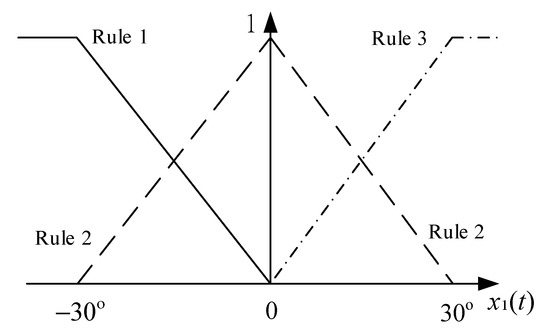
Figure 1.
The membership functions of state with three fuzzy rules.
- Plant Rule 1:
IF is about THEN
- Plant Rule 2:
IF is about THEN
- Plant Rule 3:
IF is about THEN
where the system matrices of the SPT-SFM (48) are presented as follows:
The following perturbations are also considered for system states and control inputs of the considered SPT-SFM (51)–(54):
where the perturbations structures of (62) are selected based on and with the following matrices:
According to the SPT-FSM (56)–(62), the simulation results of the practical nonlinear synchronous generator system (51)–(54) are presented in this section. To make the control process of the nonlinear synchronous generator system more clearly, the block-diagram of the proposed fuzzy control system is presented in Figure 2.
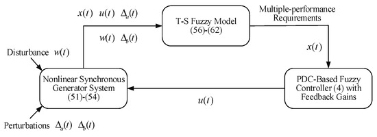
Figure 2.
Block-diagram for the nonlinear synchronous generator control system.
In this paper, the fuzzy controller design method proposed in Theorem 2 is discussed in four cases to verify the efficiency and applicability as follows.
5.1. Case 1 (Comparisons of the T-S Fuzzy Model with Selecting 3 and 4 Operating Points)
In this case, the problem of selecting operating points is discussed. Three operating points are chosen as (55) for constructing the SPT-SFM (56)–(62) with three fuzzy rules. To present the applicability of the SPT-SFM (56)–(62), the simulation results compared with the T-S fuzzy model with four fuzzy rules are presented as follows. Firstly, let us choose four operating points as follows:
In order to make the comparison results more precise, the perturbations are not considered in this simulation case. Based on the operating points of (63), the membership functions are presented in Figure 3.
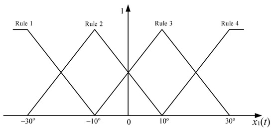
Figure 3.
The membership functions of state with three fuzzy rules.
Then, the SPT-SFM for the nonlinear synchronous generator system (46) with four fuzzy rules can be constructed as follows.
- Plant Rule 1:
IF is about THEN
- Plant Rule 2:
IF is about THEN
- Plant Rule 3:
IF is about THEN
- Plant Rule 4:
IF is about THEN
where the system matrices are given as follows:
Considering multiple constraints, the state variance constraints , input constraint , passive constraint , , and D-stable pole constraint are selected for this simulation case. Then, the following control gains can be obtained by solving the sufficient conditions (20)–(24) and (41)–(42) for the SPT-SFM (56)–(61) and (64)–(71), respectively.
For the SPT-SFM (56)–(61), the feedback gains can be solved as follows:
For the SPT-SFM (64)–(71), the feedback gains can be solved as follows:
Applying the feedback gains (72) and (73) to the fuzzy controller (6) and selecting the initial conditions , the system responses of nonlinear system (51)–(54) are presented in Figure 4, Figure 5, Figure 6 and Figure 7.
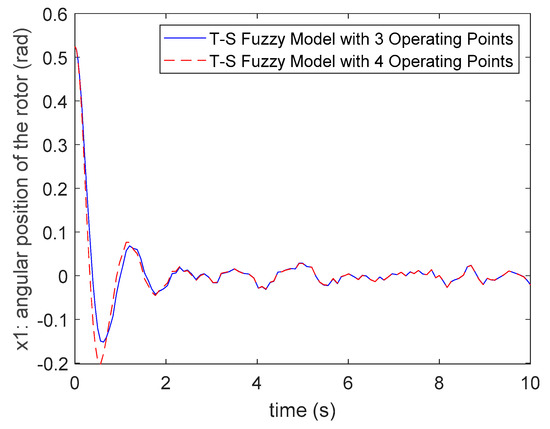
Figure 4.
The comparisons of state . responses for Case 1.
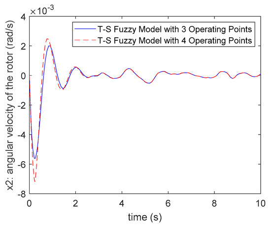
Figure 5.
The comparisons of state . responses for Case 1.
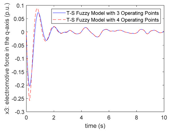
Figure 6.
The comparisons of state . responses for Case 1.
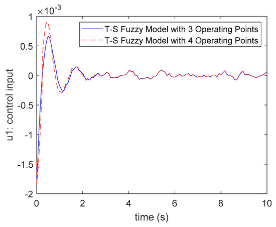
Figure 7.
The comparisons of control input . responses for Case 1.
Comparing (72) and (73), it is obvious that the control gains of the three fuzzy rules case and four fuzzy rules case are similar. In addition, the responses of system states and inputs are also similar for these two cases. Hence, it can be found that there is not much difference in system responses when one chooses three operating points or four operating points for modeling the T-S fuzzy model. In the T-S fuzzy modeling method for nonlinear systems, the operating points or fuzzy rules of the fuzzy model are selected as more as possible to represent the original nonlinear system more precisely. However, it will also cause the difficulties of the stability analysis and fuzzy controller design for the system. Therefore, it is sufficient to select an appropriate number of operating points and fuzzy rules for a nonlinear system. For the nonlinear synchronous generator system (46), it can be found that the three fuzzy rules SPT-SFM (56)–(62) are sufficient to deal with the proposed multiple performance constraints control problem.
5.2. Case 2 (Comparisons of Different State Variance Constraints)
Based on the results of Case 1, the SPT-SFM (56)–(62) is considered for the following control case. In this case, the simulation results for different state variance constraints are presented. To present the comparison results more clearly, the D-stable pole constraint and input constraint are not considered in this case. In this case, the initial condition , the variance of disturbance , and passive constraint , are selected. Moreover, the disturbance matrices are selected as to amplify the influence of disturbance on state variances. By solving the sufficient conditions (20)–(24) and (41)–(42), the compared results are shown in Table 1.

Table 1.
Comparison results for different state variance constraints in Case 2.
From Table 1, it is obvious that if the smaller state variance constraints need to be achieved, the feedback gains must become bigger. That is, the control force needs to be stronger to achieve the more rigorous performance requirements. Moreover, the variance values of the simulation results can achieve smaller values if the smaller variance constraints are assigned. Thus, the effect of the state variance constraint in the proposed design method can be concluded such that if the smaller variance constraint is assigned, then the smaller variance values of system states can be achieved. However, the corresponding control inputs must also become bigger to achieve the smaller variance constraints.
5.3. Case 3 (Comparisons of Different D-Stable Pole Constraints)
In this case, the different circle regions of the D-stable pole constraint for the proposed design method are discussed. Based on the SPT-SFM (56)–(62), the simulation results can be presented as follows. By setting the passive constraint , , state variance constraint, , , , and input constraint , the following feedback gains can be obtained by solving the sufficient conditions (20)–(24) and (41)–(42) with three different circle regions.
For circle region :
For circle region :
For circle region :
Using the control gains of (74)–(76), the closed-loop poles can be presented for each subsystem of SPT-SFM (56)–(62) as follows.
For circle region :
For circle region :
For circle region :
From the results of (77)–(79), it can be seen that all the poles of each subsystem can be located in the assigned circle region. The pole locations of (77)–(79) and the corresponding circle regions are presented in Figure 8. Applying the control gains (74)–(76) to the fuzzy controller (6), the system responses of the nonlinear synchronous generator system can be presented in Figure 9, Figure 10, Figure 11 and Figure 12. From Figure 8, it can be found that when we choose the bigger circle region, the dominant pole will move more to the left. That is, if the center of circle region of the proposed fuzzy controller design method is assigned as more negative, then the poles of the closed-loop system will be placed to the more negative location on the complex-plane. In this case, a faster converge rate of the state responses will be obtained. It can be verified from the state responses shown in Figure 9, Figure 10 and Figure 11.
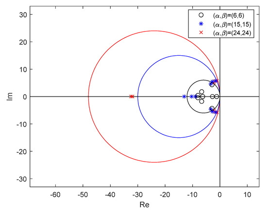
Figure 8.
The comparisons of pole locations with different circle regions.
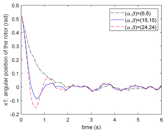
Figure 9.
The comparisons of state . responses for different circle regions.
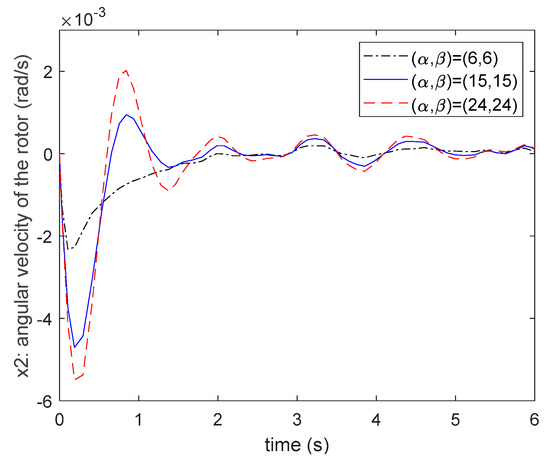
Figure 10.
The comparisons of state . responses for different circle regions.
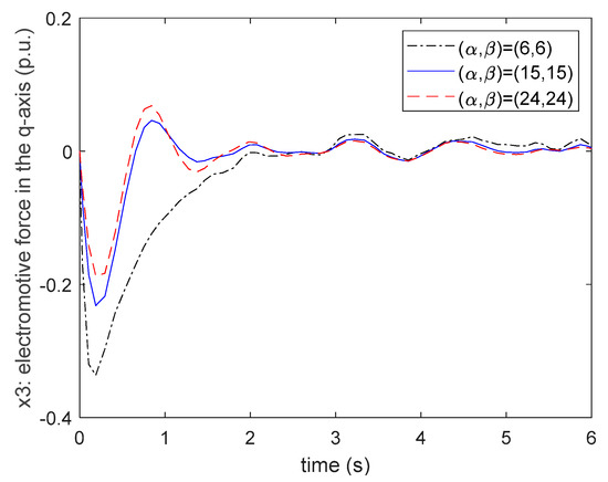
Figure 11.
The comparisons of state . responses for different circle regions.
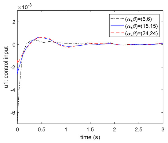
Figure 12.
The comparisons of control input . responses for different circle regions.
From Figure 9, Figure 10, Figure 11 and Figure 12, one can find that the responses obtained by the region and can achieve a faster converge rate than the responses obtained by . Moreover, the value of the control input obtained by is bigger than others. Thus, the circle region is not a better choice for the designers for considering the D-stable pole constraint. Next, let us compare the responses obtained by and from Figure 9, Figure 10 and Figure 11. It can be found that the oscillation and the maximum overshoot of the responses obtained by are bigger than the responses obtained by . Moreover, the control inputs shown in Figure 12 are very close for both cases. Based on the above results, it is obvious that the region is the best choice for obtaining the faster settling time and smaller maximum overshoot.
5.4. Case 4 (Compare the Proposed Fuzzy Control Method with the Previous Design Method)
Based on the results of Case 1, the SPT-SFM (56)–(62) is a suitable fuzzy model to represent the nonlinear synchronous generator system (51)–(54). From Case 2, it is verified that setting a smaller state variance constraint will suppress the effect of disturbances. However, it will also increase the control gains at the same time. From Case 3, it is known that the circle region is the most proper choice for the D-stable pole constraint that can obtain a better transient response for the system (51)–(54). Thus, the above performance constraints are chosen to compare the proposed fuzzy control method with the design method developed in [28]. In the fuzzy control method of [28], the performance requirements including the state variance constraint, output variance constraint, and D-stable pole constraint were considered for the nonlinear systems based on SPT-SFM. To achieve the better performance and feasibility of the practical applications, the passive constraint is considered in this paper to dissipate the effect of disturbances. Moreover, the input constraint is also considered in this paper to ensure that the control input will not exceed a reasonable range of the system. The details of the performance constraints considered in the proposed design method and the design method of [28] are presented in Table 2.
Table 2.
Selected multiple performance constraints.
From Table 2, the individual state variance constraint, D-stable pole constraint, passive constraint, and input constraint are considered in this paper. The purposes of each constraint are introduced as follows. Firstly, the state variance constraints , , are selected as different values for each method. Via the given specific value of variance constraint, the state energy of system (51)–(54) under the effect of disturbance can be suppressed in the value by the relationship (10) and (29). Secondly, considering the D-stable pole constraint with the circle region , all closed-loop poles of each subsystem (56)–(62) can be located in the specific circle region with center and radius on the complex-plane. To get a better settling time and smaller maximum overshoot, the circle region is selected for both design methods for obtaining transient responses of the system (51)–(54). Thirdly, via satisfying the passive constraint (10), the synchronous generator system (51)–(54) can dissipate the energy of the disturbance. The details of the passive constraint can be referred to [29]. Moreover, the dissipate ability of the system are related to the dissipate rate and dissipate matrix . Finally, the input constraint is applied to limit the norm of control input in a specific value. The energy of the control input of system (51)–(54) can be constrained under the given value to obtain smaller control inputs. Thus, the cost-effective controller can be obtained for the system (51)–(54) and it also can ensure the control signals under an assigned limit.
Considering the performance constraints in Table 2 and solving the sufficient conditions (20)–(24) and (41)–(42) in Theorem 2 for the SPT-FSM (56)–(62), the following results of the upper bound covariance matrix and feedback gains can be obtained:
Additionally, the corresponding upper bound covariance matrix and feedback gains obtained by the design method of [28] are presented as follows:
Using the fuzzy control gains of (82), the closed-loop poles of each subsystem of the SPT-SFM (56)–(62) can be shown as follows:
Similarly, the closed-loop poles of each subsystem obtained by the fuzzy control gains (83) of the design method [28] with the same D-stable pole constraint are also presented as follows:
It is obvious that all the poles of both (84) and (85) are located in the given circle region . Applying the control gains of (81) and (83) to the fuzzy controller (6) for the SPT-SFM (56)–(62) and giving the initial condition , the responses of the system’s states and control inputs are presented in Figure 13, Figure 14, Figure 15 and Figure 16. From the responses shown in Figure 13, Figure 14 and Figure 15, the individual state variance values controlled by the proposed design method and the design method of [28] are compared as follows.
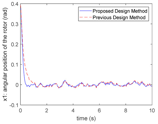
Figure 13.
The comparison of state . response with the method in [28].
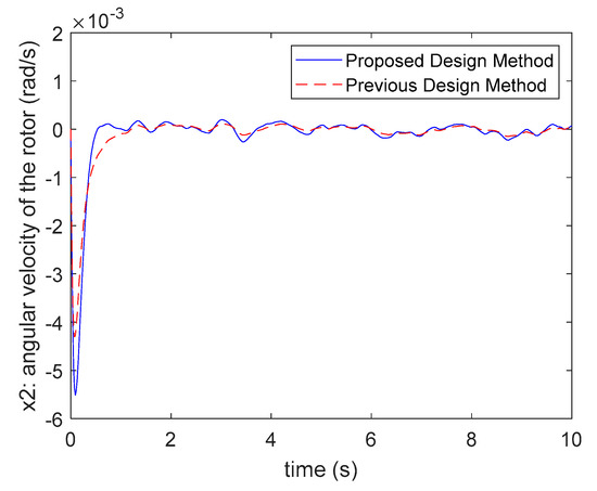
Figure 14.
The comparison of state . response with the method in [28].
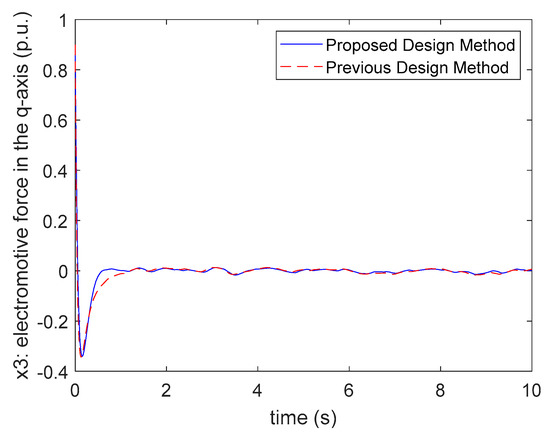
Figure 15.
The comparison of state . response with the method in [28].
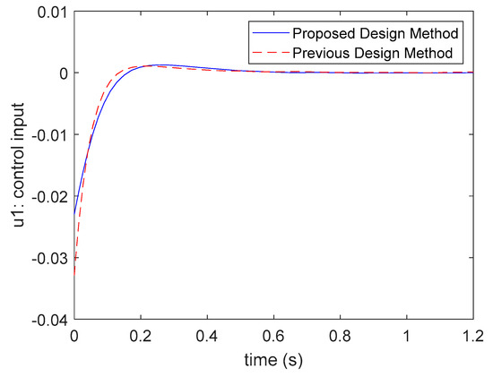
Figure 16.
The comparison of control input . response with the method in [28].
The state variance values controlled by the proposed design method are shown as follows:
Similarly, the state variance values controlled by the design method of [28] are shown as follows:
According to the state variance constraints assigned in Table 2, the state variance values of each state shown in (86)–(87) all satisfy the given variance constraints for both design methods. From Figure 13, Figure 14 and Figure 15, it is seen that both design methods can suppress the effect of disturbance behaviors via considering the state variance constraints. However, the proposed design method has a relatively small settling time and converge rate. Hence, a better transient behavior can be obtained by the proposed design method. From Figure 16, it can be found that the control inputs obtained by the proposed design method can satisfy the input constraint , but the design method of [28] cannot satisfy it. That is, the proposed design method is able to achieve better responses using fewer costs of the control inputs by considering the input constraints in the design process.
Moreover, the passive constraint is considered in the proposed fuzzy control method with the state variance constraint to guarantee the system performance under the effects of disturbance behaviors. The passive constraint (15) is verified based on the simulation results as follows:
From (88), one can find that the passive constraint (15) is satisfied for the SPT-SFM (56)–(62) controlled by the proposed fuzzy controller design method. From Table 2 and Figure 13, Figure 14, Figure 15 and Figure 16, it is seen that although the individual state variance constraint of the design method [28] can be chosen in the much smaller value, the same ability of resisting the effect of disturbance behaviors can also be achieved by the proposed fuzzy control method via combining the variance constraint and passive constraint. Thus, it can be concluded that the proposed fuzzy controller design method provided a better choice for controlling nonlinear systems to achieve the stability subject to multiple performance constraints by applying the cost-effective fuzzy controllers.
6. Conclusions
Based on the SPT-SFM, a stability analysis and robust fuzzy controller design method subject to multiple performance constraints are proposed for the stochastic nonlinear systems with perturbations in this paper. The state variance constraint and minimized output variance constraint are applied to suppress the energy of the system state and output under the stochastic behaviors effect. Moreover, the passive constraint is combined into the design method to dissipate the energy of stochastic behaviors. Furthermore, to improve the transient behaviors of system response, the D-stable pole placement constraint is considered. It is expected that the control input may become bigger even over the limit of the system since all the above performance constraints need to be ensured. Due to this reason, the input constraint is also applied in the robust fuzzy controller design method to guarantee the control input in the specific value. From the simulation results of the synchronous generator system, it is known that the better system responses can be obtained via using the smaller control force by the proposed robust fuzzy controller design method. Therefore, this paper provides a more efficient controller design method for stochastic perturbed nonlinear systems to achieve the multiple performance requirements.
Author Contributions
Conceptualization, H.Q. and W.-J.C.; methodology, H.Q. and W.-J.C.; software, Y.-H.L. and Y.-W.L.; validation, W.-J.C.; investigation, Y.-H.L. and Y.-W.L.; writing—original draft preparation, H.Q. and Y.-H.L.; writing—review and editing, W.-J.C., H.Q. and Y.-H.L. All authors have read and agreed to the published version of the manuscript.
Funding
This research was funded by Natural Science Foundation of the Jiangsu Higher Education Institutions of China, grant number 17KJD413001.
Acknowledgments
The authors would like to express their sincere gratitude to the anonymous reviewers who gave us many constructive comments and suggestions. This work was sponsored by the Natural Science Foundation of the Jiangsu Higher Education Institutions of China (grant number 17KJD413001).
Conflicts of Interest
The authors declare no conflict of interest.
References
- Li, L.; Zhang, Q.; Zhu, B. Fuzzy stochastic optimal guaranteed cost control of bio-economic singular Markovian jump systems. IEEE Trans. Cybern. 2015, 45, 2512–2521. [Google Scholar] [CrossRef]
- Wang, Y.; Xia, Y.; Li, H.; Zhou, P. A new integral sliding mode design method for nonlinear stochastic systems. Automatica 2018, 90, 304–309. [Google Scholar] [CrossRef]
- Min, H.; Xu, S.; Zhang, B.; Ma, Q. Output-feedback control for stochastic nonlinear systems subject to input saturation and time-varying delay. IEEE Trans. Autom. Control 2019, 64, 359–364. [Google Scholar] [CrossRef]
- Liu, W.; Lu, J.; Xu, S.; Li, Y.; Zhang, Z. Sampled-data controller design and stability analysis for nonlinear systems with input saturation and disturbances. Appl. Math. Comput. 2019, 360, 14–27. [Google Scholar] [CrossRef]
- Wang, H.O.; Tanaka, K.; Griffin, M.F. An approach to fuzzy control of nonlinear systems: Stability and design issues. IEEE Trans. Fuzzy Syst. 1996, 4, 14–23. [Google Scholar] [CrossRef]
- Sui, S.; Li, Y.; Tong, S. Adaptive fuzzy control design and applications of uncertain stochastic nonlinear systems with input saturation. Neurocomputing 2015, 156, 42–51. [Google Scholar] [CrossRef]
- Wei, Y.; Qiu, J.; Lam, H.K.; Wu, L. Approaches to T-S fuzzy-affine-model-based reliable output feedback control for nonlinear Itô stochastic systems. IEEE Trans. Fuzzy Syst. 2017, 25, 569–583. [Google Scholar] [CrossRef]
- Wang, Y.; Shen, H.; Karimi, H.R.; Duan, D. Dissipativity-based fuzzy integral sliding mode control of continuous-time T-S fuzzy systems. IEEE Trans. Fuzzy Syst. 2018, 26, 1164–1176. [Google Scholar] [CrossRef]
- Wang, B.; Xue, J.; Wu, F.; Zhu, D. Robust Takagi-Sugeno fuzzy control for fractional order hydro-turbine governing system. ISA Trans. 2016, 65, 72–80. [Google Scholar] [CrossRef]
- Sun, Y.G.; Xu, J.Q.; Chen, C.; Lin, G.B. Fuzzy H∞ robust control for magnetic levitation system of maglev vehicles based on T-S fuzzy model: Design and experiments. J. Intell. Fuzzy Syst. 2019, 36, 911–922. [Google Scholar] [CrossRef]
- Zhang, D.; Song, H.; Yu, L. Robust fuzzy-model-based filtering for nonlinear cyber-physical systems with multiple stochastic incomplete measurements. IEEE Trans. Syst. Man Cybern. Syst. 2017, 47, 1826–1838. [Google Scholar] [CrossRef]
- Chang, W.J.; Wu, S.M. Continuous fuzzy controller design subject to minimizing control input energy with output variance constraints. Eur. J. Control 2005, 11, 377–387. [Google Scholar] [CrossRef]
- Chang, W.J.; Wu, S.M. Fuzzy control with input energy and state variance constraints for perturbed ship steering systems. Int. J. Comput. Appl. Technol. 2006, 27, 133–143. [Google Scholar] [CrossRef]
- Xie, L.; Fu, M.; Li, H. Passivity analysis and passification for uncertain signal processing systems. IEEE Trans. Signal Process. 1998, 46, 2394–22403. [Google Scholar]
- Uang, H.J. On the dissipativity of nonlinear systems: Fuzzy control approach. Fuzzy Sets Syst. 2005, 156, 185–207. [Google Scholar] [CrossRef]
- Su, L.; Ye, D. Mixed H∞ and passive event-triggered reliable control for T-S fuzzy Markov jump systems. Neurocomputing 2018, 281, 96–105. [Google Scholar] [CrossRef]
- Yin, X.; Song, X.; Wang, M. Passive fuzzy control design for a class of nonlinear distributed parameter systems with time-varying delay. Int. J. Control Autom. Syst. 2020, 18, 911–921. [Google Scholar] [CrossRef]
- Pang, B.; Zhang, Q. Observer-based passive control for polynomial fuzzy singular systems with time-delay via sliding mode control. Nonlinear Anal. Hybrid Syst. 2020, 37, 100909. [Google Scholar] [CrossRef]
- Chang, W.J.; Huang, B.J. Robust fuzzy control subject to state variance and passivity constraints for perturbed nonlinear systems with multiplicative noises. ISA Trans. 2014, 53, 1787–1795. [Google Scholar] [CrossRef]
- Chang, W.J.; Chen, P.H.; Ku, C.C. Mixed sliding mode fuzzy control for discrete-time non-linear stochastic systems subject to variance and passivity constraints. IET Control Theory Appl. 2015, 9, 2369–2376. [Google Scholar] [CrossRef]
- Chilali, M.; Gahinet, P. H∞ design with pole placement constraints: An LMI approach. IEEE Trans. Autom. Control 1996, 41, 358–367. [Google Scholar] [CrossRef]
- Hong, S.K.; Nam, Y. Stable fuzzy control system design with pole-placement constraint: LMI approach. Comput. Ind. 2003, 51, 1–11. [Google Scholar] [CrossRef]
- Cherifi, A.; Guelton, K.; Arcese, L.; Leite, V.J.S. Global non-quadratic D-stabilization of Takagi-Sugeno systems with piecewise continuous membership functions. Appl. Math. Comput. 2019, 351, 23–36. [Google Scholar] [CrossRef]
- Mardani, M.M.; Vafamand, N.; Khooban, M.H.; Dragičević, T.; Blaabjerg, F. Design of quadratic D-stable fuzzy controller for microgrids with multiple CPLs. IEEE Trans. Ind. Electron. 2019, 66, 4805–4812. [Google Scholar] [CrossRef]
- Cherifi, A.; Guelton, K.; Arcese, L. Uncertain T-S model-based robust controller design with D-stability constraints- A simulation study of quadrotor attitude stabilization. Eng. Appl. Artif. Intell. 2018, 67, 419–429. [Google Scholar] [CrossRef]
- Saifia, D.; Chadli, M.; Karimi, H.R.; Labiod, S. Fuzzy control for electric power steering system with assist motor current input constraints. J. Frankl. Inst. 2015, 351, 562–576. [Google Scholar] [CrossRef]
- Kong, L.; Yuan, J. Disturbance-observer-based fuzzy model predictive control for nonlinear processes with disturbances and input constraints. ISA Trans. 2019, 90, 74–88. [Google Scholar] [CrossRef]
- Chang, W.J.; Lin, Y.H.; Du, J.; Chang, C.M. Fuzzy control with pole assignment and variance constraints for continuous-time perturbed Takagi-Sugeno fuzzy models: Application to ship steering systems. Int. J. Control Autom. Syst. 2019, 17, 2677–2692. [Google Scholar] [CrossRef]
- Ku, C.C.; Huang, P.H.; Chang, W.J. Passive fuzzy controller design for nonlinear systems with multiplicative noises. J. Frankl. Inst. 2010, 347, 732–750. [Google Scholar] [CrossRef]
- Garcia, G.; Bernussou, J. Pole assignment for uncertain systems in a specified disk by state feedback. IEEE Trans. Autom. Control 1995, 40, 184–190. [Google Scholar] [CrossRef]
- Chang, W.J.; Ku, C.C.; Huang, P.H. Robust fuzzy control for uncertain stochastic time-delay Takagi-Sugeno fuzzy models for achieving passivity. Fuzzy Sets Syst. 2010, 161, 2012–2032. [Google Scholar] [CrossRef]
- Jadbabaie, A.; Jamshidi, M.; Titli, A. Guaranteed-cost design of continuous-time Takagi-Sugeno fuzzy controllers via linear matrix inequalities. Proc. IEEE Int. Conf. Fuzzy Syst. 1998, 1, 268–273. [Google Scholar]
- Zheng, F.; Wang, Q.G.; Lee, T.H.; Huang, X. Robust PI controller design for nonlinear systems via fuzzy modeling method. IEEE Trans. Syst. Man Cybern. 2001, 31, 666–675. [Google Scholar] [CrossRef]
- Chang, W.J.; Huang, B.J. Passive fuzzy controller design with variance constraint for nonlinear synchronous generator systems. In Proceedings of the IEEE 10th International Conference on Power Electronics and Drive Systems, Kitakyushu, Japan, 22–25 April 2013; pp. 1251–1256. [Google Scholar]
- Bergen, A.R. Power System Analysis; Prentice-Hall: Englewood Cliffs, NJ, USA, 1986. [Google Scholar]
- Su, Y.X.; Zheng, C.H.; Duan, B.Y. Automatic disturbances rejection controller for precise motion control of permanent-magnet synchronous motors. IEEE Trans. Ind. Electron. 2005, 52, 814–823. [Google Scholar] [CrossRef]
Publisher’s Note: MDPI stays neutral with regard to jurisdictional claims in published maps and institutional affiliations. |
© 2021 by the authors. Licensee MDPI, Basel, Switzerland. This article is an open access article distributed under the terms and conditions of the Creative Commons Attribution (CC BY) license (https://creativecommons.org/licenses/by/4.0/).