1. Introduction
The fuzzy set provides a concept differing from the crisp set for discussing the problems of economics, management, and control. During fuzzification, the states in the nonlinearity are usually premise variables. Moreover, the linear systems and the membership function can be determined via the chosen equilibrium points to build the T–S fuzzy system. Furthermore, the center of gravity method [
1] is a common defuzzification technique method and is used to convert the fuzzified output into a single crisp value with respect to a fuzzy set. Referring to [
2], the fuzzy set was applied to formulate the mathematical model of optimization of sustainable waste management. In the past decades, the Takagi–Sugeno (T–S) fuzzy system has been widely used by blending some subsystems and the specific membership function to represent nonlinear systems. In the literature [
3,
4,
5,
6,
7,
8,
9,
10,
11,
12,
13], several results for the control problem of nonlinear systems have been already dealt with using linear control theories through the T–S fuzzy system. T–S fuzzy systems have also been investigated for their use in stability issues of practical systems such as turbocharged gasoline engines [
9], flexible wings [
10], and vessel dynamic positioning [
11]. To develop the controller design method for T–S fuzzy systems, the parallel distributed compensation (PDC) concept was first proposed [
12]. Similar to the structure of the T–S fuzzy system, the PDC technique involves setting up a unique subcontroller for each linear subsystem and blending them with a specific membership function. Referring to the literature [
5,
6,
9,
10,
11,
12], the PDC concept has been applied successfully and widely to design corresponding fuzzy controllers. Most of the existing PDC-based controller design methods [
5,
6,
9,
10,
11,
12] were proposed using a state-feedback scheme. The control problems of nonlinear systems with unmeasurable states were discussed by designing observer-based controllers [
13,
14], a dynamic output controller [
15], and a static output controller [
16]. It is well-known that the static output feedback control scheme [
16] is a reasonable and easy method for solving the stabilization issue of systems with unmeasured states. Because of this, the control problem of the output feedback technique, which uses measurable states as feedback signals, becomes a worthy issue for discussion and investigation regarding T–S fuzzy systems.
The output control problems of polynomial systems, such as the T–S fuzzy system [
17,
18] and the linear parameter varying system [
19], usually become complex and difficult according to the number of sufficient conditions. Some potential conservatisms for the static output feedback controller design method are caused by separating the variables to convert the sufficient conditions into linear matrix inequalities (LMIs). To propose the static output controller design method, some equalities are required [
18] such that the derived conditions belong to LMI problems. However, those equalities cause some restrictions for specifying the positive definite matrix when designing the static output controller. An iterative LMI algorithm [
20,
21] has been proposed to deal with the static output control problem described by the LMI form. Thus, a parameter-dependent Lyapunov function has been applied [
22,
23] to develop some relaxed stability conditions. The parameter-dependent Lyapunov function is composed of several positive definite matrices that can relax the restrictions in finding a common positive definite matrix. Even though relaxed conditions can be obtained by a parameter-dependent Lyapunov function, the derivative of the membership function is necessarily bound, causing a potential conservatism [
22,
23] in the stability analysis. A line-integral Lyapunov function (LILF) was proposed to avoid the conservatism caused by the derivative of the membership function, and to keep the relaxation caused by the multiple positive definite matrices [
24]. Relaxed fuzzy controller design methods have been developed via the LILF [
24,
25,
26]. Although the LILF provides relaxations in the stability criterion, the special structure of the positive definite matrix is dependent on the premise variables. The structure of the positive definite matrix creates difficulties when deriving the LMI form of sufficient conditions. In the literature [
27], an iterative LMI algorithm was proposed to search for feasible solutions. Generally, the iterative LMI algorithm provides conservatism caused by linear transformations or inequalities. Extending the results of [
22], the stability criterion was therefore developed via guaranteeing the stability and performance of the T–S fuzzy stochastic systems based on LILF in this paper.
For stochastic systems, several works [
28,
29,
30,
31,
32] have discussed their stability and stabilization problems. Some results for stability criteria of nonlinear stochastic systems were developed by the T–S fuzzy system and the Itô equation. The Itô equation is regarded as the combination of a common differential equation and a multiplicative noise term [
28]. The stability of stochastic systems is based on the concept of root mean square because of their unpredictability [
28,
29,
30,
31,
32]. The Itô formula [
28,
29,
30,
31,
32] is usually applied to derive some sufficient conditions. Based on the Itô formula, some static output feedback controller design methods have been proposed by [
28,
29,
30] so that the stability of nonlinear stochastic systems is guaranteed in the mean square. In the literature [
31], the parameter-independent Lyapunov function was selected to develop their stability criterion. The relaxed output feedback controller design methods for polynomial stochastic systems [
32] were proposed via applying the parameter-dependent Lyapunov function. Generally, the convex optimization algorithm [
33] is an efficient method for solving the control problems; moreover, it is widely employed in discussions of the stabilization problem of T–S fuzzy systems. However, the algorithm requires the sufficient condition being converted into LMI form [
33]. Because of the output feedback scheme, the stabilization problem belongs to the strict bilinear form that is hard to convert into LMI form. Thus, some equalities [
27] and extra algorithms [
20,
21] have been proposed such that the bilinear problem can be calculated via the convex optimization algorithm. However, potential conservatism was caused during use of the technologies and extra algorithm. Thus, a relaxed stability criterion is an important issue so that the nonlinear stochastic system is asymptotically stable in the mean square.
Based on the above motivation, an output feedback control problem of the nonlinear stochastic system is discussed in this paper. With reference to the modeling approach and the Itô differential equation, the T–S fuzzy system with multiplicative noise terms can be constructed to represent the nonlinear stochastic system. Using the PDC concept, the static output feedback controller is established to deal with the stabilization problem of the considered system with unmeasurable states. For the stabilization problem, the LILF is chosen to derive some sufficient conditions such that the potential conservatism produced by the derivative of the membership function is eliminated. Some technologies [
14,
34] are applied to convert the sufficient conditions into a strict LMI form that can be directly solved by the convex optimization algorithm. Through solving the conditions, the feedback gains can be obtained to design a static output controller to guarantee the asymptotical stability in the mean square. Finally, a numerical is provided to verify the effectiveness and application of the proposed static output controller design method.
This paper is structured as follows: In
Section 2, the output feedback stability problem of nonlinear stochastic system is investigated via the T–S fuzzy system. In
Section 3, some sufficient conditions are derived by the LILF and Itô formula. In
Section 4, the simulation results of a numerical example are presented. In
Section 5, some conclusions are given.
represents the identity matrix with appropriate dimension, represents the expected value of , represents the , and represents the symmetric parts in the block matrix.
2. System Descriptions and Problem Statements
According to the T–S fuzzy system and Itô equation, the nonlinear stochastic system can be described as follows:
If
is
and
is
and … and
is
, then
where
is the state vector,
is the control input vector,
is the measured output, and
are the fuzzy sets for
. Then
is the scalar representing the
-based fuzzy set used in the
th fuzzy rule.
is a scalar continuous-type Brownian motion [
30] satisfying the independent increment properties as
and
.
,
,
,
, and
are constant matrices with compatible dimension. Thus, the system in (1)–(2) can be furtherly represented as follows:
where
,
,
and
.
Based on the PDC concept, the following output controller is considered for the system in (3)–(4):
If
is
and
is
and … and
is
then
or
The following closed-loop system can be constructed by substituting the output controller in (6) into (3)–(4).
where
and
.
Due to the stochastic behaviors, the following definition is applied to ensure the stability of the closed-loop system in (7):
Definition 1 [
30]
. For the closed-loop system in (7), the solution is asymptotically stable in the mean square when and are converged to zero as .
To solve the stabilization problem, several useful lemmas are applied as follows so that the derived conditions can be converted into LMI form.
Lemma 1 [
34]
. For some given matrices , and Y, there exists a matrix such that the following conditions are equivalent:and Lemma 2 [
14]
. Giving the matrices, , , and , which satisfy and , if there exists the matrix such thatthen the following inequalities are held:where and are the matrices whose columns form a basis of the null-space of and , respectively. In the next section, a stability criterion is proposed to ensure the closed-loop system in (7) is asymptotically stable in the mean square. Some sufficient conditions described in an LMI form are derived to find the gains for designing the fuzzy controller in (6).
3. Stability Criterion with Output Feedback Controller
In this section, the LILF and Itô formula are employed to derive some sufficient conditions and to avoid the potential conservatism caused by the derivative of the membership function. The lemmas are used to convert the conditions into an LMI form so that the feasible solutions can be directly obtained by the convex optimization algorithm. With the solutions, the PDC-based output controller in (6) can be established to guarantee the asymptotical stability of the closed-loop system, shown in (7), in the mean square.
Theorem 1. The closed-loop system (7) is asymptotically stable in the mean square if there exist feedback gainsand positive definite matricessuch thatwhere,and.
Proof. To avoid the conservatism caused by the derivative of the membership function, the following LILF [
24] is used to develop the stability criterion for the closed-loop system in (7).
where
is a path from the origin to the current state,
is a dummy vector for the integral, and
.
Applying Itô’s formula, we find the following derivation of
in (12) along the trajectories of (7)
where
Taking the expectation of (13), the following equation can be inferred due to the independent increment property of
.
Obviously, if (11) holds, then can be obtained from (14). Since , can be further found by (15). Referring to the Definition and , the asymptotical stability of the closed-loop system in (7) is guaranteed in the mean square. □
To establish the controller in (6), the feasible solutions as and are required to satisfy Theorem 1. Nevertheless, the condition shown in (11) in Theorem 1 cannot be directly solved by the convex optimization algorithm due to the bilinear terms composed by and . Therefore, the lemmas are applied to find the corresponding LMI form of (11).
Theorem 2. The closed-loop system in (7) is asymptotically stable in the mean square if there exist matrices
, , , and , and positive definite matrices and such thatwhere and with .
Proof. Firstly, the following inequality can be inferred from (16).
where
,
, and
.
Applying Lemma 2 and (17), we find the following inequalities by choosing the null-space matrices
and
.
and
where
Based on Lemma 1, if there exists a matrix
satisfying the following condition, then the condition in (11) in Theorem 1 holds.
Arranging (18), we can directly find the following inequality:
Form (21), the inequality in (20) is equal to (18). Thus, if the condition in (16) holds, then the condition in (11) in Theorem 1 is also satisfied. According to Theorem 1, the closed-loop T–S fuzzy system in (7) is asymptotically stable in the mean square. In addition, the inequality in (19) also holds because (17) and Lemma 1 can be further demonstrated by the simulated results. The proof of Theorem 2 is completed. □
According to the lemmas, the conditions in Theorem 1 are transferred into LMI form shown by the conditions in Theorem 2. Therefore, the feasible solutions for Theorem 2 can be directly found via the convex optimization algorithm. With the obtained solutions, the static output controller in (6) is established to ensure the asymptotical stability of the closed-loop system, as shown in (7), in the mean square. To demonstrate the proposed method, a numerical simulation and some comparisons are proposed in the following section.
4. Numerical Simulation
In this section, two cases are proposed to show the contribution of this paper. In Case 1, the method of [
18] is applied to discuss the conservatism of the proposed design method. In Case 2, a comparison between the method of [
18] and the proposed method is provided to show the importance of considering stochastic behavior. Consider the following T–S fuzzy system:
where
,
,
,
,
, and
.
where
is a given scalar. By setting
, the conservatism of the proposed design method and the method of [
18] can be discussed by searching the feasible solutions. In this simulation,
is assumed as the premise variable for building the following membership function and
is used as the feedback signal of the designed static output controller.
Case 1. Through ignoring the multiplicative noise term in the system (22)–(23), the method of [
18] and Theorem 2 are separately applied to find the feasible solutions with the maximum value of
. By using the method of [
18], the maximum value of
is 0.004. The maximum value of
found by Theorem 2 is 0.009. It is obvious that the bigger value of
is found by the proposed design method than the one found by [
18]. Thus, this paper provides a less conservative design method than [
18]. Moreover, if the number of premise variables is increased, then the relaxation of the proposed design method is manifested.
Case 2. With
, the method of [
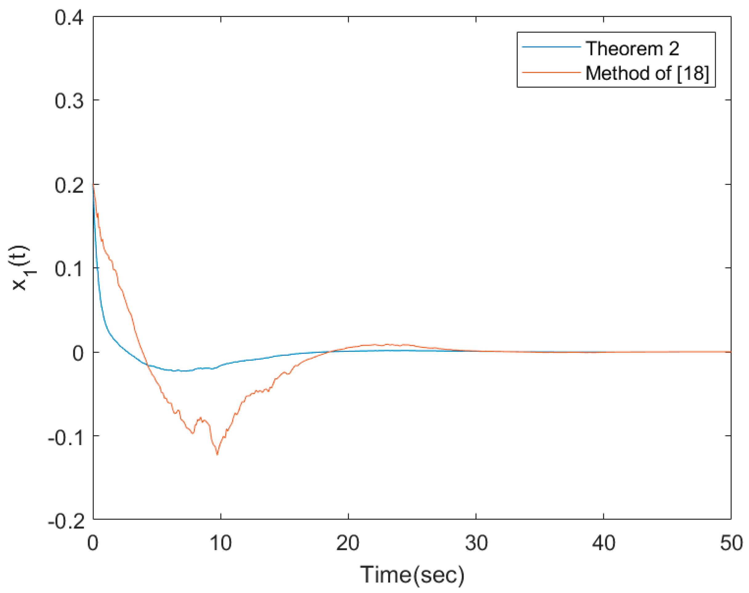
18] is applied to design the following PDC-based output controller for the system (22)–(23).
where
and
. Based on the controller in (24), the response of
of the system (22)–(23) is stated in
Figure 1 with the initial condition as
. The following feasible solutions are found by satisfying the condition in (16) in Theorem 2:
To demonstrate the satisfaction of (19), the obtained feasible solutions in (25) are applied to ensure the following inequality:
Based on the solutions in (25), the PDC-based output feedback controller is designed as follows:
Along with the designed controller in (26), the responses of
of the system (22)–(23) are also presented in
Figure 1 with the same condition. Referring to
Figure 1, although stability can be achieved, the poor response of the system (22)–(23) driven by the controller in (26) is provided according to the stochastic behavior. Moreover, the transient response of the system (22)–(23) driven by the designed controller in (26) is better than one driven by (24).
Regarding robustness, the responses of the system (22)–(23) driven by the fuzzy controller in (26) are stated with three initial conditions as
,
, and
in
Figure 2,
Figure 3,
Figure 4,
Figure 5 and
Figure 6. As shown in
Figure 2,
Figure 3,
Figure 4,
Figure 5 and
Figure 6, all states of (22)–(23) with different initials converge to zero, although the only measured output signals are used as feedback signals. The vibrations in those figures are caused by their stochastic behavior. Thus, the proposed design method is less conservative than the method of [
18]. Moreover, the system (22)–(23) driven by the controller in (26) provides better transient response than the one driven by the controller designed by the method of [
18].
In order to emphasize the advantage of the output feedback controller, the control method in [
27] is applied to design a state-feedback controller. In [
27], all states are assumed as measurable and applied to design the fuzzy controller. Based on the method of [
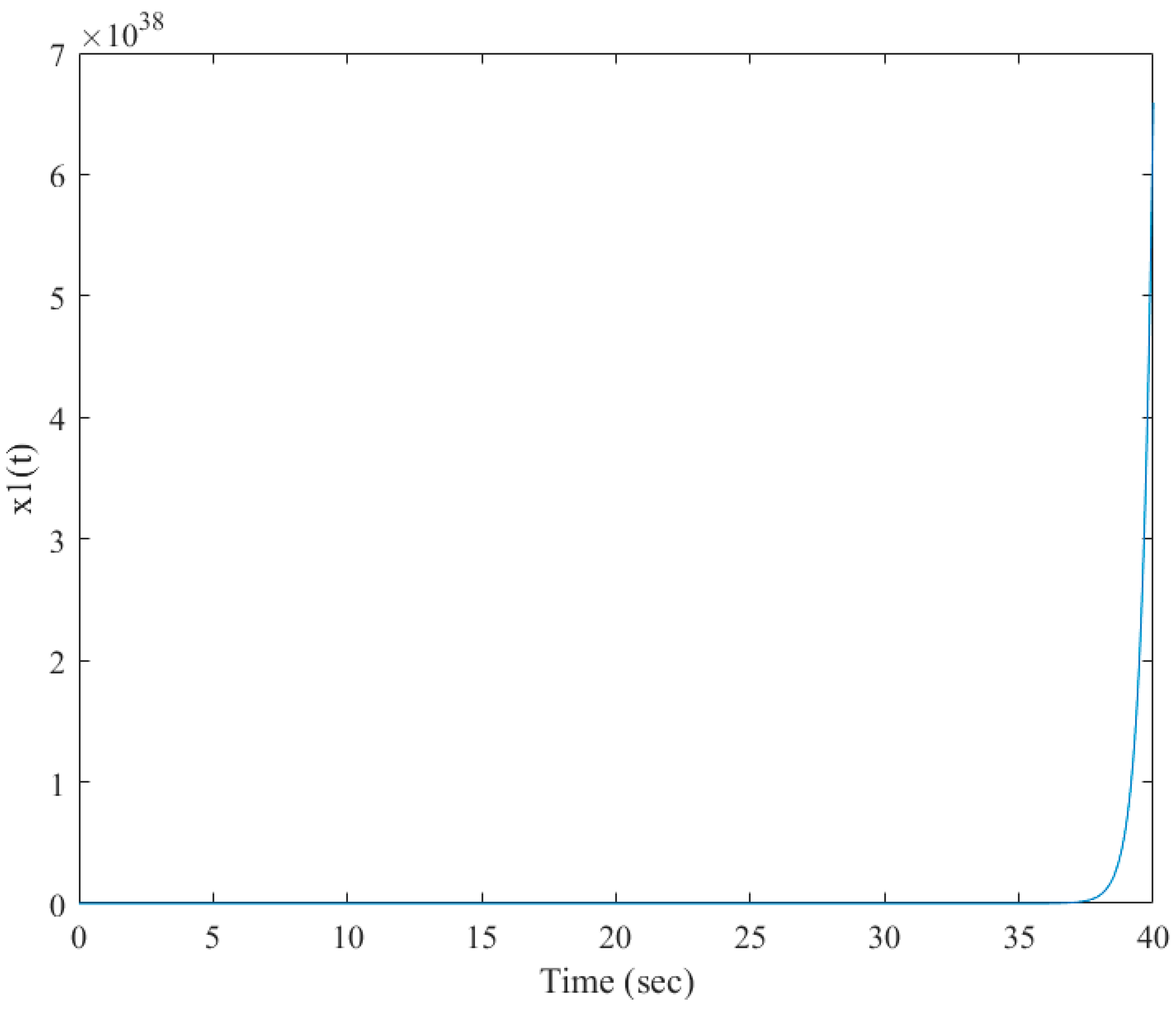
27], the fuzzy controller can be designed as follows:
where
and
.
With the fuzzy controller in (27) designed by [
27], the response of
shown in
Figure 7 cannot converge on zero. Therefore, the proposed design method is meaningful and practical for the control problem of nonlinear stochastic systems with unmeasurable states. Moreover, the asymptotical stability of nonlinear stochastic systems with unmeasurable states can be guaranteed by the proposed static output controller design method.


