Enhanced Variable Neighborhood Search-Based Recovery Supplier Selection for Post-Disruption Supply Networks

Abstract

With the increasing reliance on global sourcing and the growth in the likelihood of disruptive incidents, today’s supply networks are more prone to unexpected natural and man-made disruptive events. In order to alleviate the losses caused by these disruptive events, when a large-scale event disrupts multiple suppliers simultaneously, a single or several critical suppliers should be selected from the disrupted ones to assist them to recover their production as soon as possible. The selection of these recovery suppliers is of great importance in the recovery process of the entire supply network. Thus, this paper proposes a recovery supplier selection method from the view of the supply network structure. Firstly, a tripartite graph-based supply model is proposed to depict a two-stage supply network, which consists of multiple manufacturers and suppliers as well as the diverse product supply-demand interdependence connecting them. To measure the impacts caused by supplier disruptions and to evaluate the effectiveness of recovery supplier decisions, two supply network performance metrics reflecting product supply availability are also given. Then, the recovery supplier selection problem is described as a combinatorial optimization problem. To solve this problem, a heuristic algorithm, with enhanced variable neighborhood search (EVNS) is designed based on the general framework of a variable neighborhood search. Finally, experiments based on a real-world supply network are conducted. The experimental results indicate that the proposed method is applicable and effective.

1. Introduction

Recently, supply network managers have become increasingly concerned with disruptions to their systems, especially events that have the potential to disrupt multiple components of the supply network. Over the past 20 years, there have been many large-scale disruptive events, both man-made and natural [1,2]. For example, recently, the outbreak of the COVID-19 virus affected supply networks globally [3]. Early in March 2020, the number of COVID-19 cases had grown exponentially all over the world, resulting in border closures, quarantines, and full shut-downs of many crucial facilities, markets, and activities in the supply networks. As a result, product supply availability in global supply networks has been drastically reduced. A related survey indicates that the 1000 largest enterprises in the world have been severely impacted by COVID-19 [4].

In order to reduce losses caused by these large-scale supply network disruptions, management strategies have to be applied [5]. For example, in 2011, as a result of the Great East Japan earthquake, multiple automobile suppliers were severely damaged including the giant automotive semiconductor supplier, Renesas Electronics. Due to the earthquake, its main plant in the Naka region halted its production. The supply of automotive semiconductors was expected to cease for eight months. In order to recover the production of its main plant as soon as possible, Toyota and several other Japanese automobile and electronic equipment manufacturers sent more than 2500 engineers to support the recovery of its main plant. As a result, the recovery time of its main plant to start supplying automobile semiconductors was shortened from eight to five months [6]. Another example was the case of the Riken Corporation, which is the largest piston ring supplier in Japan. In July 2007, a Riken plant in the city of Kashiwazaki was damaged badly by a strong earthquake. Without delay, under the coordination of Toyota, several Japanese automobile manufacturers sent an aid team of nearly 700 people to assist in the production recovery. As a consequence, the production of piston rings was stopped for two weeks only [7].

These real-life cases illustrate a typical disruption recovery method for supply networks, namely recovery supplier selection. Recently, lean management strategies, like reducing inventory and backup suppliers, leave supply networks fragile in the case of a disaster or catastrophe [8]. When suppliers are damaged by natural or man-made disasters simultaneously, the downstream firms have to apply strategies to minimize the loss caused by the product supply shortage, such as seeking alternative sources and assisting the disrupted suppliers to recover their production. However, a qualified substitute supplier can be very difficult to find in a short time, especially for some critical products. A recent study of the exposure level of the Ford Motor Company found that the disruption of some critical suppliers leads to significant profit losses because they are difficult to quickly replace [9]. In addition, an alternative supplier can be much more expensive. In such a context, assisting disrupted suppliers to recover their production can be beneficial, alleviating the impact of disruptions effectively and efficiently. Due to the limitation of cost, it is impossible to assist all disrupted suppliers to recover their production. To find an optimal selection of recovery suppliers, studies have been proposed [10,11,12,13]. However, these previous works are mainly from the local or dyadic perspective, they pay little attention to the connectivity pattern of entities within a supply network, namely the supply network structure.

Recently, some researchers indicate that the management of supply network disruptions needs to take the structure of supply networks into consideration [14,15]. With the development of global trading and learnings in manufacturing, today’s supply networks can be huge and complex [16]. As some researchers defined, supply networks are interconnected structures that emerge from a largely downstream exchange of goods between firms (i.e., manufacturers, distributors, retailers, etc.) that are involved in creating a set of final products [17]. For example, the supply network of a large-scale enterprise may have multiple manufacturers and these manufacturers are connected with multiple suppliers by various product supply-demand relations. In the case studied by Sabouhi et al. [18], Atra Pharmaceutical Company (APC), which is an affiliation of Tamin Pharmaceutical Investment Company (TPICO), has multiple manufacturers across five Iranian provinces and these manufacturers purchase from multiple suppliers. In such a context, the disruption or recovery of a single or a few suppliers could influence the function of the entire system greatly. For example, the disruption of a supplier supplying various products to many manufacturers can damage the whole supply network greatly, since the disruption may result in the cessation of product supply from multiple manufacturers. In the same way, when selecting a few disrupted suppliers to recover their production, it seems more beneficial to select suppliers connected with multiple manufacturers. Thus, when decision-makers such as supply network managers or supply network service companies select the recovery suppliers for a post-disruption supply network, it is necessary to consider the macro network structure.

Based on these past works, this study investigates the recovery supplier selection problem from the perspective of the supply network structure. Firstly, to depict a two-stage supply network, which is composed of multiple manufacturers and suppliers as well as the diverse product supply-demand interdependences connecting them, a model using a tripartite graph is presented. Performance metrics describing product supply availability are also designed for assessing the damage caused by supplier disruptions and evaluating the effectiveness of recovery supplier decisions. Then, the problem of recovery supplier selection is formulated. Based on the variable neighborhood search (VNS) framework, an enhanced variable neighborhood search (EVNS) is proposed to solve the problem. Finally, to validate the effectiveness of the proposed method, experiments based on a real-world supply network are also conducted.

In the remainder of this paper, Section 2 provides a review of related works. The proposed supply network model and corresponding performance metrics are described in Section 3. Section 4 illustrates the EVNS-based recovery supplier selection method. Section 5 gives the case example to validate the proposed method. Section 6 concludes this paper.

2. Related Works

Supply network disruptions are usually defined as unexpected events that hamper the functioning of a supply network [19,20]. They can generally be divided into two types: random disruptions and target disruptions [21,22,23]. Random disruptions correspond to unintentional incidents, like natural disasters, accidents, public health events, etc. Target disruptions refer to intentional attacks, like a military or terrorist attack. In the past decades, supply network disruptions happen more and more frequently. At the same time, damages incurred by these disruptive events are also more severe than ever. According to related reports, almost 75% of enterprises suffer at least one supply network disruption per year [24].

To mitigate the damages caused by supply network disruptions, it is essential to apply management strategies, which mainly fall into two categories, namely proactive and reactive strategies [25]. Proactive strategies refer to those performed before the occurrence of disruptions. They are aimed at enhancing the resistant ability of a supply network in the presence of disruptions, such as adding redundancy [26], fortification of suppliers [27], and contracting with backup suppliers [28]. Reactive strategies are those conducted after the occurrence of disruptions. They are focused on recovering the function of a post-disruption supply network as soon as possible, such as contingent rerouting [29] and recovery supplier selection [13]. Most of the previous disruption management researches are from the perspective of a dyad or locally. Recently, with the increasing awareness of the complex supply network structure, some researchers point out that disruption analysis and management should take the supply network structure into consideration [15,30,31]. In the meanwhile, a complex network provides an efficient tool to characterize the structure of a supply network and conceptualize disruptive events. Thus, supply network disruption management researches based on complex networks have emerged continuously during the past years.

Due to the facilitation of complex network modeling methods, the complex supply network structure can be depicted as a collection of nodes and edges [32,33,34]. Nodes denote entities like manufacturers and suppliers. Edges represent the interdependent relations between entities such as product supply-demand relations, cooperative relations, and so on. Using complex network modeling and analysis methods, researchers try to analyze and mitigate supply network disruptions from the level of the network structure [15,35,36,37]. Generally, these complex network-based supply network disruption management researches can be classified into two categories. The first category focuses on finding an optimal structure of supply networks, which can withstand various types of disruptions. For example, Zhao et al. designed two heuristic strategies to build, design, or adjust the supply network structure and evaluated them against random and targeted disruptions [21,22,23]. Shi et al. proposed a supply network evolutionary model to generate a robust supply network structure, which can resist both random and target disruptions simultaneously [38]. Deng et al. presented a supply network structural optimization method to enhance the robustness of existing supply networks against target attacks [39]. The second category concentrates on using network centrality metrics to identify the vulnerabilities within a supply network. For example, Mizgier proposed a bottleneck identification method to identify entities whose disruptions will inflict the greatest damage to the entire network [40]. Ledwoch et al. presented a risk identification method using network centrality metrics [41]. Yan et al. designed comprehensive supplier evaluation metrics based on several network centrality metrics to detect the suppliers occupying the central positions in the network [42,43].

These previous studies have made significant contributions to mitigate disruptions from the perspective of the supply network structure. However, these studies still have several limitations. Firstly, the modeling methods adopted in these previous studies neglect the important role of products in the supply networks. Most of these works assume that supply networks are homogeneous. They treat all entities in a supply network as equal. Although some researchers consider the role difference between demanders and suppliers [21,22], they still ignore the difference of products supplied by different suppliers. In the meanwhile, some researchers point out that modeling methods without consideration of the products might be misleading in the analysis of disruptions [44]. As we know, supply networks form and function in order to transmit products or materials that make up an end product [36,45]. These products or materials can be distributed among the suppliers heterogeneously. That is to say, a product can be supplied by many suppliers, and a supplier could also supply many types of products. Compared with a supplier only supplying a few types of products, the disruption of a supplier supplying many types of products can impact the supply network more significantly. The supply network models without consideration of the products will not reflect such a consequence. Reviewing those high-impact supply network disruptive events, most of them are related to the stoppage of product supply. Secondly, these previous works mainly consider enhancing the supply networks’ resistance ability in the face of disruptions, lacking research exploring how to respond and recover from disruptions from the view of the supply network structure. Nevertheless, there are expectations for disruption recovery methods. Since disruptions refer to catastrophic events that are difficult to predict and control, it seems impossible to eliminate them no matter how many precautionary actions have been implemented [46]. In such cases, appropriate recovery strategies are more suitable for tackling these unpredictable disruption risks and making the supply network more resilient [47].

Based on these previous works, this paper contributes to developing a recovery supplier selection method from the network structure viewpoint. In this study, a network considering both the differing roles of manufacturers and suppliers and the diversity of product supply-demand relations between them is proposed. Facilitated by the proposed supply network model, performance metrics reflecting product supply availability are designed. Then, a reactive disruption management method, EVNS-based recovery supplier selection, is proposed, of which the effectiveness is validated using a real industry case.

3. Supply Network Model and Performance Metrics

3.1. Tripartite Graph-Based Supply Network Model

A “full-spectrum” supply network can be treated as a large-scale “ecosystem”, which is formed by many diverse entities, like suppliers, manufacturers, retailers, and customers [22]. In this study, we will investigate a typical two-stage supply network consisting of manufacturers, suppliers, and the product supply-demand relations between them. This is a commonly used structure in many previous works [48,49].

To distinguish the different roles of manufacturers and suppliers as well as the various product supply-demand relations between them, the two-stage supply network is described as a directed tripartite graph G = {V_M, V_P, V_S, E^PM, E^SP}, where the V_M, V_P, and V_S are three non-overlapping and independent node sets, E^PM and E^SP are two disjoint edge sets.

V_M = {m₁, m₂, …, m_NM} is the manufacturer node-set, denoting manufacturers in the network. V_P = P(m₁)∪P(m₂)∪P(m₃), …, ∪P(m_NM) is the product node-set, representing the necessary products demanded by the manufacturers. P(m_i) = {p_i^k| k=1, 2, …, |P(m_i)|} denotes the necessary products demanded by m_i, where p_i^k refers to the k-th necessary product for m_i. V_S = {s₁, s₂, …, s_NS} is the supplier node-set, denoting suppliers in the network.

E^PM = {(p_i^k, m_i)| p_i^k∈V_P, m_i∈V_M} is the product demand edge set, describing the demand relations between the necessary products and manufacturers. In E^PM, a given directed edge (p_i^k, m_i) denotes the demand relation between manufacturer m_i and product p_i^k. E^SP = {(s_j, p_i^k)| s_j∈V_S, p_i^k∈V_P} is the product supply edge set, representing the supply relations between products and suppliers. In E^SP, a given directed edge (s_j, p_i^k) refers to the supply relation between supplier s_j and product p_i^k.

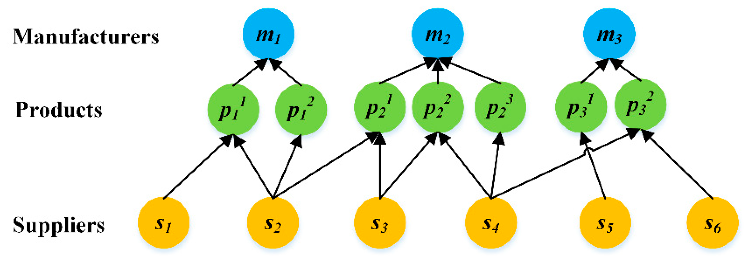
As shown in Figure 1, a simple example is given to illustrate the proposed supply network model. In the figure, three types of entities, manufacturers, products, and suppliers are marked by blue, green, and yellow respectively. Each manufacturer needs several different types of products to perform its own production duty. Suppliers supply these necessary products to satisfy the manufacturers’ demands. For instance, manufacturer m₁ needs two types of products, which are denoted by p₁¹ and p₁². In the meanwhile, supplier s₁ supplies products p₁¹ to m₁, supplier s₂ supplies both p₁¹ and p₁² to m₁. Hence, (p₁¹, m₁) and (p₁², m₁) are two product demand edges. (s₁, p₁¹), (s₂, p₁¹) and (s₂, p₁²) are three product supply edges.

3.2. Performance Metrics

Recovery supplier selection refers to selecting a limited number of suppliers from the disrupted ones, whose recovery will increase the performance of a post-disruption supply network most effectively [11]. Proper performance metrics are needed to measure the damage induced by supplier disruptions and to evaluate the effectiveness of recovery supplier selection decisions.

Previous researches hold the opinion that the transmission of products is the basic duty of a supply network. The failure of delivering products to demanders who need them can be treated as performance decrements of supply networks [50]. Additionally, real cases indicate that product supply stoppage is one of the main reasons that cause huge losses for supply networks. For example, several hard disc suppliers were damaged severely in the 2011 Thailand flooding, which lead to the supply stoppage of hard discs globally. As a consequence, the production of many computer manufacturers had to halt their production [51]. In the same year, automobile manufacturer Nissan suffered a lot in the 2011 Great East Japan earthquake. A critical engine supplier of Nissan was destroyed in the earthquake. This forced a Nissan plant in the UK to shut down for three days due to the supply shortage of engines [52]. Based on these considerations, two performance metrics describing product supply availability, namely the product supply availability rate and the manufacturer filling rate, are given in this section.

Firstly, we introduce the definition of the product supply availability rate. As mentioned above, the duty of a supply network is to deliver necessary products to their demanders. In the supply network model considered in this research, each product node represents a type of necessary product demanded by a manufacturer. If a product node loses all of its supply edges, it means the failure to deliver a type of product to the corresponding demanders. Thus, to reflect the ability of a supply network to deliver necessary products to their demanders, the product supply availability rate is defined as the percentage of product nodes in the network having access to supplier nodes. The calculation of the product supply availability rate is given using Equation (1).

$$r_A=\frac{1}{\left|V_P\right|}{\displaystyle \sum }_{p_i^k\in V_P}\epsilon \left[\left|{\phi }_S\left(p_i^k\right)\right|\right]$$

(1)

$$\epsilon \left[\left|{\phi }_S\left(p_i^k\right)\right|\right]=\{\begin{array}{c}1,if \left|{\phi }_S\left(p_i^k\right)\right|>0\\ 0,if \left|{\phi }_S\left(p_i^k\right)\right|\le 0\end{array}$$

(2)

where |V_P| denotes the total number of product nodes in the network. |φ_S(p_i^k)| denotes the number of supplier nodes attached to p_i^k. When |φ_S(p_i^k)| > 0, it means that product p_i^k can be delivered from the suppliers to the corresponding demander m_i. When |φ_S(p_i^k)| = 0, it represents that product p_i^k can not be delivered to its demander m_i.

Then, the definition of the manufacturer filling rate is presented. In a supply network, manufacturers depend on their suppliers to obtain the necessary products for producing their own products. For a given manufacturer, it will not be able to produce its own products unless it can obtain all the necessary products. Hence, the manufacturer filling rate is defined as the percentage of manufacturers who can obtain all necessary products to produce their own products. The calculation of the manufacturer filling rate is presented using Equation (3).

$$r_F=\frac{1}{\left|V_M\right|}{\displaystyle \sum }_{i=1}^{\left|V_M\right|}\delta \left[r\left(m_i\right)-1\right]$$

(3)

$$r\left(m_i\right)=\frac{1}{\left|P\left(m_i\right)\right|}{\displaystyle \sum }_{k=1}^{\left|P\left(m_i\right)\right|}\epsilon \left(\left|{\phi }_S\left(p_i^k\right)\right|\right)$$

(4)

$$\delta \left[r\left(m_i\right)-1\right]=\{\begin{array}{c}1,if r\left(m_i\right)-1=0\\ 0,if r\left(m_i\right)-1\ne 0\end{array}$$

(5)

where |V_M| is the total number of manufacturer nodes in the network. r(m_i) describes the level of m_i to obtain all the necessary products. When r(m_i) = 1, it means that manufacturer m_i can obtain all necessary products to produce its own products. When r(m_i) < 1, it refers to manufacturer m_i being unable to obtain all the necessary products to perform their production duty.

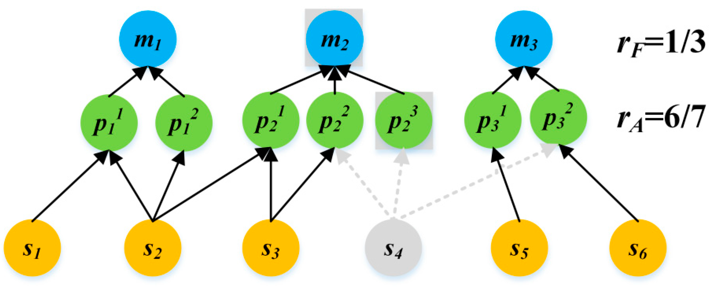
Figure 2 gives an example to explain the calculation of two proposed performance metrics. As presented in the figure, the disruption of supplier s₄ leads to manufacturer m₂ failing to obtain product p₂³. According to the definition of product supply availability rate and manufacturer filling rate, r_A and r_F of the supply network shown in Figure 2 are 6/7 and 1/3 respectively.

4. Enhanced Variable Neighborhood Search-Based Recovery Supplier Selection

After introducing the supply network model and performance metrics, this section illustrates the EVNS-based recovery supplier selection method. First, the problem of recovery supplier selection is described. Then, the EVNS algorithm is designed to solve the problem, of which the details are presented.

4.1. The Recovery Supplier Selection Problem

4.1.1. Problem Statement and Assumptions

In this subsection, the problem statement and assumptions of recovery supplier selection are provided.

Firstly, the problem is stated. This study considers the recovery supplier selection problem under high-impact disruptive events from a perspective of network structure. When a large-scale disruptive event descends upon a supply network, such as the outbreak of virus COVID-19, multiple suppliers can be damaged simultaneously. To alleviate the losses caused by the product supply shortage, decision-makers could assist the disrupted suppliers to recover their production for reattaining the product supply as soon as possible. However, the cost for assisting suppliers’ recovery is limited, therefore, it is impossible to assist all disrupted suppliers. A single or several critical suppliers need to be selected as recovery suppliers in such a way that the recovery process of the entire supply network is optimized [13]. Based on the supply network model and performance metrics proposed in this study, the recovery supplier selection problem can be described as selecting a limited number of suppliers from the disrupted ones, of which the recovery can increase both performance metrics r_A and r_F of the post-disruption supply network most greatly.

Then, assumptions are presented. To simulate supplier disruptions, the node failure model is adopted [17,31,32,38], which describes the disruption of a supplier node as the total failure of it. Besides, this study is focused on the disruption management of supply networks from a macro system level, the autonomous individual behaviors from a micro level are not considered. Such simplification is common in similar systems such as epidemiology or food webs. In some previous works from the field of supply networks, researchers also neglect the micro individual behaviors to focus on a macro network-level analysis of the supply network [22,23,39]. Thus, the following assumptions are made.

Assumption 1:

Once a supplier is disrupted, it will lose all the production ability, which causes all its product supply edges to be removed in the network.

Assumption 2:

Spontaneous recovery behaviors of disrupted suppliers are neglected. Once a supplier is disrupted, the production ability of it will not be recovered unless it is selected to be a recovery supplier.

Assumption 3:

Autonomous individual behaviors of both manufacturers and suppliers, such as coordination, are neglected.

Assumption 4:

When a disrupted supplier is selected as a recovery supplier, the production ability of it will be fully recovered. The product supply edge of it will be rebuilt according to the structure of the original network without disruptions.

Assumption 5:

The cost for recovering each disrupted supplier is assumed to be equal. Thus, the number of selected recovery suppliers is used to denote the limited recovery cost.

An example to illustrate the disruption and recovery of suppliers is given in Figure 3. As shown in Figure 3a, supplier s₁, s_2, and s₆ are disrupted in the network. The supply edges of these disrupted suppliers are removed, which are marked in grey. In Figure 3b, s₂ is selected from the three disrupted suppliers to be a recovery supplier. It can be observed that the recovery of s₂ is modeled by rebuilding its product supply edges. Comparing Figure 3a,b, it can also be observed that different recovery supplier decisions can result in very different results. For example, after the recovery of s₂, r_A and r_F of the recovered network are 6/7 and 2/3 respectively. If we select s₁ as the recovery supplier, r_A and r_F of the recovered network will be 5/7 and 1/3. This also indicates the necessity of investigating the recovery supplier selection problem from the network structure view.

4.1.2. Mathematical Model

For a residual supply network after the disruption of a supplier set D, denoted by G’, the recovery supplier selection for network G’ means searching for a limited supplier subset I from D, the recovery of which will increase both performance metrics r_A and r_F most evidently. This is a typical combinatorial optimization problem, which can be formulated as below:

$${\mathrm{Max}}_{I}H\left(I\right)$$

(6)

$$H\left(I\right)=\theta \times r_A\left({G_I}^{\prime }\right)+\left(1-\theta \right)\times r_F\left({G_I}^{\prime }\right)$$

(7)

$$\mathrm{Subject} \mathrm{to} I\subseteq D$$

(8)

$$\left|I\right|=K_R$$

(9)

where I denotes a recovery supplier subset selected from the disrupted supplier set D. |I| is the number of suppliers in set I. K_R is a pre-set integer, representing the limited recovery cost. Constrain (8) means that recovery suppliers have to be selected from the disrupted ones. Constrain (9) represents that the number of selected recovery suppliers is constrained by limited recovery costs, namely the predefined integer K_R. G_I’ denotes the network G’ after the recovery of supplier set I. r_A(G_I’) and r_F(G_I’) denote the product supply availability rate and manufacturer filling rate of the recovered supply network G_I’ respectively. The objective function (7) refers to a comprehensive performance evaluation of network G_I’. θ is a tunable parameter. When 0 ≤ θ < 0.5, the supply network performance generally relies on the manufacturer filling rate. When 0.5 < θ ≤ 1, the supply network performance mainly depends on the product availability rate. Since both product supply availability rate and manufacturer filling rate are considered to be equally important in this study, θ is set to be 0.5. The objective function (7) will be used for fitness evaluation in the following EVNS algorithm.

4.2. Enhanced Variable Neighborhood Search

The recovery supplier selection is formulated as a combinatorial optimization problem in Section 4.1. According to previous researches, there are two types of methods to solve such a problem, exact and heuristic algorithms. In theory, exact algorithms can provide an optimal solution together with the proof of its optimality. However, many practical instances of combinatorial problems, arising in operations research and other fields, are too great for an exact solution to be found in an acceptable time. Meanwhile, heuristic algorithms provide another option, since they are capable of finding approximate solutions with high quality within a reasonable time.

VNS is a type of heuristic framework, which is known for its simplicity and flexibility [53]. The main idea behind VNS is that a local optimum in one neighborhood may not be a local optimum in other neighborhoods. This allows the algorithm to perform a powerful intensification of local searches. Therefore, a heuristic algorithm, EVNS is designed based on the general VNS framework to solve the recovery supplier selection problem. The following sections will present the details of it.

4.2.1. Solution Representation and Fitness Evaluation

In the proposed EVNS, each feasible solution of the recovery supplier selection problem is coded using string. Any feasible solution, namely a subset of selected recovery suppliers, can be represented by a string I={I(1), I(2), …, I(K_R)}, where I(i) denotes a supplier selected from the disrupted supplier set D. K_R is the pre-set integer, denoting the limited number of selected recovery suppliers. An example is given in Figure 4 to illustrate the string-based solution coding method. As shown in the figure, the suppliers marked by light blue boxes represent the selected recovery suppliers. Using the string-based coding method, the selected recovery suppliers are presented by {1, 4, 6}.

To solve the recovery supplier selection problem, operations will be performed to find the recovery supplier subset from the disrupted supplier set whose recovery will improve both performance metrics of the post-disruption supply network most evidently. Hence, each solution needs to be assessed by a fitness value. In this study, solutions with higher fitness values are considered to be better than those with lower fitness values. According to the optimized object, the fitness value of a given solution I can be calculated using the objective Equation (7).

4.2.2. The General Framework of an EVNS

The proposed EVNS is composed of two main procedures: initialization and a two-stage solution improvement. After the initialization of the solution (Section 4.2.3), EVNS will iterate a two-stage solution improvement procedure until the terminal condition is met, which contains a recovery degree-based local neighborhood search, an enhanced local neighborhood search, and a secondary optimization-based neighborhood changing scheme. The recovery degree-based local neighborhood search is composed of a recovery degree-based local neighborhood structure determination (Section 4.2.4) and an exchanging-based search (Section 4.2.6). The enhancing local neighborhood search is made up by enhancing local neighborhood structure construction (Section 4.2.5) and an exchanging-based search (Section 4.2.6). The secondary optimization-based neighborhood changing scheme decides the alternation between the two local neighborhood searches. In each solution improvement procedure, the recovery degree-based local search will be performed first. If an improved solution is found in the recovery degree-based local search, the enhancing local search will be applied to optimize the improved solution further. Otherwise, the enhancing local search will not be performed. The flowchart and main procedures of the EVNS are given in Figure 5 and Algorithm 1. The key procedures will be presented in the following sections.

Algorithm 1. Enhanced variable neighborhood search (EVNS)

Input:G’, G, D, KR, NPOP, Ncandidate Output: I  I ← Initialization(G’, G, D, KR, NPOP)  while (end condition is not met)   %Recovery degree-based local search   Scandidate ← Recovery degree-based local neighborhood structure(G’, G, D, I, Ncandidate)   I* ← Exchanging-based search(G’, G, I, Ncandidate, Scandidate)   if fitness(I*)>fitness(I)    I←I*    % Enhancing local search    Scandidate ← Enhancing local neighborhood structure(G’, G, D, I, Ncandidate)    I* ← Exchange-based search(G’, G, I, Ncandidate, Scandidate)    if fitness(I*)>fitness(I)     I←I*    end   end  end Return:I

4.2.3. Initialization

Like most heuristic algorithms, the quality of an initial solution can affect both the solution quality and the converging speed of the EVNS. Thus, a high-quality initial solution is of great importance. To guarantee the high quality of an initial solution, a random search will be performed. As shown in Algorithm 2, the initialization contains two steps. Firstly, a random solution generation procedure is applied to obtain multiple feasible solutions within the entire solution space. Then, the best one is selected from the randomly generated solution set as the initial solution.

Algorithm 2. Initialization

Input:G’, G, D, KR, NPOP Output: I  POP = Ø   while t < NPOP    It ← Select KR supplier nodes from D randomly    if It ∩ POP = Ø     POP = POP∪{It}    end   end   I ← argmaxIt fitness(It) Return:I

4.2.4. Recovery Degree-Based Local Neighborhood Structure

Local neighborhood search refers to a procedure to optimize the quality of a solution by modifying part of it. The neighborhood structure can affect the performance of it greatly. The recovery supplier selection problem concerned in this research means selecting a limited supplier node subset I from the disrupted supplier node-set D, of which the recovery will increase both performance metrics r_A and r_F the most greatly. This can be treated as a variant of the critical node selection problem. A traditional neighborhood for the critical node selection problem is defined by the conventional exchange operator which swaps a node s_x∈I with a node s_y∈D\I [54]. For a given solution I, this neighborhood yields K_R×(|D|-K_R) neighbor solutions. Examining the entire neighborhood can be quite time-consuming.

To narrow the search scope and to concentrate on the optimization objective, the recovery degree-based local neighborhood structure is constructed. The directed reason for performance decreasing of a supply network is product supply stoppage. Due to the disruption of partial suppliers, some product nodes lose all supply edges, leading to the dysfunction of corresponding manufacturer nodes further. In a similar way, the performance of a post-disruption supply network can also be improved by rebuilding product supply edges for those product nodes without supply edges. Thus, when considering exchanging supplier node s_x belonging to I with supplier node s_y belonging to D\I to improve I, it seems more proper to select s_y whose recovery can rebuild more supply edges for those product nodes without supply edges in the post-disruption supply network G’. Based on such a consideration, a recovery degree-based local neighborhood structure is constructed. As presented in Algorithm 3, there are two main steps:

• Calculate the recovery degree for each supplier node in set D/I. Recovery degree is defined as the number of product nodes without supply edges in G’ connected with a supplier node in the original network G. The expression of recovery degree is presented using Equation (10). A simple example is presented in Figure 6 to illustrate the calculation of the recovery degree. In the supply network presented in the figure, there are three disrupted supplier nodes s₁, s_2, and s₄. According to the definition of a recovery degree, the recovery degrees of these nodes are 1, 2, and 1 respectively. Among the three disrupted supplier nodes, s₂ has the highest value of recovery degree. And the recovery of s₂ can increase r_A and r_F of the entire network most evidently.

  $$V_R\left(s_j\right)=\left|P^{\prime }{\displaystyle \cap }{\phi }_P\left(s_j\right)\right|$$

  (10)

  where P’ refers to the product nodes without supply edges in network G’. φ_P(s_j) denotes the product nodes connected with s_j in original network G. |P’∩φ_P(s_j)| represents the number of product nodes in set P’∩φ_P(s_j).
• Set the candidate supplier set S_candidate as an empty set. Iterate the roulette wheel-based candidate supplier selection N_candidate times to add the selected suppliers into S_candidate. The possibility of a given supplier s_j being selected in a round of roulette wheel-based candidate supplier selection is presented using Equation (11).

  $$probility\left(s_j\right)=\frac{V_R\left(s_j\right)}{{\displaystyle {\displaystyle \sum }_{s_v\in D/I/S_{candidate}}}{V}_R\left(s_v\right)}$$

  (11)

Algorithm 3. Recovery Degree-based Local Neighborhood Structure

Input:G’, G, D, I, Ncandidate Output:Scandidate  for each sj∈D/I   calculate VR(sj) in G’ using Equation (10)  end  Scandidate = Ø  for t =1: Ncandidate   sadd← using roulette wheel selection to select a supplier from D/I/Scandidate   Scandidate = Scandidate∪{sadd}  end Return:Scandidate

4.2.5. Enhancing Local Neighborhood Structure

Searching in a single local neighborhood structure may fall into local optimums. Thus, this research also designs enhancing local neighborhood structure. Unlike a recovery degree-based local neighborhood structure, the construction of an enhancing local neighborhood structure considers searching the optimal recovery supplier nodes in the network after recovering I. As presented in Algorithm 4, the construction of an enhancing local neighborhood structure is composed of the following steps:

• The candidate supplier set S_candidate is set as an empty set.
• Calculate the recovery degree for each supplier node in set D/I/S_candidate in the network. G’_{I∪Scandidate}, and determine the node with the highest value of recovery degree as s_add.
• Add s_add into set S_candidate. Iterate step. 2 N_candidate times, until the set S_candidate contains N_candidate nodes.

Algorithm 4. Enhancing Local Neighborhood Structure

Input:G’, G, D, I, Ncandidate Output:Scandidate  Scandidate= Ø  for t=1: Ncandidate   G’I∪Scandidate ← Recovering I∪Scandidate in G’   for each sj∈D/I/Scandidate    calculate VR(sj) in G’I∪Scandidate using Equation (10)   end   sadd ← argmaxsj∈D/I/Scandidate VR(sj)   Scandidate = Scandidate ∪ {sadd}  end Return:Scandidate

4.2.6. Exchanging-Based Search

Section 4.2.4 and Section 4.2.5 present the construction of two local neighborhood structures by finding a set of candidate suppliers S_candidate in D/I. This section will present the searching strategy to generate candidate solutions by replacing part supplier nodes in I with some in S_candidate. To improve the searching efficiency, an exchanging-based search strategy is applied to generate the candidate solutions [54,55]. The main procedures of an exchanging-based search are presented in Algorithm 5. This strategy can be divided into two distinct phases. Firstly, the “nodes adding phase” adds the candidate recovery supplier node-set S_candidate into the solution I to generate a new solution I*. Then, the “nodes removing phase” is performed to remove a set of N_candidate supplier nodes from I*, which decreases the fitness value minimally. Figure 7 presents an example to illustrate the “nodes adding phase” and “nodes removing phase”.

Algorithm 5. Exchanging-based Search

Input:G’, G, I, Ncandidate, Scandidate Output:I*  % Nodes adding phase  I*=I ∪ Scandidate  % Node removing phase  for t = 1: Ncandidate   F= Ø   for each sj∈I*    F(sj) ← calculate fitness(I*/{sj})   end   sremove←argmaxsj∈I* F(sj)   I*←I*/{sremove}  end Return:I*

5. Case Example

This section presents a case example to evaluate the proposed EVNS-based recovery supplier selection method. Firstly, an empirical supply network is constructed. Then, experiments based on the empirical network are conducted to verify the effectiveness of the proposed method.

5.1. Empirical Supply Network

For the construction of an empirical supply network, product supply-demand data for the automotive industry was collected from Gasgoo automobile supplier database. Based on the database, users can query the suppliers by the supplied products or client names. Thus, data describing supply-demand relations between 47 manufacturers and 5579 suppliers involving 27 types of automobile products were obtained from the database.

Base on the collected data, an empirical supply network is built. Basic characters of the empirical supply network are presented in

Table 1. Basic characters of the empirical supply network.

Type	Subtype	Number
Node	Manufacturer Nodes	47
	Product Nodes	1269
	Supplier Nodes	5579
Edge	Product demand edge	1269
	Product supply edge	27,436

. It can be observed that the number of manufacturers is much higher than suppliers. The main reason is that a whole car is an extremely complex product, involving more than 5000 kinds of components. In addition, outsourcing is common in the automobile industry. A manufacturer relies on many suppliers for the assembly of whole cars. It is also found that there is an imbalance between the number of product demand edges and the number of product supply edges. The main reason is that manufacturers tend to adopt a multi-sourcing strategy to enhance their ability to resist supplier disruptions. Thus, a product node can be connected by multiple supplier nodes.

Previous works indicate that the degree distribution of a supply network can affect its robustness against disruption greatly [21,22]. Thus, the degree distribution of the empirical supply network is analyzed specifically. Figure 8a,b presents the degree distribution of product nodes and supplier nodes respectively. It can be observed that both of them can be fitted using a truncated power-law distribution [56]. Such highly skewed degree distribution indicates that supply networks in the real world are uneven. A very small number of entities occupy the central position in the network. Such results imply that supply networks in the real world can be vulnerable to the disruption of those intensively connected suppliers.

5.2. Evaluation of EVNS-Based Recovery Supplier Selection Method

The EVNS-based recovery supplier selection method will be evaluated in this section. Firstly, experiments are conducted for parameter tuning. Then, comparative experiments are made to compare the proposed method with others. To validate the effectiveness of the EVNS-based recovery supplier selection method further, the proposed two-stage solution improvement procedure is also evaluated. To achieve statistically significant results, each experiment was repeated 10 times. The final experimental results are calculated based on the independent 10 experiments. All experiments were performed using MATLAB R2014a (MathWorks, Natick, Massachusetts, USA) and run on a PC equipped with an Intel Core i7 and 16 GB of memory, running Windows 7.

5.2.1. Parameter Tuning

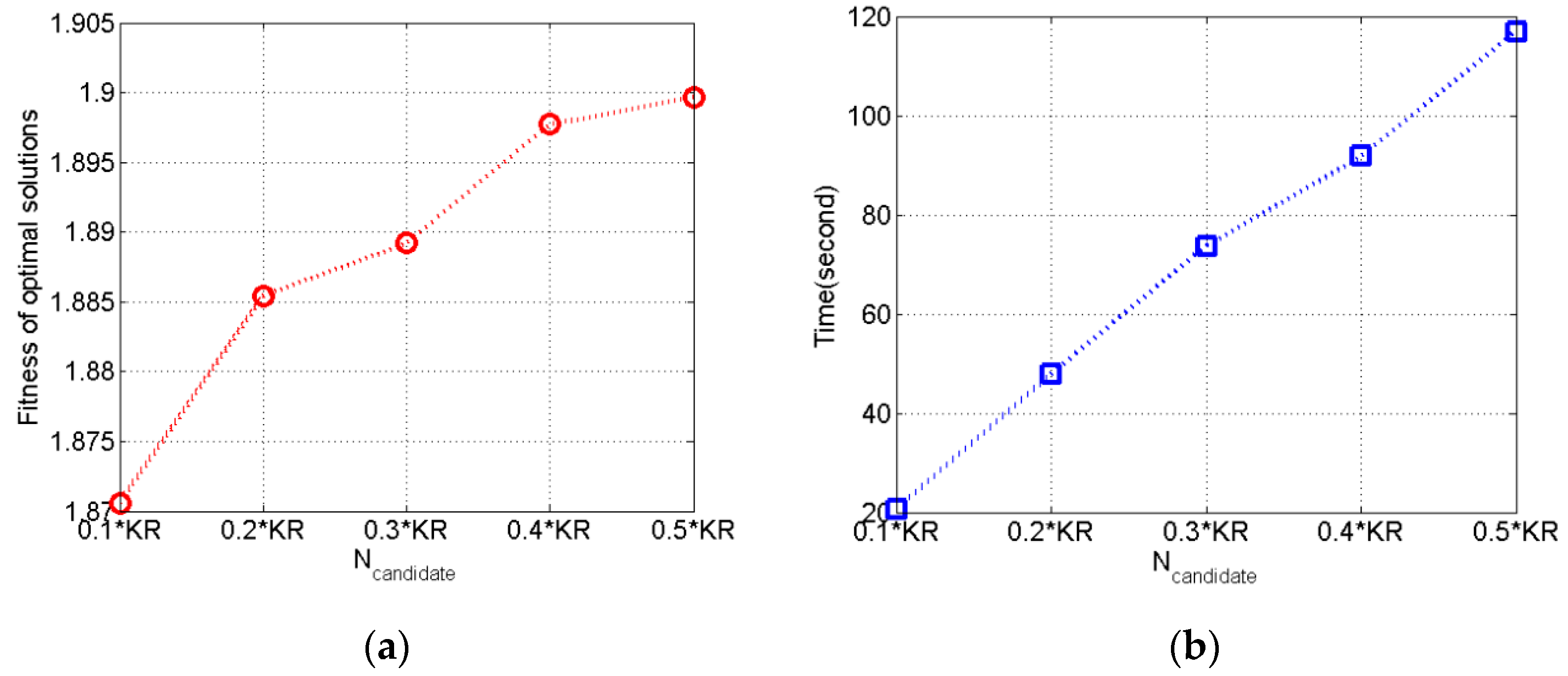
Like most heuristic algorithms, the performance of EVNS also relies on its parameters. As shown in Algorithm 1, EVNS only has two parameters N_POP and N_candidate. N_POP is set to be 100. To tune parameter N_candidate, we followed the common practice in the heuristic literature by testing a limited number of parameter configurations on a specific instance as follows. Firstly, the disruption scenario is set to be a random disruption of 3000 suppliers and the number of recovery supplier K_R is settled to be 10, namely this problem is used as a specific instance to determine the value of N_candidate. Then, the termination condition is set to be 30 generations. Experiments under the different values of N_candidate are conducted to analyze the impact of N_candidates upon the quality of optimal solutions and running time.

Figure 9 presents the experimental results. As shown in Figure 9a,b both the fitness value of optimal solutions and running time increase with the increase of N_candidates. It also has been noticed that the increment of fitness between 0.1 × K_R, 0.2 × K_R is most obvious. For ensuring both solution quality and time efficiency, N_candidate is determined to be 0.2 × K_R.

5.2.2. Comparative Experiments

To assess the EVNS-based recovery supplier selection method proposed in this research, comparative experiments are conducted. For the purpose of comparison, two types of recovery supplier selection methods are considered. The first type is network centrality-based target recovery methods, including degree centrality-based target recovery method (DC-TR) [57] and betweenness centrality-based target recovery method (BC-TR) [58]. The above methods use degree and betweenness centrality to rank the disrupted suppliers in descending orders and select the top-K_R suppliers as the recovery suppliers respectively. The second type includes heuristic algorithm-based recovery supplier selection methods, including Genetic Algorithm (GA) [59] and Greedy1 [60]. They are two general critical node detection algorithms. In this study, these two algorithms are used to solve the recovery supplier selection problem concerned in this research. The parameters of GA are set according to reference [59]. To be fair, GA and EVNS were running on our platform within the same maximal running time of 600 s.

To analyze whether the proposed method can adapt to different disruption scenarios, both random and target disruptions are taken into consideration. According to the previous works [21,22], random disruptions are modeled as the random failures of supplier nodes. Target disruptions are simulated using degree-based target failures of supplier nodes.

Since the number of recovery suppliers could impact the method performance, experiments under various values of recovery ratio (f_r) are also made. f_r is defined as the percentage of selected recovery suppliers to the number of the initial disrupted suppliers. The calculation of the recovery ratio is presented using Equation (12).

$$f_r=\frac{K_R}{\left|D\right|}$$

(12)

where |D| represents the number of initial disrupted suppliers, K_R represents the number of recovery suppliers.

Experimental Result under Random Disruption Scenario

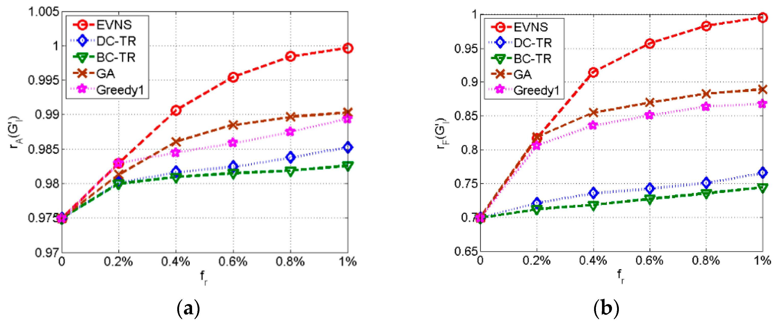
Figure 10 presents the experimental results under the random disruption of 3000 suppliers. Figure 10a,b show the comparisons of r_A and r_F recovery curves using different supplier recovery methods. As shown in Figure 10a, along with the increasing of f_r, all the recovery supplier selection methods can improve r_A more evidently. It can also be observed that the recovery effect of the EVNS-based method is much better than others. The experimental results presented in Figure 10b are similar to Figure 10a. It is also noticed that the recovering speeds of both r_A and r_F tend to slow down with the increasing of f_r.

For a quantitative comparison of different recovery supplier selection methods, the area under the r_A recovery curve (AUC_rA) and r_F recovery curve (AUC_rF) for each recovery supplier selection method is calculated.

Table 2. AUC_rA and AUC_rF comparison of different methods under the random disruption of 3000 suppliers.

	AUCrA			AUCrF
	Aver	Max	Min	Aver	Max	Min
EVNS	9.910 × 10−3	9.972 × 10−3	9.842 × 10−3	9.040 × 10−3	9.617 × 10−3	8.702 × 10−3
DC-TR	9.816 × 10−3	9.910 × 10−3	9.759 × 10−3	7.368 × 10−3	8.511 × 10−3	6.660 × 10−3
BC-TR	9.806 × 10−3	9.906 × 10−3	9.727 × 10−3	7.236 × 10−3	8.404 × 10−3	6.426 × 10−3
GA	9.856 × 10−3	9.941 × 10−3	9.786 × 10−3	8.445 × 10−3	9.362 × 10−3	8.021 × 10−3
Greedy1	9.846 × 10−3	9.911 × 10−3	9.779 × 10−3	8.283 × 10−3	9.064 × 10−3	7.851 × 10−3

reports the average values, the maximal values, and the minimum values of AUC_rA and AUC_rF of 10 repeated experiments. As shown in the table, the EVNS-based method achieves the biggest value for all indicators. Such results also validate the effectiveness of the EVNS-based recovery supplier selection method.

Experimental Results under the Target Disruption Scenario

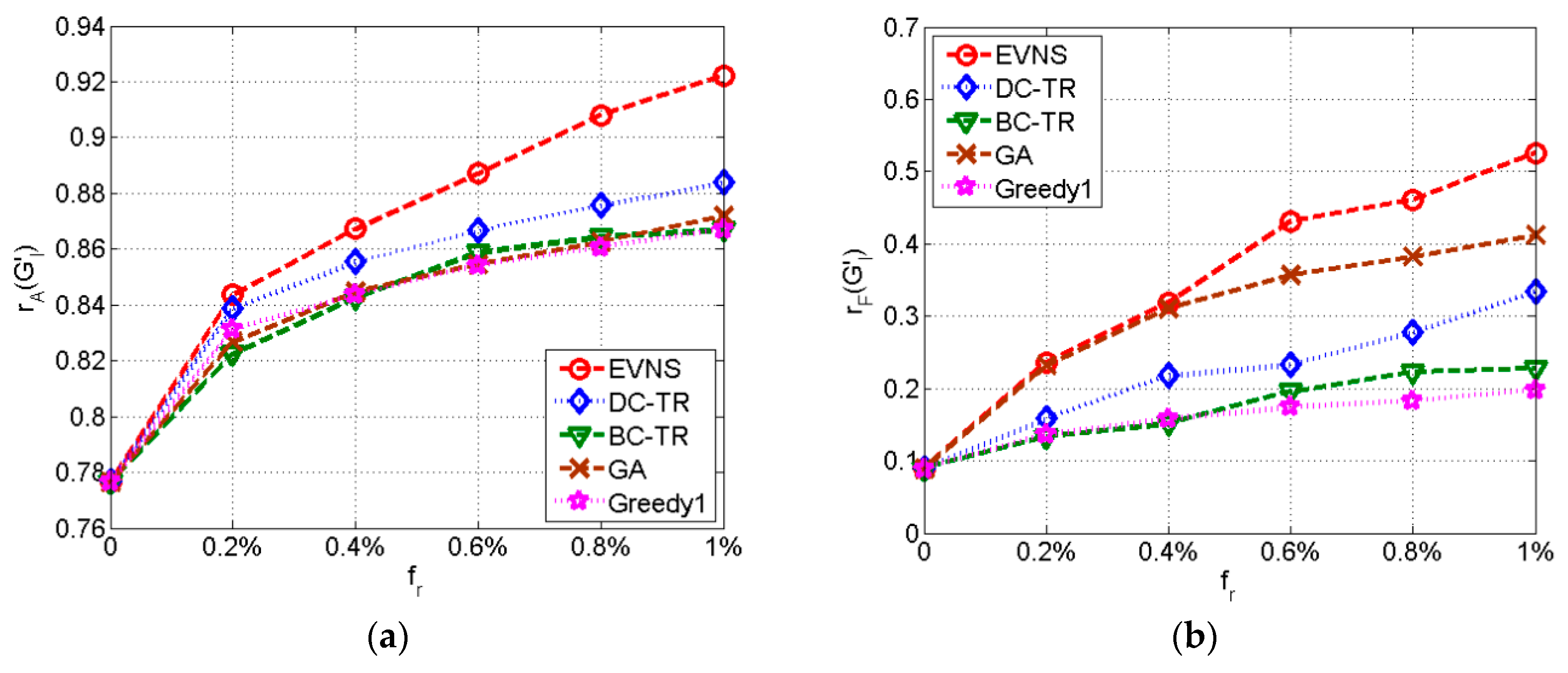
In anticipating random supplier disruptions, target supplier disruptions are also considered in the comparative experiment. Figure 11 presents the experimental results under the target disruption of 3000 suppliers. Figure 11a,b shows the r_A and r_F recovery curve comparisons using different supplier recovery methods under the target disruption of 3000 suppliers. The results presented in Figure 11 are similar to Figure 10. With the increasing of f_r, all the recovery supplier selection methods can improve both r_A and r_F more evidently. The EVNS-based method outperforms others. Comparing Figure 10 with Figure 11, it can be observed that target disruptions can induce much higher damage than random disruptions. This is caused by the skewed degree distributions of the empirical network. In the network, a very small number of suppliers provide many products to many manufacturers, and the disruption of these important suppliers may cause a large-scale product supply stoppage.

Table 3. AUC_rA and AUC_rF comparison of different methods under the target disruption of 3000 suppliers.

	AUCrA			AUCrF
	Aver	Max	Min	Aver	Max	Min
EVNS	8.711 × 10−3	8.772 × 10−3	8.690 × 10−3	3.513 × 10−3	4.043 × 10−3	3.128 × 10−3
DC-TR	8.532 × 10−3	8.569 × 10−3	8.508 × 10−3	2.189 × 10−3	2.383 × 10−3	1.872 × 10−3
BC-TR	8.419 × 10−3	8.456 × 10−3	8.380 × 10−3	1.726 × 10−3	1.936 × 10−3	1.362 × 10−3
GA	8.426 × 10−3	8.519 × 10−3	8.326 × 10−3	3.068 × 10−3	3.319 × 10−3	2.638 × 10−3
Greedy1	8.423 × 10−3	8.521 × 10−3	8.327 × 10−3	1.589 × 10−3	1.809 × 10−3	1.255 × 10−3

also reports the average values, the maximal values, and the minimum values of AUC_rA and AUC_rF in the 10 repeated experiments. As shown in the table, the EVNS-based method is also better than the others with respect to all three indicators. Such a result indicates that the proposed EVNS-based recovery supplier selection method can also outperform other methods under the target disruption scenario.

5.2.3. Evaluation of Two-Stage Solution Improvement

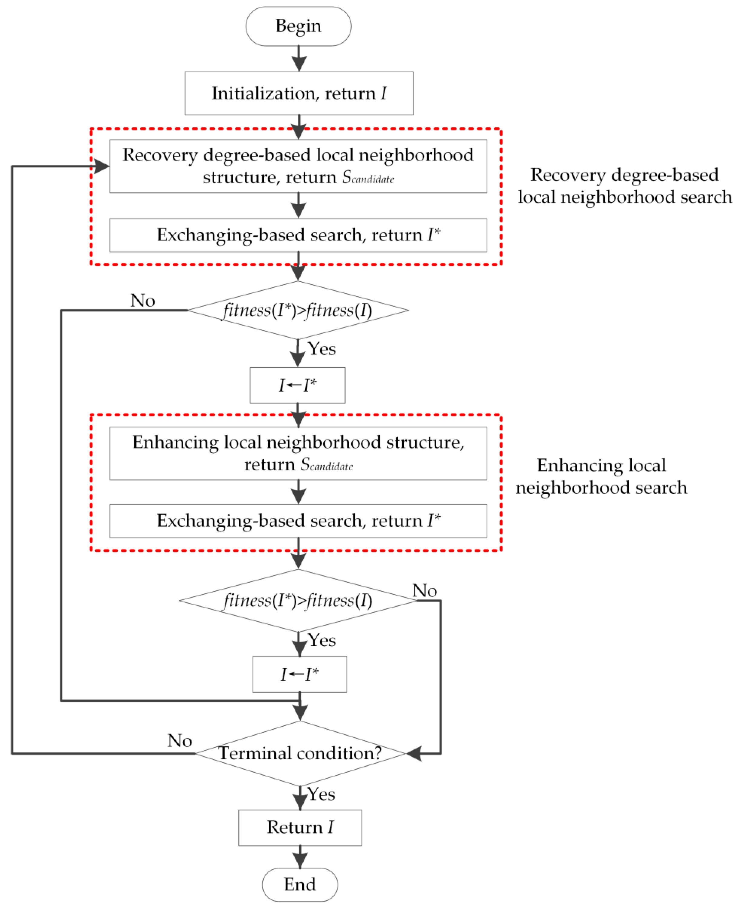
In the EVNS, a two-stage solution improvement procedure is proposed, which is composed of a recovery degree-based local neighborhood search, enhancing local neighborhood search, and secondary optimization-based neighborhood selection scheme.

To evaluate the proposed two-stage solution improvement method, experiments are also conducted to compare the EVNS with three other algorithms, specifically RLNS, ELNS, and EVNS0. In the RLNS, the algorithm only performs the recovery degree-based local neighborhood search. As for ELNS, it will only use the enhancing local neighborhood search to find optimal solutions. In EVNS0, the secondary optimization-based neighborhood selection scheme in the two-stage solution improvement procedure is replaced by random selection. Comparative experiments were performed on two instances, namely recovering 0.6% disrupted suppliers under a random and target disruption of 3000 suppliers respectively. Each algorithm was run 10 times on each instance within the same maximum running time of 60 s.

Figure 12 and

Table 4. Optimal solution fitness comparison of EVNS, RLNS, ELNS, and EVNS0.

	Random Disruption			Target Disruption
	faver	fmax	fmin	faver	fmax	fmin
EVNS	1.8901	1.9054	1.8834	1.2943	1.3341	1.2104
RLNS	1.8454	1.8629	1.8203	1.1879	1.2616	1.1087
ELNS	1.8797	1.9039	1.8621	1.2704	1.2782	1.2561
EVNS0	1.8688	1.8842	1.8408	1.2819	1.3105	1.2522

present the experimental results. Figure 12a,b shows the fitness curve comparisons of the four algorithms under random and target disruption of 3000 suppliers respectively. It can be observed that the EVNS is capable of finding better solutions within a shorter time in both Figure 12a,b. For each instance, the average fitness value, the best fitness value, and the worst fitness value of the 10 trials achieved by each algorithm are also presented in Table 4. It shows that EVNS attains the best results in terms of three indicators for both instances. It can be induced that the proposed two-stage solution improvement is able to improve algorithm performance, suggesting that the EVNS-based recovery supplier selection method can efficiently find these critical disrupted suppliers which are necessary to be recovered as soon as possible.

5.3. Discussion of Experimental Results

Structural characters of the empirical supply network are investigated. The degree distributions of it are highly skewed. One implication of such structural character is that the network can retain its function in the presence of random supplier disruptions. On the other hand, the disruption of hub suppliers with massive product supply edges may damage the function of the overall network significantly.

Comparative experiments verify the effectiveness of the proposed EVNS-based recovery supplier selection method. It is found that the proposed EVNS-based method outperforms other methods under both random and target disruption scenarios. Comparing with target disruptions, the tolerance of random disruptions in the empirical supply network is stronger. This is consistent with the skewed degree distribution. Additionally, under both random and target disruption scenarios, it is observed that recovering very few disrupted suppliers can alleviate the impacts caused by massive supplier disruptions greatly. However, it is also found that along with the increase of recovery suppliers, the recovering rate of both performance metrics also slow down. Thus, it is important to determine a proper number of recovery suppliers in practice.

6. Conclusions

6.1. Contributions to Knowledge

To cope with the various, unavoidable and unpredictable supply network disruptions, it is essential to design proper recovery strategies for a post-disruption supply network, such as recovery supplier selection. Previous studies considered the recovery supplier selection problem from the focal or dyad view [10,11,12,13], without the consideration of the supply network structure. However, today’s supply networks can be huge and complex. Disruption management needs to consider the supply network structure from a macro level [31,32,33]. Thus, this study proposes a recovery supplier selection method from the network structure level to fulfill the knowledge gap. The knowledge contributions are concluded as below.

First, to reflect the heterogeneous roles of manufacturers and suppliers and the various product supply-demand relations between them, a tripartite graph-based supply network model is designed. Unlike many previous studies [21,22,23,31], the proposed model is capable of reflecting the heterogeneous roles of nodes in a supply network. Facilitated by the model, two performance metrics are also proposed to describe product supply availability in the network.

Second, the EVNS-based recovery supplier selection method is proposed. The recovery supplier selection is formulated as a combinatorial problem. To solve the problem effectively and efficiently, a variant of a VNS, the EVNS is proposed. In the algorithm, a two-stage solution improvement is designed to improve the searching efficiency. The effectiveness of it is validated using experiments.

Thirdly, contributions to supply network structural analysis are also made in this work. An empirical supply network is built using the product supply-demand information from the automobile industry. Structural characters of it are investigated. It is found that the degree distributions are highly skewed. That is to say, hub suppliers with massive edges are critically important to the overall network, the disruption of them can reduce the function of the entire network evidently. In the meanwhile, the network can tolerate random supplier disruptions.

6.2. Implications for Practice

The presented method provides a reactive approach for decision-makers, such as supply chain managers or service companies, to build a resilient supply network. The practical applicability of it to alleviate the damages caused by supplier disruptions has already been verified in the case example. This subsection will discuss these practical implications further.

Firstly, the decision-makers can use the proposed supply network model and performance metrics to estimate the damage caused by potential single or supplier disruptions. This can present a robustness assessment of supply networks.

Secondly, the decision-makers can use the proposed method to determine an appropriate response to supplier disruptions. After the selection of recovery suppliers, immediate responses, such as the activation of assistant actions, are required. However, it is also noticed that the recovering speeds of both performance metrics are slowing down with the increase of the number of recovery suppliers. Thus, it is important to determine a proper number of recovery suppliers in practice.

Thirdly, this research also has implications for supplier evaluation and management practices. Usually, companies focus on the internal qualities or capabilities when evaluating suppliers. Structural analysis of the empirical supply network indicates individual suppliers’ structural positions should be paid more attention. Some suppliers occupy the central positions, disruption of them may impact the entire system greatly. For such suppliers, decision-makers should monitor them more closely.

Finally, since the empirical supply network structure shows different robustness to different disruption types, decision-makers may consider designing the supply network in a way that it can retain functionality under various types of disruptions.

6.3. Limitations and Further Work

The following aspects of the research can be extended in the future.

Firstly, considering the visuality of manufacturers is often limited within their first-tier suppliers, the proposed supply network model only considers the interdependence between manufacturers and their directed suppliers. However, knowing the extended network is important, so that appropriate risk mitigation plans can be prepared in advance. We may use the link prediction method to solve the problem of losing visibility of extended networks and expand this research into a multi-tier structure.

Secondly, the cascading failures are neglected in this work. In reality, the disruption can cascade through the supply network, leading to significant economic loss. Since the supply model proposed in this study considers the role differences between manufacturers and suppliers and differentiates the various product supply-demand relations connecting them, the traditional cascading model for unipartite networks can not be applied in the proposed model. We will try to develop appropriate cascading models, which can bring the product supply-demand relations between suppliers and manufacturers together.