On Numerical 2D P Colonies Modelling the Grey Wolf Optimization Algorithm

Abstract

The 2D P colonies is a version of the P colonies with a two-dimensional environment designed for observing the behavior of the community of very simple agents living in the shared environment. Each agent is equipped with a set of programs consisting of a small number of simple rules. These programs allow the agent to act and move in the environment. The 2D P colonies have been shown to be suitable for the simulations of various (not only) multi-agent systems, and natural phenomena, like flash floods. The Grey wolf algorithm is the optimization-based algorithm inspired by social dynamics found in packs of grey wolves and by their ability to create hierarchies, in which every member has a clearly defined role, dynamically. In our previous papers, we extended the 2D P colony by the universal communication device, the blackboard. The blackboard allows for the agents to share various information, e.g., their position or the information about their surroundings. In this paper, we follow our previous research on the numerical 2D P colony with the blackboard. We present the computer simulator of the numerical 2D P colony with the blackboard and the results of the computer simulation, and we compare these results with the original algorithm.

1. Introduction

Membrane systems, P systems, (see [1,2]) are bio-inspired computational systems. The inspiration is taken from living cell membranes, where the computation is provided by letting an object from the environment pass through the membranes of the cell.

Many variants of the P systems were introduced during two decades of research in the field of membrane computing. One of the variants of the P systems is the P colony (see [3,4]). P colony consists of the very simple organisms, the agents, living in the shared environment. The environment of the P colony is a multiset of objects, and each agent is equipped by the set of programs allowing them to handle the objects. Each program consists of rules allowing the agent to exchange one object from the environment for another one inside the agent, or evolve the object inside of them into the other object.

The 2D P colony (see [5]) is a variant of P colonies. The main difference between P colony and the 2D P colony is that the environment of the 2D P colony is given by a matrix, where each cell of the matrix is represented by a multiset of objects. Besides the mentioned rules, the agents of the 2D P colony can use also rules for moving between the cells of the environmental matrix.

The P colonies and 2D P colonies were successfully applied in various fields of computer science. In [6], the P colony was used as a robot controller. In [7], the successful simulation of flash floods was provided by the 2D P colony.

The optimization problem is one of the main issues in computer science. There are many approaches to solving the optimization problem. One of the approaches is represented by the Grey wolf algorithm. The Grey wolf optimization algorithm (GWO) is a meta-heuristic optimization technology. Its principle is to imitate the hunting process of the pack of grey wolves in nature. There are four types of grey wolves used—alpha, beta, delta, and omega—to simulate the hierarchy in the pack. In addition, the three main steps of hunting, searching for prey, encircling prey, and attacking prey, are implemented. The algorithm was introduced by Mirjalili et al. in 2014 in [8].

P systems were successfully used for solving optimization problems. Recently, T. Y. Nishida designed membrane algorithms (see [9]) for solving NP-complete optimization problems, namely the traveling salesman problem (see [10]). G. Zhang, J. Cheng and M. Gheorghe proposed ACOPS, the combination of the P systems with ant colony optimization for solving the traveling salesman problems (see [11]). In [12], the similarities between the distributed evolutionary algorithms and membrane systems for solving continuous optimization problems were studied.

The original model of the 2D P colony cannot successfully simulate the GWO; while the agents are able to communicate only via the environment, they are not able to share their positions, hence they are not able to form the desired hierarchy, and successfully hunt down the prey. Moreover, the environment of the 2D P colony is a multiset of objects. In [13,14,15], we introduced a numerical version of the 2D P colony equipped by the blackboard, where the discrete values of the fitness function represents the environment. These modifications of the 2D P colony were designed for the simulation of the Grey wolf algorithm. In this paper, we present the computer simulator of the extended version of the 2D P colony, and the results obtained during the simulations.

2. Numerical 2D P Colony with a Blackboard

Let us remind the formal definition of the numerical 2D P colony with a blackboard first (see [13,14]).

Definition 1.

A numerical 2D P colony with blackboard is a construct

$$\mathrm{\Pi }=(V,e,Env,A_1,\dots ,A_k,BB,f),k\ge 1,where$$

• V is the alphabet of the colony. The elements of the alphabet are called objects. $\square$ are special objects, that can contain an arbitrary number.
• $e\in V$ is the basic environmental object of the numerical 2D P colony,
• $Env$ is a triplet $(m\times n,w_E,f_E)$, where $m\times n,m,n\in N$ is the size of the environment. $w_E$ is the initial contents of the environment, it is a matrix of size $m\times n$ of multisets of objects over $V-\left\{e\right\}\cup \left\{f_E\left(x\right)\right\}$. $f_E$ is an environmental function. The environmental function represents the optimization problem, hence the domain and range are given by the definition of the problem.
• $A_i,1\le i\le k$, are the agents. Each agent is a construct $A_i=\left(o_i,P_i,[o,p]\right),$$0\le o\le m,0\le p\le n$, where

  –

  $o_i$ is a multiset over V, it determines the initial state (contents) of the agent, $|o_i|=2$,

  –

  $P_i=\left\{p_{i,1},\dots ,p_{i,l_i}\right\},l\ge 1,1\le i\le k$ is a finite set of programs, where each program contains exactly 2 rules. Each rule is in the following form:

  *

  $a\to b$, the evolution rule, $a,b\in V$,

  *

  $c\leftrightarrow d$, the communication rule, $c,d\in V$,

  *

  $\left[a_{q,r}\right]\to s,a_{q,r}\in V,0\le q,r\le 2,s\in \{\Leftarrow ,\Rightarrow ,\Uparrow ,\Downarrow \}$, the motion rule,

  *

  $a\rightarrowtail \boxed{x}$, $x\in \mathbb{R},a,\boxed{x}\in V,$ is the communication rule to read the numbers from the environment.

  If the program contains evolution or communication rule $r_1,r_2$ that each works with objects with numbers, it can be extended by a condition: $〈x>y:r_1,r_2〉,$$〈x\ge y:r_1,r_2〉,$

  –

  $[o,p],0\le o\le m,0\le p\le n,$ is an initial position of agent $A_i$ in the 2D environment,

• $BB$ is the blackboard—the blackboard is, in general, a matrix-like structure, which is accessible for all the agents for storing and obtaining the information. The structure of the blackboard is given by the definition of the particular P colony. The communication between the blackboard and agents is ensured by the functions $\mathit{Get}$ and Update.
• $f\in V$ is the final object of the colony.

A configuration of the numerical 2D P colony with the blackboard is given by the state of the environment—matrix of type $m\times n$ with pairs—multiset of objects over $V-\left\{e\right\}$, and a number—as its elements, and by the states of all agents—pairs of objects from the alphabet V, and the coordinates of the agents. An initial configuration is given by the definition of the numerical 2D P colony with the blackboard.

The environment of the numerical 2D P colony is, in general, given by the matrix. Each element of the matrix is represented by the multiset of objects over the alphabet $V-\left\{e\right\}$ and it also contains the value of the environmental function, a real number in general. The values of the environmental function form the three-dimensional graph of the function.

A computational step consists of three steps. In the first step, the set of the applicable programs is determined according to the current configuration of the numerical 2D P colony with the blackboard. In the second step, one program from the set is chosen for each agent, in such a way that there is no collision between the communication rules belonging to different programs. In the third step, chosen programs are executed, the values of the environment and on the blackboard are updated. If more agents execute programs to update the same part of the blackboard, only one agent is non-deterministically chosen in order to update the information. The agent has no information if his attempt to update the blackboard was successful or not.

A change of the configuration is triggered by the execution of programs, and updating values by functions. It involves changing the state of the environment, contents and placement of the agents.

A computation is non-deterministic and maximally parallel. The computation ends by halting, when there is no agent that has an applicable program.

The result of the computation is the number of copies of the final object placed in the environment at the end of the computation.

3. Grey Wolf Optimization Algorithm

Let us also recall basic features of the Grey wolf optimization algorithm (GWO) (see [8,16]). The grey wolves create a social hierarchy in which every member has a clearly defined role. Each wolf can fulfill one of the following roles:

• Alpha pair is the dominant pair and the pack follows their lead.
• Beta wolves support and respect the Alpha pair during its decisions.
• Delta wolves are subservient to Alpha and Beta wolves, follow their orders, and control Omega wolves. Delta wolves divide into scouts—they observe the surrounding area and warn the pack if necessary, sentinels—they protect the pack when endangered, and caretakers—they provide aid to old and sick wolves.
• Omega wolves help to filter the aggression of the pack and frustrations by serving as scapegoats.

The primary goal of the wolves is to find and hunt down prey in their environments. The hunting technique can be divided into five steps:

• Search for the prey
• The exploitation of the prey
• Encircling prey
• The prey is surrounded
• The attack

The GWO algorithm is inspired by this process and smooth transitions between scouting and hunting phases. The prey represents the optimal solution to the given problem, and the environment is represented by a mathematical fitness function that characterizes this problem. The value of the function at the current position of the particular wolf represents the highest-quality prey. The wolf with the best value is ranked as Alpha, the second one as Beta, third as Delta, and all the others are Omegas.

In the scouting phase, the pack extensively scouts its environment through many random movements, so that the algorithm does not get stuck in a local extremum, while in the hunting phase, the influence of random movements is slowly reduced and pack members draw progressively closer to the discovered extremum.

4. The Analysis of the System

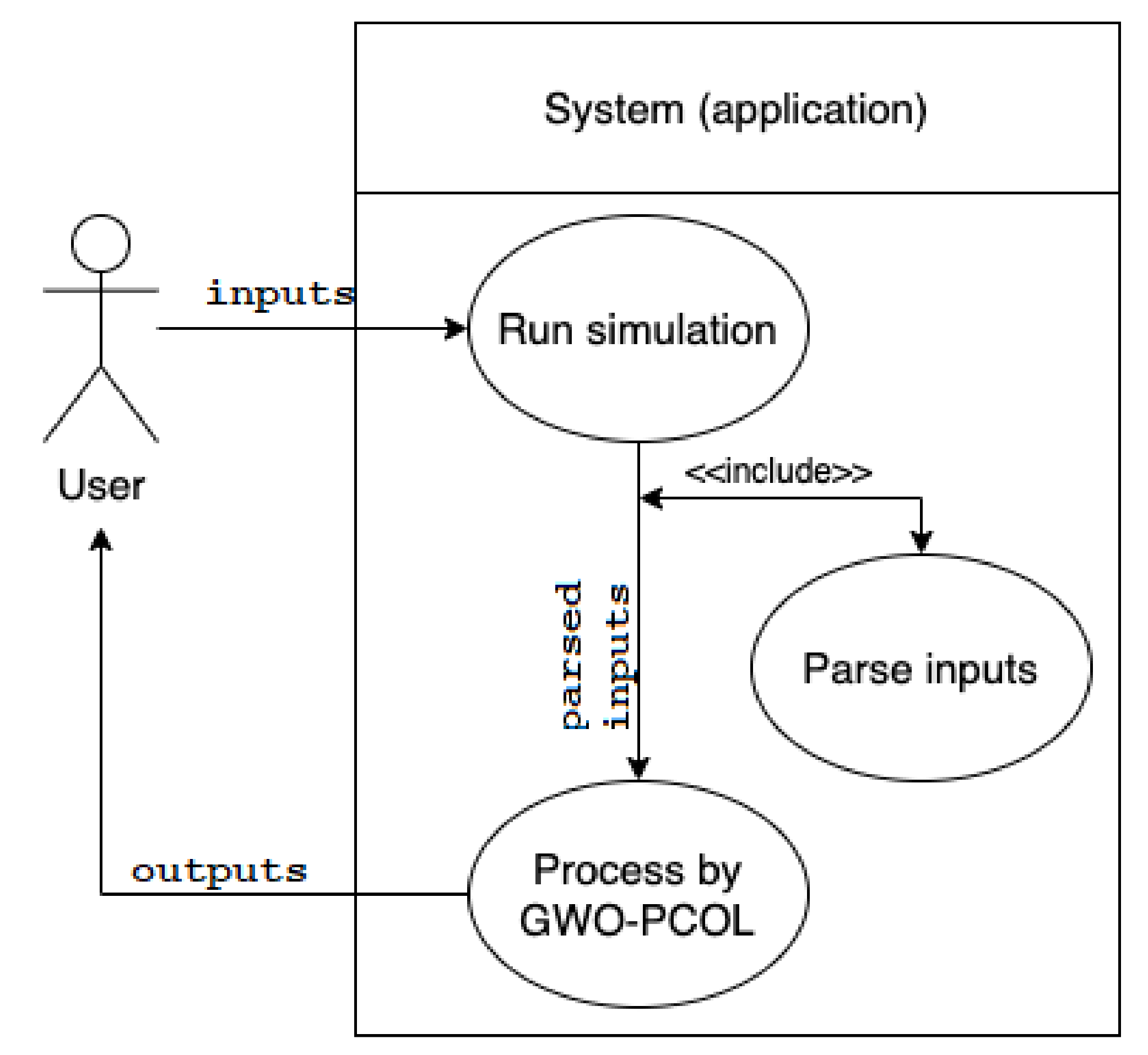
First, we provide a general analysis of the application. The use case diagram presented in Figure 1 gives us a clear overview of the basic functions that are provided by the application. The single-user application allows us to run the simulation of the GWO algorithm, simulated by the 2D P colony based on the inputs given by the user.

The inputs of the application are:

• the environment,
• GWO inputs,
• the rules of the agents.

The user (without the programmer’s knowledge) can edit each of the inputs. The application provides the following user functionalities:

• simulation, including the information about the configuration of the agents and the blackboard, and allows to follow each derivation step of each agent, and
• visualization of the simulation, a graphical representation of the environment, blackboard, and the agents, visualization of the model behavior in each step.

The application provides the console output for a full overview of the information about the status of the system during the simulation, and the graphical interface used for the visualization of the simulation.

5. The Inputs of the Algorithm

The inputs of the algorithm are a crucial part of the application. The inputs must be in the given structure; otherwise, the parser will not be able to parse and read the input data. In the following sections, we will describe particular inputs, their parsing process, and we will also give examples of the particular data.

5.1. The Environment

In general, the environment of the 2D P colony is a matrix of multisets. For the purpose of the simulation, we use matrix of integers only.

The representation of the environment is implemented as a matrix of size $m\times n$. The matrix is saved in the text file having the following structure:

• each element of the matrix is represented by a float number,
• the numbers (columns) are separated by the space (“ ”),
• the rows of the matrix are separated by a new line (“$\setminus n$”), and
• the matrix must have the same number of elements in each line.

Let us focus on an example. Let the matrix A defines an environment:

$$A=\left(\begin{array}{cc}1& 2\\ 3& 4\\ 5& 6\end{array}\right)$$

(1)

The only structure of the A the algorithm accepts is the following text file:

$$\begin{array}{cc}1& 2\\ 3& 4\\ 5& 6\end{array}$$

(2)

The file containing the environment has an extension “env”.

The environment parser is very simple. The parsing algorithm uses two nested for loops to access each of the elements from the input file (see Algorithm 1).

The structure of the loaded file is an array. Attributes NumberOfLines and NumberOfColumns define the number of rows and columns in this array, and they are obtained while using the function np.shape (see [17]) from the loaded env file.

Each of the elements stored in the file is checked during the parsing phase. The file is successfully parsed only if all of the elements are of the float type, and the number of elements is the same in each line. Otherwise, a syntax error occurs.

After the parsing phase, the stored elements are drawn into the graphical interface of the application.

As an example, we show a fitness function $F=-\left(x^2+y^2\right);x,y\in \left(-5,5\right)$. The plot of the function is in Figure 2.

The following matrix represents this function in the form acceptable by the algorithm.

Algorithm 1: Parsing the environment

$Environment=\left[\right]\left[\right]$

for $x\in range(0,NumberOfLines)$ do

for $y\in range(0,NumberOfColumns)$ do

$Environment\left[x\right]\left[y\right]\leftarrow Element(x,y)$

end for

end for

$$\begin{array}{ccccccccccc}75& 84& 91& 96& 99& 100& 99& 96& 91& 84& 75\\ 94& 103& 110& 115& 118& 119& 118& 115& 110& 103& 94\\ 111& 120& 127& 132& 135& 136& 135& 132& 127& 120& 111\\ 126& 135& 142& 147& 150& 151& 150& 147& 142& 135& 126\\ 139& 148& 155& 160& 163& 164& 163& 160& 155& 148& 139\\ 150& 159& 166& 171& 174& 175& 174& 171& 166& 159& 150\\ 159& 168& 175& 180& 183& 184& 183& 180& 175& 168& 159\\ 166& 175& 182& 187& 190& 191& 190& 187& 182& 175& 166\\ 171& 180& 187& 192& 195& 196& 195& 192& 187& 180& 171\\ 174& 183& 190& 195& 198& 199& 198& 195& 190& 183& 174\\ 175& 184& 191& 196& 199& 200& 199& 196& 191& 184& 175\\ 174& 183& 190& 195& 198& 199& 198& 195& 190& 183& 174\\ 171& 180& 187& 192& 195& 196& 195& 192& 187& 180& 171\\ 166& 175& 182& 187& 190& 191& 190& 187& 182& 175& 166\\ 159& 168& 175& 180& 183& 184& 183& 180& 175& 168& 159\\ 150& 159& 166& 171& 174& 175& 174& 171& 166& 159& 150\\ 139& 148& 155& 160& 163& 164& 163& 160& 155& 148& 139\\ 126& 135& 142& 147& 150& 151& 150& 147& 142& 135& 126\\ 111& 120& 127& 132& 135& 136& 135& 132& 127& 120& 111\\ 94& 103& 110& 115& 118& 119& 118& 115& 110& 103& 94\\ 75& 84& 91& 96& 99& 100& 99& 96& 91& 84& 75\end{array}$$

(3)

5.2. The Rules of the Agents

The Rules of the Agents can be defined by the user in an XLS (MS Excel) file. The file has the following structure. The first line describes the columns of the file. This line is for the user to orientate in the file only, and it does not affect the algorithm. The following lines define the rules. An example of the definition of the rules is in the

Table 1. The structure of the file of the rules of the agents.

State	X	Y	Try	Else
The state of the rule	The first object of the agent	The second object of the agent	[Actions]	[Alternative actions]

.

Each rule consists of five attributes:

• The state of the rule—a positive integer value defines the state of the rule. The initial value of the state equals 0. In the Actions or Alternative actions, the state of the rule can be changed to a different value. In such a case, the agent provides more actions in one iteration step. The next iteration, the synchronization of the agents, starts when the state is set back to 0. This also means that the rule was applied successfully.
• The first and the second objects of the agent—the configuration of the agent—the objects inside the agent represented by the characters.
• [actions]—a sequence of the actions to be run if the previous conditions are fulfilled (the state of the rule and configuration of the agent).
• [alternative actions]—a sequence of the alternative actions to be run if any of the actions fail.

Let us focus on the possible values in particular cells:

• The state of the rule (column State) $=\{S,S\in \mathbb{N}\}$, agents are synchronized if $S=0$ (rule was applied successfully)
• The first object of the agent (column X) $=\{x,x\in \{a,\dots ,z,A,\dots ,Z\}\cup int\}$, where $int$ is the keyword that represents any number from the $\mathbb{Z}$.
• The second object of the agent (column Y) $=\{y,y\in \{a,\cdots ,z,A,\cdots ,Z\}\cup >=\}$, where $>=$ is the keyword to compare the first and second objects of the agent–the assumption is that $X,Y\in \mathbb{Z}$.
• [Actions] (column Try) and [Alternative actions] (column Else) contain the keywords that are separated by space:

  –

  $x=i$, and $y=j$, are the keywords for updating objects X or Y inside the agents, where: $i,j\in \{a,\cdots ,z,A,\cdots ,Z\}\cup \{env,BB[i],Rand(g\left)\right(h\left)\right\}$. The keyword $env$ activates the function getting int value from the environment, and $BB\left[i\right]$; $i=A,B,D$, is the keyword activating the function obtaining the value from the blackboard at the position i $(A=Alpha,B=Beta,D=Delta)$. $Rand\left(g\right)\left(h\right)$ is the keyword that activates the function generating random value in the range from g to h.

  –

  $state=n,n\in S$, is the keyword that changes the state of the rule.

  –

  $Update\left(BB\right[i\left]\right);i=A,B,D$, is a keyword that activates the function updating value on the blackboard at position i$(Alpha,Beta,Delta)$.

  –

  $Move\left(q\right),q=\{L,R,U,D\}$ or $\{1,2,3,4\}$, is the keyword activating the function moving the agent, where $L=1=Left,R=2=Right,U=3=Up,D=4=Down$.

  –

  $AssistMove\left(\right)$ is the keyword that activates the function moving the agent with an assistance of the blackboard, i.e., all directions will be tried.

  –

  $death\left(\right)$ is the keyword terminating the activity of the agent.

  –

  $Index\left(a\right)$ is the keyword that returns true if the index of the agent equals a.

The parser for the rules of the agents file is implemented in the very same way as the parser of the files of the environment. The algorithm uses two nested for loops to read each of the elements from the input (.xls) file (see Algorithm 2).

Algorithm 2: Reading the rules

for $Agentsinstate0$ do

if $X==\left[Firstobjectoftheagent\right]\mathbf{and}Y==\left[Secondobjectoftheagent\right]$ then

$\mathbf{Try}:do\left[Actions\right]$

$\mathbf{Else}:do\left[Alternateactions\right]$

end if

end for

In case that the applied action (or alternative action) changes the state of the rule to the value higher than 0 (by the action “state=n”), the rules of the same value of the state are being executed, until the rules of all agents are in state 0 again.

We give two examples of the definitions of the rules.

The set of rules in

Table 2. GWO-2D P colony model, the definition of the rules.

State	X	Y	Try	Else
0	e	e	X=env Y=BB[A]
0	int	$>=$	Y=A	Y=BB[B] state=1
0	int	A	Update(BB[A]) X=e Y=e
1	int	$>=$	Y=B state=0	Y=BB[D] state=2
2	int	$>=$	Y=D state=0	Y=BB[i] Y=O state=0
0	int	B	Update(BB[B]) X=e Y=e
0	int	D	Update(BB[D]) X=e Y=e
0	int	O	AssistMove() X=e Y=e	X=f Y=f
0	f	f	death()	X=e Y=e

defines the simulation of the Grey wolf optimization algorithm using 2D P colonies. Note the use of the space character (“ ”) as a separator between each action in the Try and Else columns. The states 1 and 2 in the 4. and 5. line are used to give an example of the more complex rule that compares up to three values—the agents are not synchronized until all of their rules are in the state 0.

The set of rules defined in

Table 3. A simple swarm optimization algorithm, the definition of the rules.

State	X	Y	Try	Else
0	e	e	Index(0) state=1	state=2
1	e	e	X=Rand(1)(4) Y=m
1	int	m	Move(X) Y=u
1	int	u	Update(BB[A]) X=e Y=e state=0
2	e	e	X=BB[A] Y=m
2	int	m	Move(X) X=r Y=r
2	r	r	X=e Y=e state=0

defines the simulation model of a simple swarm optimization algorithm. One of the agents–agent with index 0 is the so-called leader. The leader sends information about its movements to the blackboard, and the other agents repeat it with a delay of one step. In this model, the fitness values are not important, they do not affect the movements of the agents in any way.

One must keep in mind that, if the rule is composed of several states, there must always be a path back to state 0.

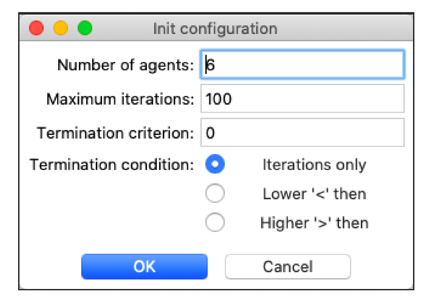
5.3. Input Arguments for GWO

The original Grey wolf optimization algorithm expects the arguments that are described in

Table 4. GWO input arguments.

Input Argument	Preset Value
Population size (number of wolves)	6 (typical number of wolves in a pack)
Comparison operator for Fitness function (smaller than or greater than)	>(finding the maximum)
Termination criterion	100 iterations

as its input.

In the application, the users can modify these values in a dialogue window before running the simulation, as it can be seen in Figure 3.

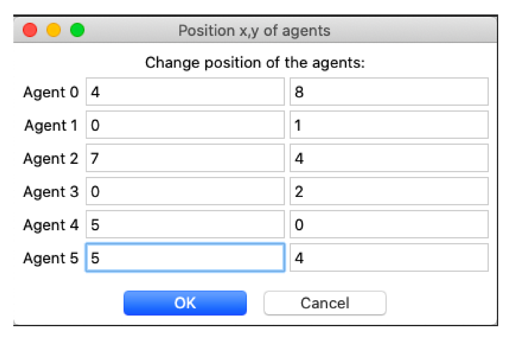
The user can also modify the initial positions of the agents in the environment, as it can be seen in Figure 4. It is useful to verify the correct location of the agents, in the case of specific requirements, like testing the desired behavior.

6. The Components of the Application

In this section, we present individual components of the algorithm. These components can be sensed as the classes or object, respectively. There are three main components:

• the agent,
• the configuration of the system, and
• and the blackboard.

6.1. The Agent

Each agent is implemented as an object of the class Agent and it is defined by the following set of attributes. The attributes forms the configuration of the agent:

• index—the index, pointer of the agent,
• pos—the position of the agent in the environment—X and Y coordinates,
• obj1 and obj2—two objects inside the agent, and
• ruleState—the state of the rule.

The activity of the agent is provided by executing the rules matching the configuration of the agent. Each rule causes an activation of one of the following methods:

• AgentSymUpdate—evolving the objects inside the agent,
• MoveAgent—moving the agent in desired direction (left, right, up, or down),
• AssistMove—moving the agent with the assistance of the blackboard.

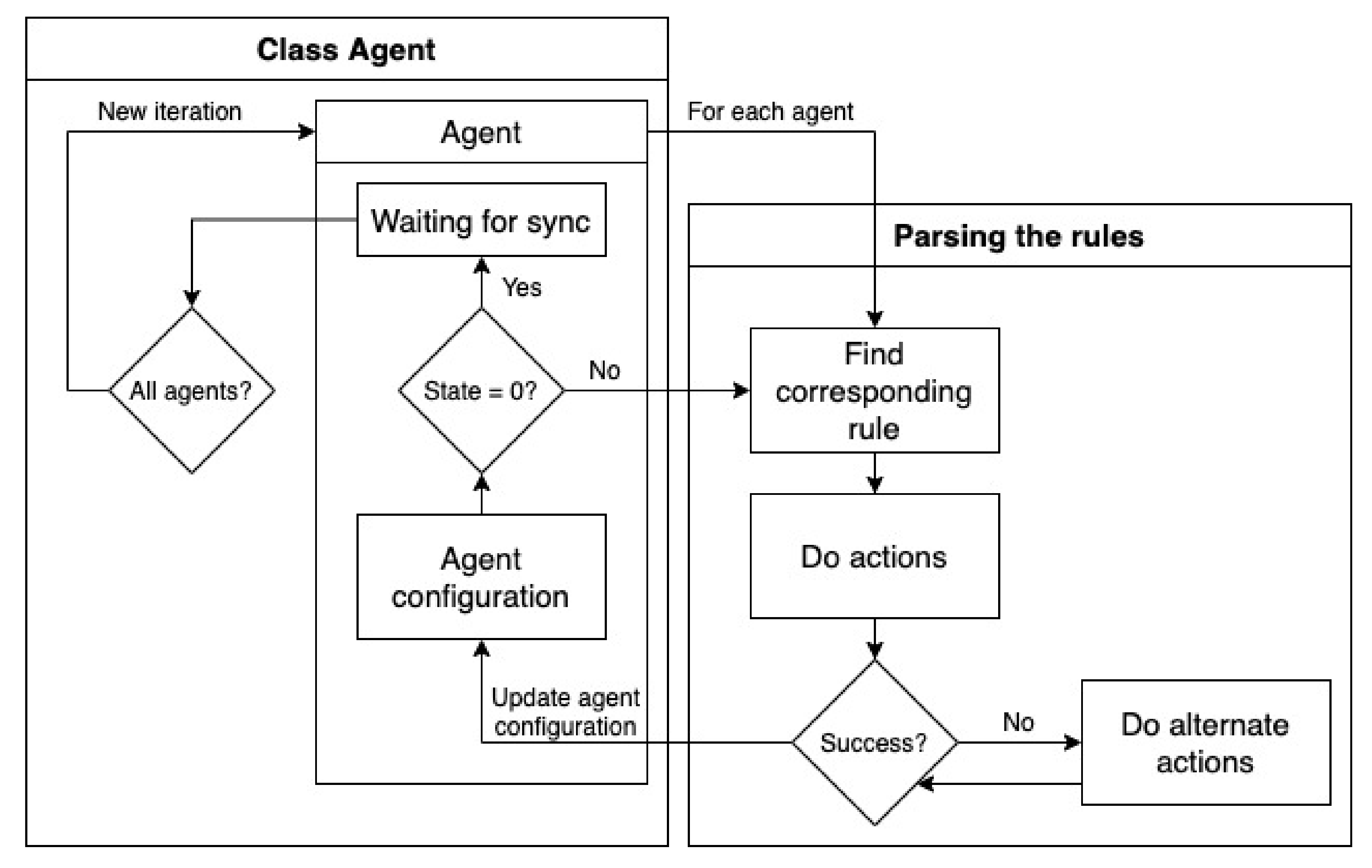
Figure 5 shows the flowchart of the algorithm controlling the behavior of the agents. The algorithm can be divided into the following blocks:

• start of a iteration—selecting the applicable rule,
• execution of the rule(s), and applying the changes to the environment, and
• update of the blackboard.

First, the applicable rule is found for each agent. The rule is chosen on the dependence on the recent configuration of the agent. This step can only be executed only if the parameter $State=0$, which means that the agents are synchronized (no agent is executing any of its rules) and a new iteration starts. One iteration of the agent can consist of several steps. This happens when the value of the $State$ is set to the value greater than 0 by some [Actions] or [Alternative actions]. The algorithm continues by finding another rule with the same value of the $State$. If the value of the parameter $State$ equals 0, the rule is applied, and the agent changes its state to Waiting for synchronization before a new iteration.

Let us focus on the difference between the step and the iteration now. First, the iteration can be composed of several steps. In a step, the actions (or alternative actions) of each of the agents that are not waiting for synchronization are applied. Changes to the environment are made at the end of this step. If there is at least one rule having parameter $State$ greater than 0, the next step is provided. The new iteration begins when every agent is waiting for synchronization, hence every agent has completed a rule, changed its configuration, and the parameter $State$ parameter is zero.

At the beginning of a new iteration, the blackboard is updated and the termination criterion is checked.

The Configuration of the System Information

The output console (see section Graphical interface, Section 8) displays information regarding the recent configuration of the system, i.e., the configurations of the agents, information about applied rules, used actions, and derivation steps. The configuration is displayed in the plain text. The

Table 5. State information of the agents.

State Information	Description
Time of last n step(s)	Information about the time in total taken by the simulation.
Agent i configuration: position: ($PosX$, $PosY$); object1 = X; object2 = Y	Information about the current configuration of the agent.
Agent i is now waiting for synchronization.	Information, that the $i-th$ agent is waiting for the synchronization.
Agent i wants to be [$Alpha$, $Beta$, $Delta$]	Information that the $i-th$ concluded it is Alpha/Beta/Delta.
Agent i found the rule just for him.	$i-th$ agent has found an applicable rule.
No rule for this configuration! X, Y	Information about the missing rule for some configuration.
[Actions, Alternate actions] completed successfully. Configuration of $i-th$ agent changed.	$i-th$ agent successfully finished all the actions in the particular iteration and changed its configuration according to the applied rules.
Agent i is trying to move	$i-th$ agent is trying to move without the assistance of the blackboard.
Agent i is trying to move with BB assistance	$i-th$ agent is trying to move with the assistance of the blackboard.
No agent i movement.	$i-th$ agent is remaining in its position.

describes information given in the console.

Table 5 uses the following symbols:

• i is the index of the agent,
• n is the user defined number of the steps,
• X, Y are the objects inside the agent, and
• $PosX$, $PosY$ are the coordinates of the agent.

6.2. The Blackboard

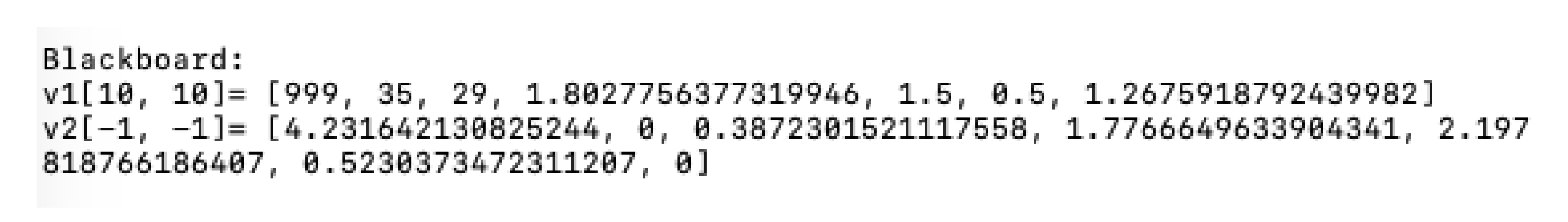
The blackboard is implemented as a structure of two arrays of size equal to a number of wolves. The minimal size of vector $v_1$ is 7 (six fields are reserved for $Alpha$, $Beta$, $Delta$, and 1 for the position of prey). The application displays the blackboard in the following form:

$$v_1[r_1,r_2]=[AlphaValue,BetaValue,DeltaValue,AlphaDistance,BetaDistance,$$

$$DeltaDistance,PreyPosition],$$

$$v_2[s_1,s_2]=[A_{1}DistanceFromPrey,A_{2}DistanceFromPrey,\dots ,A_{n}DistanceFromPrey],$$

where $v_1$, $v_2$ are the vectors, $r_1$, $r_2$ are coordinates of the first receiver, and $s_1$, $s_2$ are coordinates of the second receiver.

In Figure 6, the visualization of the blackboard in the application is shown. We have defined the following methods for manipulating these arrays:

• $Update\left(\right)$—method updating the values reserved for Alpha, Beta, or Delta wolves,
• $Get\left(\right)$—method reading the values from arrays, and
• $Newiteration\left(\right)$—method calculating a new position of the prey and the distances of wolves from the prey.

The communication between the agent and the blackboard is implemented by the method of blackboard, called Message. This method expects the following arguments: function ($0=Get$, $1=Update$), function argument (for example value to update), the index of the agent, and sender (agent) position in the environment).

For example, a message $Message(0,0,self.index,pos)$ means, that the agent with $self.index$, at position $pos$, is trying to use function $Get\left(0\right)$.

In the model that was introduced in [14], two receivers are listening to the signals (messages) from the agents. The receivers play important role. They calculate the distances of agents from the blackboard (receivers). The distance of the agent is computed as an intersection of the circles $R_1$ and $R_2$, with center at the position of the receivers, and $r=now-sent$, where $now$ is a time of receiving the message, and $sent$ equals to $timestamp$, x is randomly chosen in the intersected area. The shapes of the intersection change during the time due to the movements of the receivers—they rotate around the environment, initial position of the first receiver is $(0,0)$, and of the second receiver $(i,j)$, where i and j are given by the size (dimensions) of the environment.

When compared to the previously presented model, the implementation is a bit different. Receivers are used to approximate the calculation of the agent distance from the blackboard only. Instead of time, rounded positions of the agents and exact positions of the receivers are used. Thanks to this change, the implementation is simpler and it does not affect the functionality of the model. Theoretically, receivers can be replaced by the simple random value, but they are preserved with respect to the model.

The functions of the blackboard $Get$ and $Update$ can be used by the agents and they are activated in the action part of the rule. For example, the action $Update\left(BB\right[A\left]\right)$ updates the first value of the vector $v_1$ ($AlphaValue$). In the same way, $Update\left(BB\right[B\left]\right)$ updates the second value of the vector $v_1$ ($BetaValue$), and $Update\left(BB\right[D\left]\right)$ updates the third value of the vector $v_1$($BetaValue$).

The action of the rule $X=BB\left[A\right]$ or $Y=BB\left[A\right]$ serves to get the first value of the vector $v_1$ ($Alphavalue$) and store it into X (first object of the agent) or Y (second object of the agent). In the same way, other values B and D ($BetaValue$ and $DeltaValue$) can be obtained.

The values $A_{1}DistanceFromPrey$, $A_{2}DistanceFromPrey$, and $A_{3}DistanceFromPrey$ depend on the distance of the agent from the receivers. These values are updated at the same time as the values $AlphaValue$, $BetaValue$, or $DeltaValue$, and they are changed while using the $Get$ function.

The Value $PreyPosition$ of the vector $v_1$ is an auxiliary variable for computing the values of the vector $v_2$, and the agent cannot read or overwrite it. This value is computed at the beginning of each iteration by applying the following formula:

$$PreyPosition=\frac{AlphaDistance+BetaDistance+DeltaDistance3}{3}.$$

Function $Get\left(i\right)$, where i is the index of an agent, can be used to obtain a value from vector $v_2$. This value depends on the distance of the agent from the prey, and it is computed according to the following formula:

$$A_{i}DistanceFromPrey=A_{i}Distance-PreyPosition,$$

where $A_{i}Distance$ value is obtained in the same way as values $AlphaDistance$, $BetaDistance$, and $DeltaDistance$ (thanks to receivers). The action of the rule $AssistMove\left(\right)$ causes the $Get\left(i\right)$ function to be used multiple times. Firstly, to determine the distance of the agent from prey in the current position in the environment, and then in the new positions in order to determine which position is better.

In summary, during an iteration, the blackboard is collecting data from the agents. The value $PreyPosition$ of the vector $v_1$, and the positions of the receivers are updated at the beginning of a new iteration. The values of the vector $v_2$ are updated in real-time (only if the agents request it), and the value depends on the $PreyPosition$ value at the current iteration.

7. The Description of the Algorithm

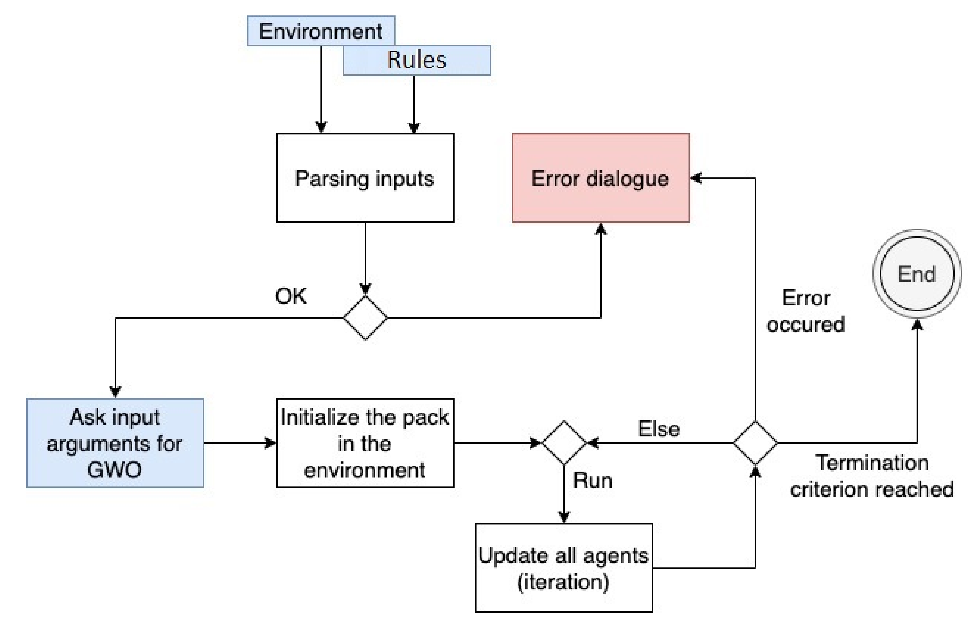
Figure 7 shows the flowchart diagram of the algorithm. It is a diagram of the full process of the algorithm.

First, the input files are parsed. During the parsing process, the syntax of the input is verified. The file containing the rules of the agents "$rules.xls$" is expected in the application directory and it is automatically loaded after the start of the application. The environmental file must be manually chosen by the user from the application menu (Figure 8).

If the inputs are parsed successfully, the simulation can be initialized. During this phase, the user can specify the input arguments that are related to GWO. Subsequently, the agents (pack of wolves) are initialized and placed into the environment.

At this point, the simulation can start. From now on, the user can control the simulation, as it is described in the following section. Before each iteration, the termination criterion is checked. In each iteration, each agent must apply at least one rule. During the runtime, the semantics of the rules are checked. If an error occurs while applying the rules, e.g., an unknown keyword or an unexpected value occurs in a rule, the agent ignores it, i.e., it takes no action, and the user obtains the error message in the console output. The errors are continuously captured and, if a critical error occurs, the application will be terminated.

Table A1. Error messages.

Message	When It Happens	Relevance
File rules.xls cannot be found.	At the star of the application, in the parsing phase	Critical error, the application will be stopped
Invalid environment input file	Loading of environment file, invalid file extension or syntax error	Minor error, a file dialog to select .env file can be opened again
Invalid index in message to Blackboard: [index value]	During the simulation, the customs rule uses the keyword $BB\left[X\right]$ has invalid index X	Minor error, simulation continues, the rule is ignored
Unknown content of the message to Blackboard: [content value]	During the simulation, the agent is trying to use unknown blackboard action - out of range (0=$Get$, 1=$Update$)	Minor error, simulation continues, the rule is ignored
1 argument ’i’ should be used in keyword BB[i]	During the action get value from the blackboard, the number i (arguments) must be equal to 1	Minor error, simulation continues, the rule is ignored
2 argument ’i’, ’j’ should be used in keyword rand(i)(j).	During action generate random value, missing argument in i or j, or too much arguments in i or j.	Minor error, simulation continues, the rule is ignored
Unknown direction to move the agent. Check rules.	During action move the agent, the argument value x in rule Move(x) must be in range 1–4	Minor error, simulation continues, the rule is ignored
Rule state must be integer.	During action change the state of the rule, argument n in rule $State=n$ must be an integer.	Minor error, simulation continues, the rule is ignored
Blackboard cannot be updated by the agent	During the update of the blackboard, agent refers to unknown index of the blackboard	Minor error, simulation continues, the rule is ignored
[Invalid, Unknown ] keyword in rule	Parsing the rule, semantics validation, a rule contains unknown or invalid keyword	Minor error, simulation continues, the rule is ignored
’Number of agents’ value must be in range (1, 99).	In the dialog window, before the agent are initialized	Minor error, the user is asked to change this value
’Maximum iteration’ value must be in range (1, 1000)!	In the dialog window, before the agent are initialized	Minor error, the user is asked to change this value
Integer values are allowed only.	In the dialog window, before the agent are initialized	Minor error, the user is asked to change this value
’Step length’ value must be in range (1, 15)!	After Step button was clicked	Minor error, value in text field set step length must be changed to range 1–15
’Step length’ value must be integer!	After Step button was clicked	Minor error, value in the field set step length must be changed to integer

and

Table A2. Informative messages.

Message	When It Happens	Relevance
Receivers updated: rcv1 = [its position], rcv2 = [its position]	At the beginning of a new iteration	Information about the new positions of the receivers
Rendered simulation opened in a new window.	After using function Draw simulation from the menu	The rendered simulation will be opened in a new window
Console will be redirected to a new window.	After using function Show console from the menu	The console output will be redirected to a new window
Optimal solution found! Best value found: [value]	During the simulation, after running a predefined number of iterations	The termination criterion has been reached
Optimal solution still not found! Best value found: [value]	During simulation, after running a predefined number of iterations	The termination criterion still has not been reached
No termination criterion was specified. Criterion check will be skipped.	During simulation, after running a predefined number of iterations	Informative message about the termination criterion will be skipped, because termination condition was not specified.
Blackboard: [vectors v1 and v2]	At the end of each iteration	Information about the new blackboard updates.
___ITERATION I___	At the beginning of a new iteration	The iteration I starts.
Time of last x steps: t seconds.	After the predefined number of steps	Information about how much time (t) in seconds predefined number of steps (x) took.
Agents initializes to positions: [positions]	After the agents are placed into the environment	Information about the position of the agents in the environment

in Appendix B present an overview of error and info messages, related to the state of the application.

The behavior of the application is strictly dependent on the defined rules. Here we present the pseudocode followed by the model using the rules specified in Table 2:

• in each iteration
  • calculate the value of the fitness function (get the environment value) of each agent and determine the social hierarchy (compare it to Alpha, Beta, and Delta value from the blackboard). The agent with the best value (closest to the optimum) is the Alpha, the second-best is the Beta, the third-best is the Delta, and all others are Omegas (update blackboard),
  • calculate the best solution found so far by Alpha, Beta, and Delta wolves from the blackboard receivers, and then average it,
  • update the positions of all the agents (apply AssistMove rule),
  • check the termination criterion, and
  • the computation stops when the value of the fitness function reaches the preset value.

8. Graphic Interface

Figure 9 displays the main window of the application GUI. The GUI contains the following elements described in separate subsections:

• application menu (highlighted in red),
• canvas displaying the simulation (in orange rectangle),
• buttons controlling the simulation (in blue rectangle),
• text field for the blackboard (in purple rectangle), and
• horizontal and vertical scrollbars (in green rectangle).

8.1. Application Menu

The applications menu is in the toolbar, on the top panel of the screen. It contains three items. The submenus of the items open by clicking on the particular item (Figure 10). Let us describe the items of the menu and their functionalities:

• Environment—allows user to load the environment file:

  –

  Load environment—opens the file dialog window, where the user can select and load the environment file, creates the environment from the loaded environment file.

• Simulation—contains a submenu for managing the simulation:

  –

  Initialization—opens the dialog window with GWO attributes settings. After settings the attributes, agents are initialized and placed into the environment. This item is active before the simulation starts only.

  –

  Draw simulation—opens a new window visualizing the history of agent movements.

  –

  Console output—the console output will be redirected to the new text field window.

• Quit—contains the item to quit the application.

  –

  Quit application—quits the application, including the active simulation.

8.2. Canvas Displaying the Simulation

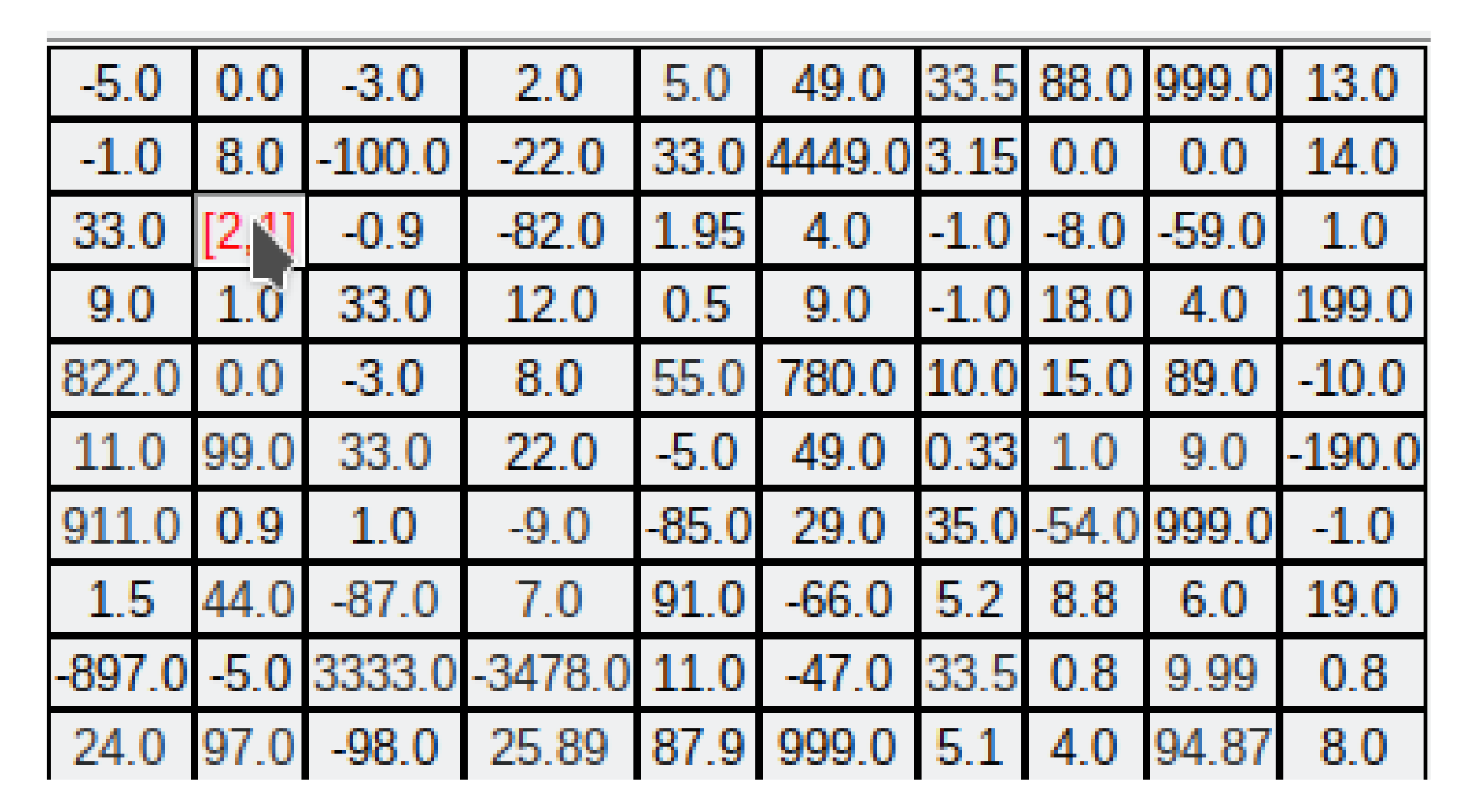
Canvas displaying the simulation is visible only if the environment is loaded. The example in Figure 11 displays the canvas with the loaded instance of the environment. If the user moves the mouse cursor to some field, then they obtain the coordinates of it highlighted by the red color of the text.

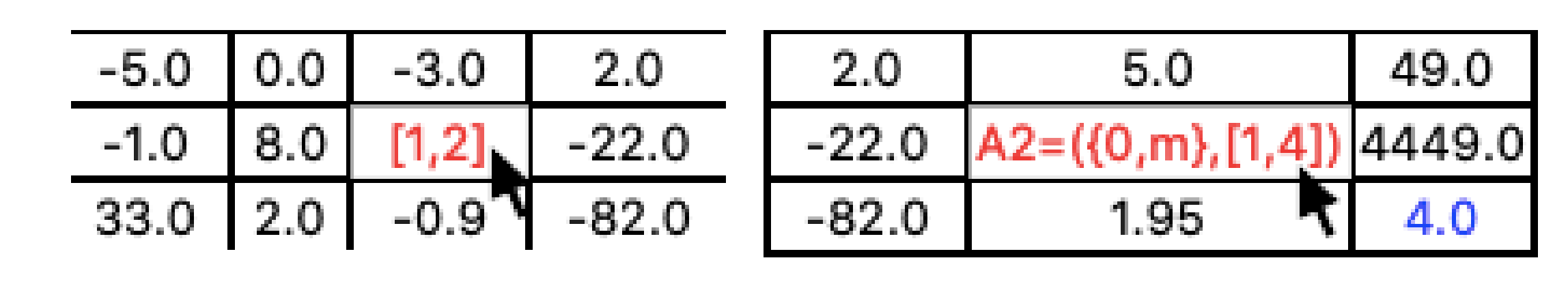
The agents are represented by the blue color of the text. By moving the mouse cursor to the position of the agent, the user obtains detailed information about it in the following form: $A_i=(obj1,obj2,[PosX,PosY])$, where i is the index of the agent, $obj1$ and $obj2$ are the objects inside this agent, and $PosX$ and $PosY$ are the coordinates of its position. This behavior of the application can be seen in Figure 12.

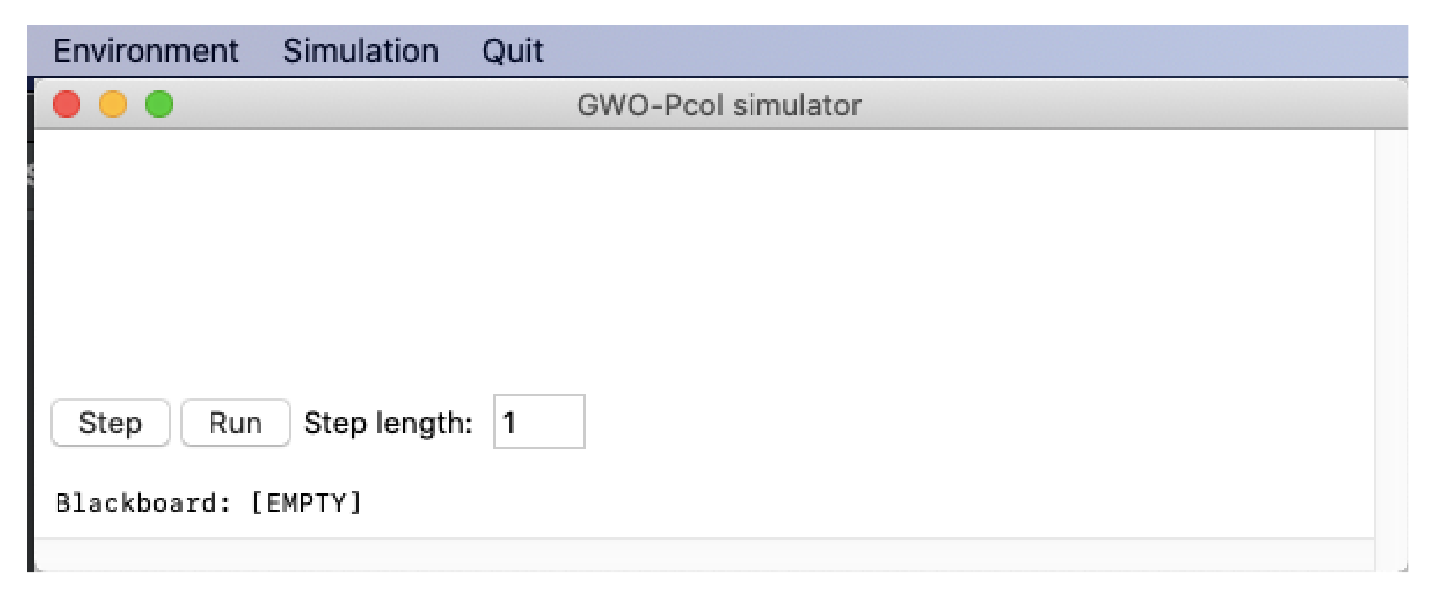
8.3. Buttons Controlling the Simulation

The Step button runs the predefined number of steps of the simulation. The number of steps is defined in the field Step length. The iteration is a set of these steps. New iteration starts when each agent performed all of the steps that are needed before the synchronization.

The Run button runs the simulation, until the simulation terminates reaching the termination criterion, or the iteration reaches the maximal value, or when none of the delta agents can move. Figure 13 displays the buttons controlling the simulation.

8.4. Text Field for the Backboard

The text field for the blackboard is set as read-only and it has two lines. Each line displays the vectors of the blackboard.

This text field is initialized together with the agents and updated at the end of each iteration, as it was described in section Blackboard. Figure 6 presents the visualization of the blackboard in the application.

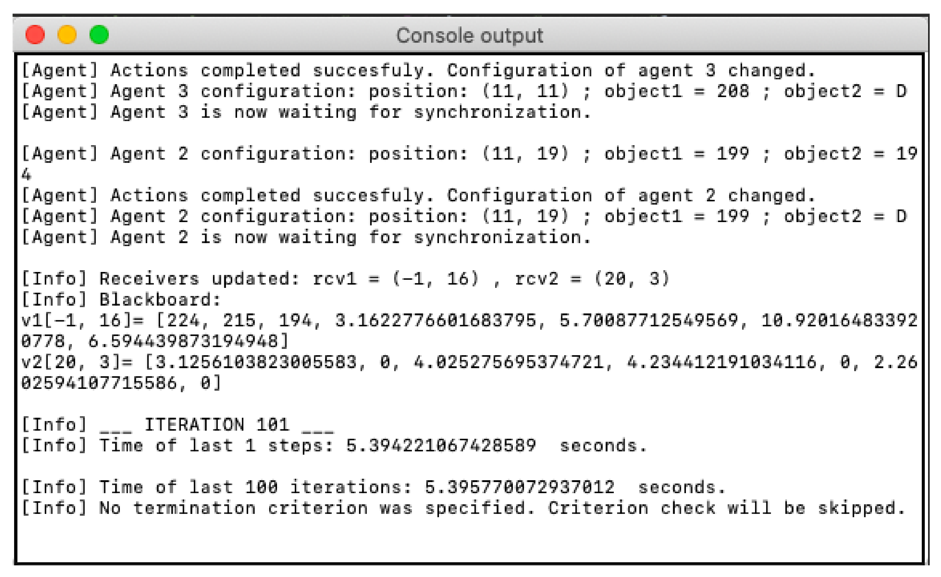
8.5. Console Output

By default, the application sends the console text to the default printer (typically, command line in Windows, Bash, or Shell console in Unix based OS).

While the application can only be used in the graphic interface, the console output can be redirected to a new text field window (see Figure 14). This functionality can be enabled in the application menu (Menu → Simulation → Console output) and it is equivalent to the default console form.

In the console, the user can monitor text messages with the following information in real-time:

• the information about the state of the agents (see Table 5), and
• application error messages (see Table A1 and Table A2).

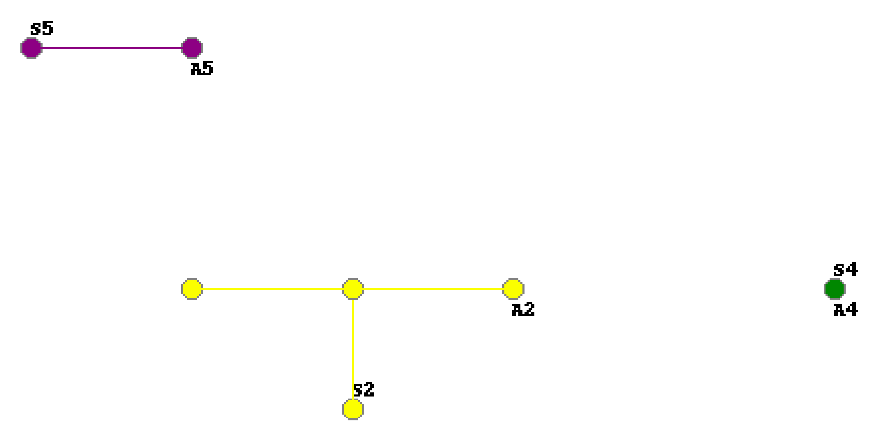
8.6. Canvas Drawing the Simulation

The function Canvas drawing the simulation is used by the user for an overview of the area of the environment that is searched by the agents. An example can be seen in Figure 15. The environment points are scaled into an $800\times 600$ canvas area (the size of the environment is adapted to the size of the canvas). The points that have already been visited by the agents are circled by different colors. Each color corresponds to the particular agent. If two different agents visit the same position, the color of the agent that last visited it is used. In the canvas, the initial position of the agent is described by text $S_i$, and the current position is described by $A_i$, where i is the index of the agent. The visited points are connected by an edge (line) of the same color as the color of the agent, according to the movements of the agent in the environment.

In the future, we plan to implement an option for showing the full path of each agent separately. This improves the clarity of the output of this functionality, and the user will be able to identify the positions visited by a particular agent.

9. Example of Use

Let us give the example of the use of the application. This example can also serve as the application guide.

As the first step, the user checks or modifies the rules in the file “$rules.xls$”, according to Section 5.2. Subsequently, the user launches the application using the executable file in the application directory structure. The main application window will open.

Figure 16 shows the main application window at startup. At this point, the canvas displaying the simulation is empty, so the environment should be loaded (Menu → Environment → Load environment). A file dialog window (see Figure 8) opens, and the user selects an environment file ($.env$ file).

If the application is not run from the command line or console, then it is useful to open the console output in a separate window at this point (Menu → Simulation → Console output). If the application is run from the command line or console, the text output is directly available in the command line or console. It is useful (and sometimes necessary) to monitor the current configuration of the simulation and individual agents.

When the environment file has been selected and displayed on the canvas, the simulation can be initialized (Menu → Simulation → Initialization). Before initializing the agents and placing them into the environment, it is possible to adjust the configuration of the algorithm, and the positions of the agents, in separate windows (see Section 5.3, and Table 4).

The user controls the application using the buttons that are described in Section 8.3. During the simulation, the user can monitor the console output, the canvas visualizing the simulation (to see agents and their movements in the environment), and the blackboard (for example, to see the best values of Alpha, Beta, and Delta agents).

If the optimal value has been found (termination criterion reached) or the simulation is stagnant, i.e., increasing the iterations no longer improves the results, agents no longer move, there is no reason to continue the simulation. At this point, the user can use canvas drawing the simulation (Menu → Simulation → Draw simulation) to determine which area of the environment was searched (scanned).

The application can be terminated at any time (Menu → Quit → Quit application).

10. Testing

The first version of the simulator was not acting as desired, but the complications were expected. In the first derivation steps, most of the wolves tried to be the Alpha wolf, and they tried to write to the alpha position on the blackboard. This behavior of the simulator led to the situation when the Omega wolves were without the lead and they reached the final configuration soon, and the simulation stopped unsuccessfully very often, giving no result. When considering these results, we decided to make a slight change in the behavior of the wolves in the first steps of the derivation. Once the wolf tries to write to the alpha position (on the blackboard) unsuccessfully, it is allowed to try to write to the beta and delta position, respectively. This modification is still in the scope of the P colonies, and we were not forced to introduce some outer mechanism setting the hierarchy of the pack. The wolves were able to set the hierarchy themselves, and the simulation proceeded as expected.

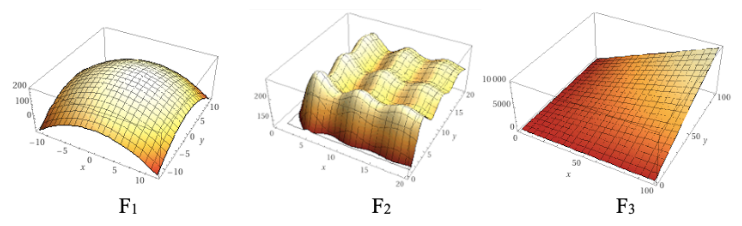
Let us focus on the performed testing of this implementation. While the application is the simulator of the 2D P colony, it is a bit problematic to compare the time the 2D P colony and GWO consume; therefore, we will measure and compare the performance of the algorithms in the iterations.

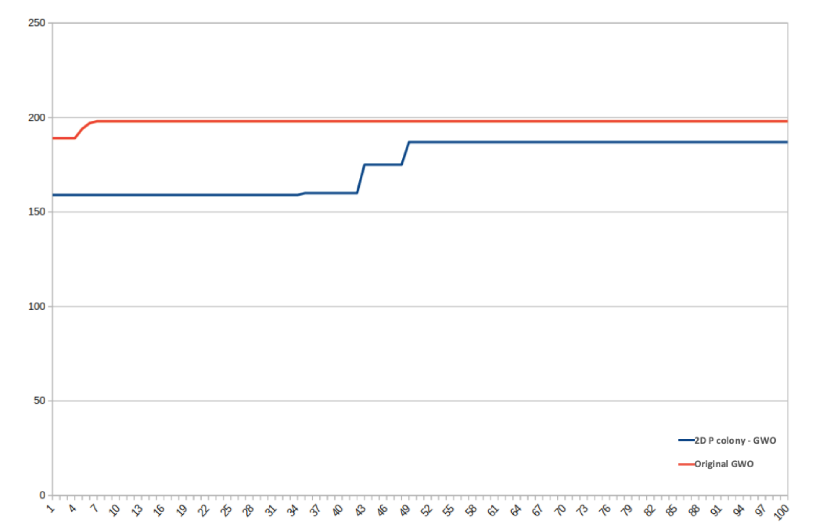
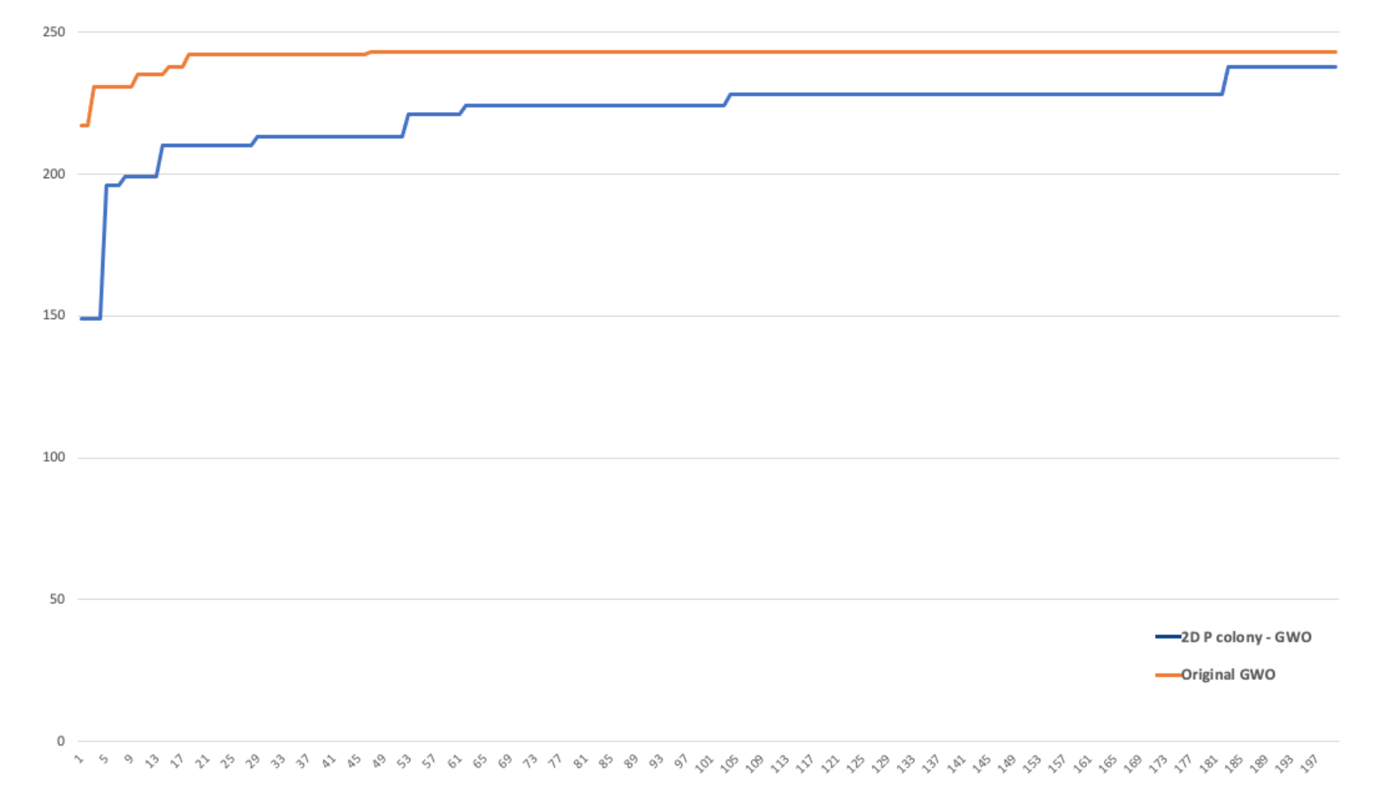
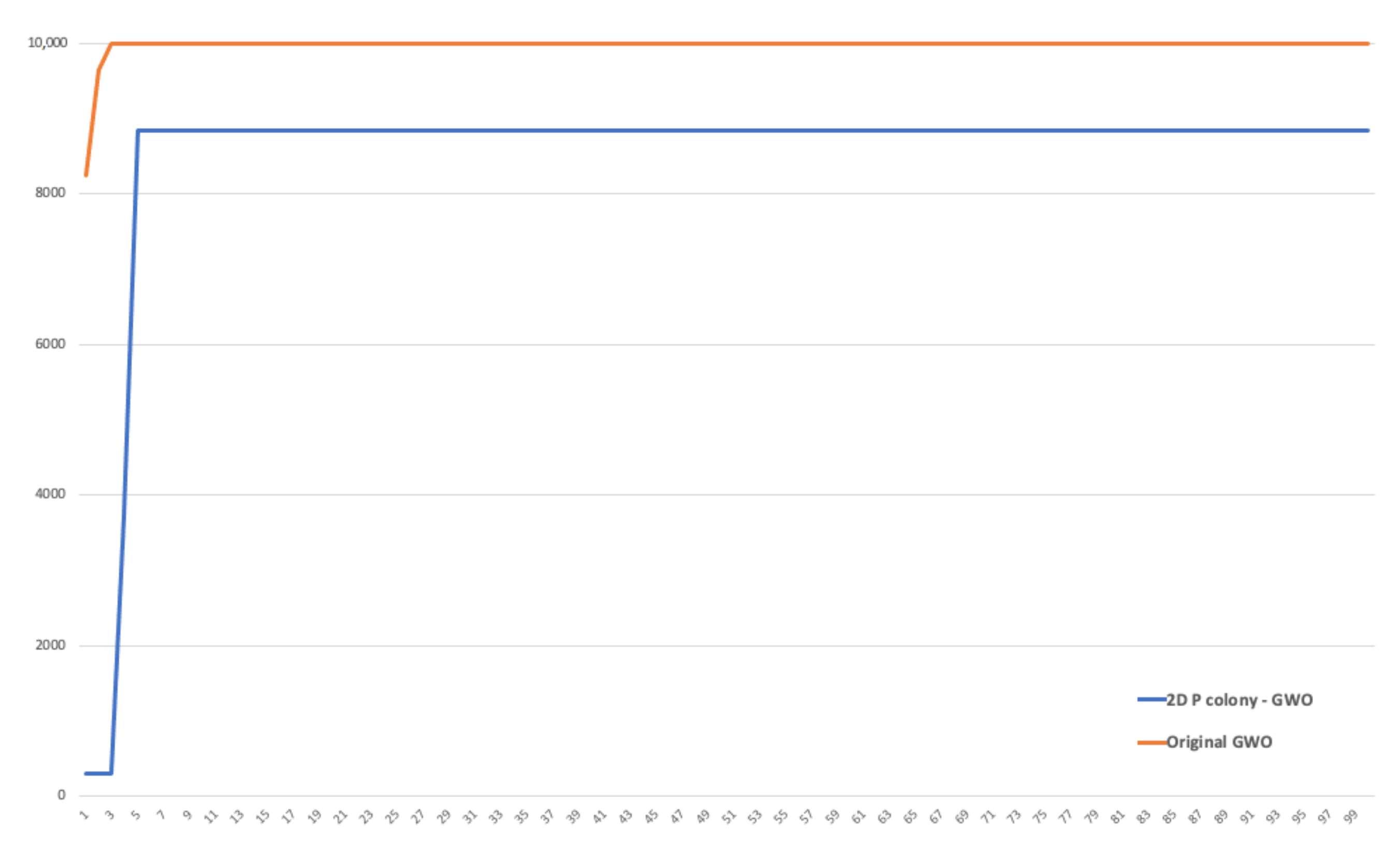
We compared the performance of the original GWO algorithm and our 2D P colony simulator. The number of agents (wolves) was set to 6 in both of the algorithms (typical number of wolves in packs). The fitness functions used for optimization can be seen in

Table 6. The functions used for testing the performance.

Fitness Function	Optimization Goal	Maximum Number of Iterations
$F_1=-\left(x^2+y^2\right);x,y\in \left(-10,10\right)$	Find maximum	100
$F_2=-100\left(\frac{sin\left(x\right)}{x}+\frac{sin\left(y\right)}{y}\right)+200;x,y\in \left(1,20\right)$	Find maximum	200
$F_3=x\ast y;x,y\in \left(0,100\right)$	Find maximum	100

and the 3D plots can be seen in Figure 17.

The test results are summarized in the

Table 7. Summary of testing.

Comparison	Original GWO			2D P colony – GWO
Function	F${}_1$	F${}_2$	F${}_3$	F${}_1$	F${}_2$	F${}_3$
Number of agents	6			6
The real global extreme of function	200	243	10,000	200	238 (discretized)	10,000
Best fitness value in the initialization phase	189	217	8236	159	149	304
Convergence after iterations	6	47	3	49	182	5
Best solution found	198	243	10,000	187	238	8836

, and the charts are in the pictures Figure A1, Figure A2 and Figure A3.

The original GWO algorithm found the optimal value faster and more accurately in all three cases, when compared to the implemented model. The implemented model is slower, especially because of the size of the step of the agent. It is at most one in one iteration, i.e., the 2D P colony agent can in one step move only one position further (move left, right, up, or down), unlike the GWO, where the movement of the agent is not that limited. This is also one of the reasons the 2D P colony does not achieve the results of the same quality.

Another factor influencing the 2D P colony performance is the position of the agent. Once the agent gets to the position in which there is no better position in the near vicinity, i.e., the agent is stuck in some local extremum, it will not change its position and is not able to find the optimal value anymore. This problem of larger areas in an environment, with the same fitness value of several adjacent points, can be eliminated by a better discretization of the fitness function.

Despite the results of the tests, the proposed model and its implementation can be considered to be a success. Firstly, we have proved that such a simple theoretical model, like the 2D P colony, is able to successfully solve the optimization problem. The model and/or the rules can be adjusted based on these results, so we will be able to reach better performance.

11. Conclusions

In previous research, we proposed a model of 2D P colony simulating the behavior of the pack of wolves in the same manner as in the Grey wolf optimization algorithm. In [13,14,15], we introduced a numerical version of the 2D P colony that is equipped by the blackboard, where the environment is represented by the discrete values of the fitness function. In this paper, we introduced the computer simulator of the extended version of the 2D P colony, and present the results of the simulations.

We present the complete description of the algorithm, from the basic analysis up to the description of the algorithm, including its inputs. We have shown the design of the model, including the methods and tools used in the implementation. This results in the application that provides the user the console output for a full overview of information regarding the current configuration of the system during the simulation, and the graphical interface used for the visualization of the simulation. In Section 9, we describe the use of the application. This section can be sensed as the application guide.

The tests we made resulted in the modification of the model that was proposed in [13,14,15]. Further tests of our application and comparison to the GWO are presented in Section 10. In this section, we also discuss and explain the results. Our model, which is composed of very simple agents, successfully simulates the GWO, and it can solve the optimization problems.

The implementation allowed us to study and improve the behavior of our model. For further research, we plan to optimize the model and the application in order to obtain a smoother simulation and hopefully better results.