Modelling Cell Metabolism: A Review on Constraint-Based Steady-State and Kinetic Approaches

Abstract

Studying cell metabolism serves a plethora of objectives such as the enhancement of bioprocess performance, and advancement in the understanding of cell biology, of drug target discovery, and in metabolic therapy. Remarkable successes in these fields emerged from heuristics approaches, for instance, with the introduction of effective strategies for genetic modifications, drug developments and optimization of bioprocess management. However, heuristics approaches have showed significant shortcomings, such as to describe regulation of metabolic pathways and to extrapolate experimental conditions. In the specific case of bioprocess management, such shortcomings limit their capacity to increase product quality, while maintaining desirable productivity and reproducibility levels. For instance, since heuristics approaches are not capable of prediction of the cellular functions under varying experimental conditions, they may lead to sub-optimal processes. Also, such approaches used for bioprocess control often fail in regulating a process under unexpected variations of external conditions. Therefore, methodologies inspired by the systematic mathematical formulation of cell metabolism have been used to address such drawbacks and achieve robust reproducible results. Mathematical modelling approaches are effective for both the characterization of the cell physiology, and the estimation of metabolic pathways utilization, thus allowing to characterize a cell population metabolic behavior. In this article, we present a review on methodology used and promising mathematical modelling approaches, focusing primarily to investigate metabolic events and regulation. Proceeding from a topological representation of the metabolic networks, we first present the metabolic modelling approaches that investigate cell metabolism at steady state, complying to the constraints imposed by mass conservation law and thermodynamics of reactions reversibility. Constraint-based models (CBMs) are reviewed highlighting the set of assumed optimality functions for reaction pathways. We explore models simulating cell growth dynamics, by expanding flux balance models developed at steady state. Then, discussing a change of metabolic modelling paradigm, we describe dynamic kinetic models that are based on the mathematical representation of the mechanistic description of nonlinear enzyme activities. In such approaches metabolic pathway regulations are considered explicitly as a function of the activity of other components of metabolic networks and possibly far from the metabolic steady state. We have also assessed the significance of metabolic model parameterization in kinetic models, summarizing a standard parameter estimation procedure frequently employed in kinetic metabolic modelling literature. Finally, some optimization practices used for the parameter estimation are reviewed.

1. Introduction

Expanding the modelling paradigm, from a microscopic description to systems biology perspective, has offered a deeper capacity to describe cell behaviour and its interaction with extracellular environment. The improvement was necessary to address complex problems related to the characterization of intracellular events [1,2,3]. Indeed, one-reaction models have then rapidly evolved to reaction network-level models, and recently reached a genome-wide level when applicable. Various mathematical approaches have been proposed to first integrate a reaction network and stoichiometry, for then integrating reaction kinetics and regulation mechanisms. While evolving, models have gained the capacity to question cell behaviour by both interpolating within and extrapolating from experimental data, for then allow extracting data that are tedious to impossible to be directly acquired, such as intracellular metabolic flux rates [4]. The predictive power that network-level models offer is an important advantage of such systemic mathematical representation compared to heuristics approaches. In fact, metabolic models have evolved to encompass higher levels of the knowledge regarding a biosystem, i.e., from gene to protein to reaction, to thus enhance the predictive power. Cell metabolism is a complex biosystem of study, even for unicellular organisms. Indeed, metabolic modelling is particularly challenging because many cellular functions are the result of a combination of factors. Therefore, unravelling causal relations and correlations between an observed phenomenon and its associated factors necessitates a model capable of describing the underlying biosystem, the network of biochemical interactions, and their connectivity and regulation. A model is still a modest approximation [5]. The merits and drawbacks of a model are determined by adequacy to describe a biological reality, further, a compromise between model correctness and the extent to which it is mathematically tractable is unavoidable [6]. Thus, simplifying assumptions must be considered making a metabolic model definite in its scope and solvable regarding available experimental data. These assumptions are a consolidation of heuristics experiences for a model, the current knowledge of the biosystem and of its interaction with its surroundings. Typical assumptions concern the cell compartments homogeneity level, a diversity in biological time scales, the level of distributing versus lumping entities of interest, among others. These assumptions are particularly of interest because they are the main factors determining the relation between an observation in reality and the result of the simulation of an abstract mathematical model. The required metabolic modelling approach is shaped to accommodate the assumptions and provide the sought-after applications [3,7,8,9]. The metabolic network models have been developed to understand the dominant qualitative features of cell metabolic behaviour in a bioprocess [10], or in a metabolic disease [11]. A comprehensive metabolic model can also improve conventional wisdom regarding the cell metabolism by making important corrections, such as gap-filling reactions suggested by genome-wide metabolic models [12,13]. When required to interfere with cell functioning, a metabolic model can contribute to discovering new strategies [11,14,15], and to organize the disparate accumulated information into a coherent body of practical knowledge [3,16]. In a complex system such as the metabolic network of the cell, a model helps to think (and calculate) logically about what components and interactions are important and what other components can be neglected [17]. However, the extent of progress in the model application to accomplish each of these goals depends on several factors, including the industrial importance and the scientific significance of sought-after results. Based on this premise, metabolic modelling has gained substantial importance to enhance bioprocess optimization [18,19], where the increased efficiency leads to cost reduction in million-dollar order of magnitude, and to develop metabolic therapies [11,14], i.e., to push forward cancer treatment. In a broad classification, metabolic models are divided into four categories based on the capability of the model to distinguish between sub-populations of biomass (unsegregated/segregated) and the extent of recognizing the intracellular biochemical components (unstructured/structured) [17,20], (Figure 1).

In this review, we have clustered modelling approaches which are mostly understood as unsegregated and structured. Thus, such a mathematical model describes multi-compartment average cell and when it is desired the model extends the description to the whole population by taking into account the quantity (size) of the population, i.e., biomass concentration. Present approaches proposed in literature were compared based on their ability to elucidate the structure of a network, to then characterize allowable and empirical flux distribution, and to finally take into account flux dynamics regulation. This review is not by any means a comprehensive tabulation of the exhaustively diverse range of the published metabolic models, but a methodology motivated review of the keystones of metabolic modelling. Thus, significant trade-offs between any two categories were acknowledged. Also, from another crucial perspective, the capability of the models under steady state and dynamic state of the metabolic network is assessed. The revised modelling approaches have been used for severely different scales of metabolic systems and typically to serve distinct strategies, therefore, it deems essential to notice the context where models are primarily used to avoid confusion. When possible, a simple running example is used to illustrate the approach being discussed. The running example is first introduced in Figure 2.

2. Topological Representation of Metabolic Networks

2.1. Representation Based on the Graph-Theory

In this approach, cell metabolic networks are denominated Bio-Chemical Reactions Network (bio-CRN), including the reactions that govern the cell metabolism. Owing to genome sequencing technologies, annotated genomes for several organisms made possible to reconstruct metabolic network accounting for the major active constituents of the cell, i.e., proteins, DNA, RNA and other metabolites [21,22]. Modelling approaches based on the graph theory have been used to unravel network complexity by quantitative methods. In (the major variants of) this approach, the metabolic network substrates are modelled as nodes of the graph and reactions as the (directed) edges [21,23]. It has been shown, in comparative studies for different species that the graph of a metabolic network can be modelled by a scale-free connectivity structure [24]. In a scale-free structure, the probability distribution of finding a node with k connections follows a power-law function, i.e., $P\left(k\right)\approx k^{-\lambda }$, with $\lambda$ being a species-specific positive constant. In a metabolic network context, it means that the probability of finding a substrate involved in k reactions decreases with a power-law relationship to the increasing number of reactions [23,25,26]. (refer to Figure 1 of [21] for illustration of the connectivity structures.)

Reconstruction of the metabolic network for 80 fully sequenced organisms taken from eukaryotes, archaea and bacteria conclude that most of the metabolites participate in a few reactions and a few ones drive many reactions, with these latter defined as hub-metabolites [21,24,26,27]. Interestingly, this statistically heterogeneous distribution of metabolites connectivity resembles an error-tolerant system structure, which is found in human-made networks such as the Internet [28]. It was shown that random elimination of reactions due to mutations of enzyme-coding genes are tolerated by metabolic networks and the structural redundancy allows the modified metabolic networks to result in viable reorganizations of the metabolic routes, i.e., the in-silico model maintained the potential to support growth [29]. In fact, it is argued that “the small world architecture” of metabolic networks, which refers to the scale-free structure, “may serve to minimize transition times between metabolic states…” [26] as well. On the other hand, network behaviour, i.e., fluxes rates and distribution, is sensitive to changes of so-called hub-metabolites [24,30,31], which motivated further structural investigation of these special nodes. A sub-network mostly made of hub-metabolites is named the giant strong component of a metabolic network, and it represents the core metabolites typically consisting of less than one third of the total metabolites included in the metabolic network [24]. In [26], the authors identify a node in the substrate graph as a hub-metabolite if its degree exceeds the mean metabolite degree of the network by three times the standard deviation. Moreover, considering the most linked metabolite is ranked first in a network, and it is a shared metabolite between tens of organisms with an average rank of R, it has been shown that metabolites in higher average ranks see less deviation in their ranks among the different organisms. Conversely, the metabolites of lower average ranks, i.e., the ones participating in a few reactions, show species-specific changes in the number of reactions they are participating in.

Topological analysis of metabolic networks structure also provides the average reaction path between any two substrates. As expected, this number increases with the addition of more metabolites to the network. However, some individual metabolites then become more and more connected, thus the average length of reaction paths remains in a much narrower range compared to the range of added metabolites. As an example, if the number of metabolites integrated in the metabolic network increases from 200 to 1000, the average reaction path increases from 4 to 12 (refer to Figure 5 in [23]). Worth mentioning, the calculated average reaction path increases when the connections through the energetic metabolites, such as $ATP/ADP$, $NADH/NA{D}^{+}$ and $NADPH/NAD{P}^{+}$, are eliminated, highlighting their significant role as co-metabolites of many reactions. Excluding these metabolites, the ten most connected metabolites are the intermediates in the glycolysis pathway (Glycerate-3-phosphate, D-Fructose 6-phosphate, D-glyceraldehyde-3-phosphate), the intermediates in the pentose-phosphate pathway (D-ribose-5-phosphate, D-xylulose-5-phosphate), pyruvate and acetyl-CoA, the precursor for purine and histidine synthesis (5-phospho-d-ribose 1-diphosphate), L-glutamate and L-aspartate [23].

2.2. Representation Based on the Petri net Theory

Petri net theory supports another topological oriented modelling approach of metabolic networks [32,33,34]. A Petri net is a directed graph, whose nodes have two different types, namely, places and transitions. Thus, substrates (and products) are considered as the places, and reactions are the transitions. In this approach, one end of an edge is connected to a metabolite and the other end is connected to a reaction. Therefore, as opposed to the graphs reviewed in Section 2.1, in Petri net graphs edges are not representative of reactions. Instead, edges have weights resembling the stoichiometric coefficients [35]. Petri net models provide a reliable analysis of the consumption/production relations but not of regulatory interactions. However, several extensions of the primary formalism have been introduced to increase the quantitative suitability of Petri net theory for biological systems analysis. For example, coloured Petri nets, stochastic Petri nets [36,37], self-modified Petri nets [38,39], and hybrid functional Petri nets [33]. Nevertheless, the Petri net representation of metabolic networks still deserves more methodological developments.

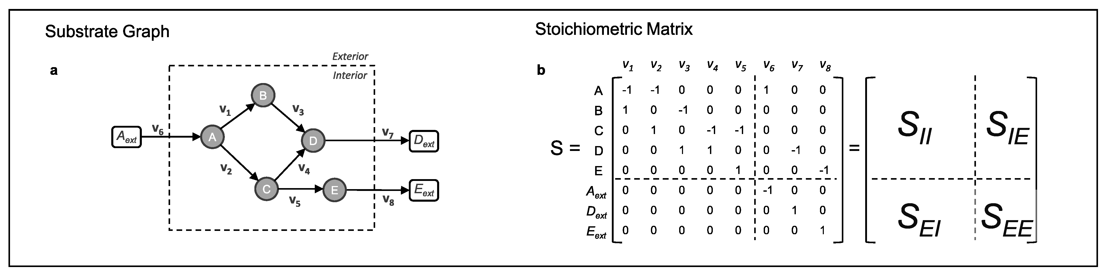
2.3. The Stoichiometric Matrix of a Metabolic Network

As for a chemical reaction, the stoichiometry of a biochemical reaction tells the relative number of moles on either side of a reaction involving an enzyme in a balanced reaction [3]. In a bio-CRN, the matrix of stacked stoichiometric vectors of all the network reactions forms the stoichiometric matrix of the reaction network. The stoichiometric models of metabolic networks for prokaryotic and eukaryotic cells are available in literature [40]. The stoichiometric matrix for a metabolic network with m metabolites and n reactions is as follows:

$$S_{m\times n}={\left(\begin{array}{c}{s}_{i,j}\end{array}\right)}_{m\times n}\{i=1,\dots ,m|j=1,\dots ,n\}$$

(1)

where the i th row consists of reaction coefficients for metabolite i, with regard to (w.r.t) all reactions of the network, $s_{ij}$ is the coefficient of metabolite i in reaction j. A negative $s_{ij}$ implies that the metabolite i is on the left side of a reaction j and thus assumed to be consumed, if positive it is receiving flux of matter in the reaction j ($v_j$), and zero if it does not participate in the reaction j:

$$\begin{array}{cc}\hfill {\displaystyle \frac{d{x}_i}{dt}}& =\sum _{j=1}^n{s}_{ij}^{+}{v}_j-\sum _{j=1}^n{s}_{ij}^{-}{v}_j,i=1,\cdots ,m\hfill \end{array}$$

(2)

Therefore, we have one column vector for each reaction and Equation (2) can be written in matrix-vector notation for the whole metabolic network as follows:

$$\begin{array}{cc}\hfill {\displaystyle \frac{d\overrightarrow{x}}{dt}}& =S_{m\times n}\overrightarrow{v}\hfill \end{array}$$

(3)

The stoichiometric matrix can be reshaped into four partitions, each of which with specific characteristics (Figure 2).

Structural analysis of metabolic networks can be more elegantly performed by using the matrix formalism instead of topological theories, as it is transferable to a graph representation while such transfer from the topological representations is not always possible [3,6]. Either way, the analysis is not restricted only to genome-scale metabolic networks, and it can be efficiently used in an early step of modelling to draw a non-intuitive sense of network reactions connectivity. However, relying solely on structural information to extract connectivity interactions suffers from the flawed assumption that every biochemical reaction is worthing same weight, regardless of its level of activity. Therefore, the structural analysis results can hardly be directly useful for investigating the cellular mechanisms for flux regulation [41,42]. Contribution of the stoichiometric matrix to the formulation of the further approaches is fundamental. The algebraic properties of stoichiometric matrix and nowadays matrix computation capacity has fuelled further use of the stoichiometric matrix as an important part of any metabolic mathematical models. The significance of its role in the representation of metabolic networks will become evident through the following sections.

3. Metabolism Is a Constrained System

Approaches based on the metabolic steady state hypothesis have been first proposed for estimating theoretically active enzymatic reactions [43,44,45,46], and to estimate metabolic flux rates from the reaction network stoichiometry and experimental time-data of extracellular metabolite concentrations [11,47,48,49,50,51,52]. The mass conservation constraint at the steady state is formulated through the stoichiometric matrix for a network of biochemical reactions at any size, and this constraint has a central role in the determination of the solution space in many approaches (following sections) [53]. The observation that the changes of intracellular fluxes occur at a faster dynamic compared to the changes of the extracellular concentrations supports the validity of the steady state assumption [54,55]. A detailed mathematical justification of the (pseudo) steady state assumption in the mathematical modelling of biochemical reaction networks is proposed in 1983 in [54], however, in the context of this review article, this assumption is valid at constant exponential growth phase in batch cultures, and in continuous cultures operating at steady state [56]. The advantage of the constraint-based modelling is that these approaches do not need to deal with enzyme kinetics and post-translational regulatory mechanisms [57]. In the following, we review the most relevant approaches and the associated constraints that are imposed on metabolic networks.

3.1. The Null Space of Stoichiometric Matrix

From a mathematical point of view, the stoichiometric matrix S, denotes a linear mapping of the reaction rate vector into the space of accumulated concentration time derivatives of metabolites [58]. To illustrate, consider N to be a linear mapping function, let:

$$N:{\mathbb{R}}^n\to {\mathbb{R}}^m$$

be defined by:

$$N\left(\left[v_1,v_2,\cdots ,v_n\right]\right)=\left[{\dot{x}}_1,{\dot{x}}_2,\cdots ,{\dot{x}}_m\right]$$

(4)

since N is linear, we can write:

$$\begin{array}{cc}\hfill N\left({\overrightarrow{v}}_{(n\times 1)}\right)=& v_{1}N\left({\overrightarrow{e}}_1\right)+v_{2}N\left({\overrightarrow{e}}_2\right)+\cdots +v_{n}N\left({\overrightarrow{e}}_n\right)\hfill \end{array}$$

(5)

$$\begin{array}{cc}\hfill =& {\left[N\left({\overrightarrow{e}}_1\right)N\left({\overrightarrow{e}}_2\right)\cdots N\left({\overrightarrow{e}}_n\right)\right]}_{(m\times n)}{\overrightarrow{v}}_{(n\times 1)}\hfill \end{array}$$

(6)

$$\begin{array}{cc}\hfill =& S_{(m\times n)}{\overrightarrow{v}}_{(n\times 1)}={\overrightarrow{\dot{x}}}_{(m\times 1)}\hfill \end{array}$$

(7)

For the particular case of metabolic network operating at steady state, we have $S_{(m\times n)}{\overrightarrow{v}}_{(n\times 1)}^{*}={\overrightarrow{\dot{x}}}_{(m\times 1)}=\overrightarrow{0}$. The set of vectors ${\overrightarrow{v}}_{(n\times 1)}^{*}$ are linearly dependent to the members of the basis for the null space (Equation (8)) and thus, a subset of the null space of the stoichiometric matrix S (Equation (9)). Where r is the rank of stoichiometric matrix S, the basis for the null space is a set with $q=(n-r)$ linearly independent column vectors of dimension n, which generates the null space for stoichiometric matrix S when spanned [58].

$$\begin{array}{cc}\hfill & \mathcal{K}\left(S\right)=\{{\overrightarrow{b}}_i\in {\mathbb{R}}^n(i=1,\cdots ,q)|S.{\overrightarrow{b}}_i=\overrightarrow{0}\mathrm{and}{\overrightarrow{b}}_i.{\overrightarrow{b}}_j=\overrightarrow{0}(i\ne j)\}\hfill \end{array}$$

(8)

$$\begin{array}{cc}\hfill & \mathit{Null}\mathit{space}\left(S\right)=\mathit{span}\{{\overrightarrow{b}}_1,\cdots ,{\overrightarrow{b}}_q\},q=(n-r)\hfill \end{array}$$

(9)

where $\mathcal{K}\left(S\right)$ denotes the basis for the null space of stoichiometric matrix S.

3.2. Metabolic Pathway Analysis (MPA)

Metabolic networks are an interconnected set of the metabolic pathways which interconnect at branch points and through shared metabolites. It is common, inside a metabolic network, to have several redundant routes for the transformation of one given metabolite to another. It is particularly true for linking external substrates to external metabolic products [59,60]. These multiple routes, which obey to mass conservation principle at steady state, are considered a main cause of biological robustness [61,62]. Thus, model development by the decomposition and characterization of a metabolic network into definitive pathways has attracted attention to allow identifying the dominant routes [9,63,64]. Particularly, MPA modelling approaches adapt a convex basis analysis methodology to estimate a theoretically feasible relative flux distribution. In MPA, component pathways of the network and genetically independent reaction pathways are identified [9,65,66], such insight is particularly of interest in gene-knockout and synthetic pathway construction studies [67], and in designing stoichiometrically growth-coupled overproduction in production host organisms [68].

MPA is usually used as an umbrella term for the approaches based on the notion of elementary flux mode analysis (EFMA). A flux mode is a flux distribution vector that satisfies the mass conservation constraint for the intermediate metabolites at steady state, and does not violate direction restriction of irreversible reactions. The term flux modes was coined by Schuster et al. [6,63] in 1994, to address the independent enzyme sets responsible for a component pathway. If it is not possible to further decompose a flux mode to a linear combination of simpler flux modes, it is considered as an elementary flux mode (EFM). In biochemical terms, it is a minimal set of enzymes “that can operate at steady state, with all irreversible reactions used in the appropriate direction” [65]. In mathematical definition, the convex basis vectors for the null space of the stoichiometric matrix of a metabolic network represent EFMs [69] (see Figure 3 and Table S1, Supplementary Materials, for properties of the different MPA methods). The algebraic tools and methodologies of MPA have been continuously enhanced to address shortcomings of the EFMA and therefore enabling EFM-based methods to claim more applicability in systems metabolic engineering. EFMs reproduce all the admissible reaction pathways at steady state in an unbiased manner, therefore, enumerated EFMs of a large metabolic model can quickly exceed computational capacity of a typical computing system of the date. However, various studies show that usually a small percentage of these calculated EFMs are biologically and thermodynamically feasible [70,71], or relevant to the metabolic scenarios under study [72]. Thus, the integration of constraints from biology and thermodynamics, in addition to the introduction of more efficient computational algorithms are utilized to ameliorate the computational cost of enumerating EFMs for genome-scale models.

Extreme pathway analysis (EPA) is one closely related method to EFMA, in its formulation, an important condition is the net direction of each reaction. Therefore, the reactions that can be reversible may flow in two different directions at different states of cell metabolism. Knowing that, EPA is assumed to extract the minimal subset of EFMs [73]. Considering the n-dimensional vector of intracellular fluxes, EFMs form a convex cone in the solution space, while extreme pathways characterize the edges of this polyhedral cone [53,71,74]. Even though EPA is computationally less demanding than EFMA [75,76], it may exclude possibly important reaction routes and thus causes loss of valuable structural information [77]. Another important mathematical framework used for MPA is Minimal Cut Set (MCS) approach, which was introduced in 2003 [78]. A MCS with respect to an objective reaction represents a set of other reactions of metabolic network, whose inactivation will make it impossible for the objective reaction to appear in any steady state flux distribution of the network. However, since implementation of MCS can simultaneously eliminate a desired function of metabolism, constrained minimal cut sets (cMCS) was introduced to circumvent this limitation by allowing for the definition of a set of desired flux modes to be preserved during the enumeration process [79]. Recently, Axel von Kamp and Steffen Klamt enhanced the computational algorithms of MCS enabling this method to operate on genome-scale level, in a comprehensive computational investigation of growth-coupled production, the authors show capability of the approach to investigate feasibility of coupling different metabolites to growth in five major bioproduction host organisms [68]. Use of these approaches complemented promising methods to identify co-regulated reactions and co-expressed genes [80], and composition of the minimal required substrates in order to produce valuable metabolic products [80,81] (see Table 2.1 in [82] for a list of software packages for enumerating EFMs). Authors in [83] generated hypotheses for strain metabolic engineering guided by the MCS computation of the metabolic network of an industrial microbe (Pseudomonas putida). The experimental implementation of the guided predictions enhances titer, rate and yield of the microbe by coupling its growth to bioproduction, i.e., production starts from late exponential phase.

3.3. Metabolic Flux Analysis (MFA): Admissible Metabolic Fluxes

Flux quantification in a metabolic system reveals significant information about the cell physiological state. Such information, particularly characterizes the cell response to genetic manipulation or changes in its environment, thus, may be used to improve a bioprocess toward predefined optimization objectives [17,84]. Moreover, it was shown in several studies that the rates of exchange reactions, i.e., intermembrane transport reactions, can be used not only to quantify the rates of the intracellular reactions, but also to describe global processes taking place in the corresponding metabolic state of the cell [17,84,85,86]. In a comprehensive metabolic network, the number of metabolites is typically smaller than the number of intracellular and exchange reactions combined. Thus, the associated stoichiometric matrix renders an under-determined system of equations, where the metabolites form balance equations, and the reaction rates are unknowns. When the system of equations is solved, MFA provides an empirical flux map [87,88,89], instead of the relative distribution of the fluxes provided by MPA. The mathematical formulation is as follows [55]:

$$\begin{array}{cc}\hfill S.\overrightarrow{v}& =0\hfill \\ \hfill \left[\begin{array}{cc}{S}_u& S_k\end{array}\right]\left[\begin{array}{c}{\overrightarrow{v}}_u\\ {\overrightarrow{v}}_k\end{array}\right]& =0\hfill \\ \hfill {\overrightarrow{v}}_u& =-\left[{\left(S_u^T{S}_u\right)}^{-1}{S}_u^T\right]S_k{\overrightarrow{v}}_k\hfill \end{array}$$

(10)

where the vector $v_u$ represents unknown fluxes, the vector $v_k$ the measured (known) fluxes, and $S_u$, $S_k$ the stoichiometric matrix subsets for unknown and measured fluxes, respectively.

To have a determined system, the degree of freedom of a system must equal zero. Generally, some reaction pathways are excluded from a comprehensive metabolic network to qualify it for MFA [90], and experimental data regarding concentration of medium components are used to further decrease the degree of freedom, i.e., identifying more exchange reactions. Measurements provide the estimation of cell concentration and uptake/secretion rates, which are the characteristic parameters of cell activity. Conversely, the degree of freedom increases as a result of the branches of pathways diverging and then rejoining later in the network, reversible reactions and metabolic cycles. These structures add reaction columns to the stoichiometric matrix, which are linearly dependent to the existing ones [91,92]. For instance, the authors in [93] show that in a mammalian cell, it is essential to determine the uptake/secretion rates of ammonium and the secretion rate of either CO₂ or O₂. Because these are the cometabolites of the TCA cycle reactions, thus, determination of them enhances the observability of the fluxes in the TCA cycle. However, generally the balance equations alone are not capable of addressing such issues, therefore, additional constraining balance equations must be introduced to determine the system and consequently solve for the unknown fluxes [91,92].

13C-Metabolic Flux Analysis

More sophisticated substrate labelling experiments can be performed to overcome limitations of MFA approach such as from reversible and cyclic reactions [85,86,94,95,96,97]. Metabolite and isotopomer balancing have been developed since 1995 [98]. In this method, a labelled substrate (e.g., 13C-glucose, 13C-glutamate, 14N-glutamine) is administered to the cell, leading to the labelled atoms in different metabolites and in the macromolecular biomass constituents and thus as well as in the secreted products [96,99]. Henry et al. [85,86], used 13C-MFA to optimize the timing of induction of a biphasic Chinese hamster ovary (CHO) cell culture, by assessing the intracellular flux maps before and after production induction. Parallel labelling experiments as an alternative to traditional single tracer experiments [100] was used by Antoniewicz et al. to characterize flux distribution in growth and non-growth phases of CHO cell culture [52], among numerous other applications of this method [84].

Chromatography methods are used to separate labelled and non-labelled metabolites from each other (i.e., metabolite identification), then, mass spectrometry is used to measure their abundance by mass determination (i.e., metabolite quantification). Thus, use of a coupled either liquid or gas-chromatography mass spectrometry apparatus (LC-MS or GC-MS) is a prevalent strategy for metabolite profiling [94,101]. MS is particularly more popular in comparison with nuclear magnetic resonance (NMR) and liquid-chromatography mass-spectrometry (LC-MS), because of its good performance, extensive databases, relative cost of operation and the ease of maintenance [102,103], but exact quantification is more straightforward with LC-MS because of the use of known calibration curve with standards. The acquired data has to undergo correction and normalization to provide the measurements in a form that has biological information content. Kanani et al. [104], discussed the main sources of biases which arise in GC-MS and troubleshooted some of these biases, following the efforts to standardize this methodology as an integral part of the metabolomics data generation [105,106].

The non-experimental stage of metabolite labelling flux analysis consists of solving the isotopomer balance equations by computational algorithms. However, the capability of these algorithms to provide interpretation of experimental data and to support strategic experimental design is limited. In fact, increasing the power of frameworks to model isotope labelling system, with the least (or no) loss of information, is an active topic of research [99,102,107,108]. Recently modified versions of 13C-MFA were used to overcome the challenges of measuring metabolic fluxes in the distinct compartments of the eukaryotic cells (e.g., cytosol, mitochondrion). In a recent article, the authors provide an updated detailed protocol to perform 13C-MFA for the quantification of intracellular fluxes [102], and in a comprehensive review the latest developments in the MFA has been described [90].

4. Constraints Augmented with a Hypothesized Objective Function for the Cell

The information available about carbon flow distribution in a metabolic system mostly suggests that the cell primary task is biomass synthesis, then homeostasis and maintenance of cell activities, and to a lesser extent, the production of an important product such as monoclonal antibodies. The priority and significance of these tasks change depending on the organism origin, time and mode of cell growth. Thus, the assumption that the cell metabolism has a particular predefined objective, is used to determine metabolic fluxes distribution [40,96,109]. The commonly assumed objective function for flux balance models is the maximization of biomass growth (See Table S2, Supplementary Materials, for a list of other objectives). Flux Balance Analysis (FBA) is the framework used in this approach since it allows determining ranges for the allowable flux distributions based on the hypothesized relevant biological objectives of the cell [87]. The mathematical formulation of a cell objective, accounting for defined fluxes restrictions with bounding limits for the reaction fluxes, is developed as a linear programming optimization problem (Equation (11)).

$$\begin{array}{cc}\hfill & max\overrightarrow{C^T}.\overrightarrow{v}\hfill \\ \hfill \mathrm{subject}\mathrm{to}:& \\ \hfill & S.\overrightarrow{v}=0\hfill \\ \hfill & lb<\overrightarrow{v}<ub\hfill \end{array}$$

(11)

Considering that the stoichiometrically defined domain of flux vectors is dictated by the cell metabolic genotype, the solutions of an optimized objective function will be pertained within the metabolic phenotype of a specific cell-line or strain under study [53]. The arrays of the row vector $C_{\left(n\right)}^T$ are the linear coefficients representing weights of the fluxes in the objective. The solution for one particular objective function, such as the maximal growth, may be different and even contrasting from another objective, such as for maximal production of a secondary metabolite [40,96,110]. It is exemplified in Figure 4 that how FBA is used to estimate the metabolic network flux maps for the running example.

The particular solution for the relative distribution of the fluxes can be used to interpret, describe and predict experimental results. The workflow to perform FBA is as follows:

• To curate metabolic reactions from the annotated genome data.
• To identify the topology and the structure of a network.
• To identify the flux vector solution space at steady state.
• To impose constraints and bounds on fluxes.
• To define hypothesized objective function of interest for a biosystem.
• To realize the vector space of the solution and identify the optimum solution (i.e., the flux map).

The accuracy of FBA solutions is partially determined by the accuracy of constraints imposed on the fluxes, and also, by the relevancy of the biological objective function that is assumed. Thus, it is not rare that the FBA solution provides unfeasible predictions of the flux distribution. To reconcile the associated issues, the annotated genome information and the results of experimental research must be combined [111,112]. Different advancements such as the inclusion of regulatory and thermodynamics constraints in the FBA have been introduced to address the challenges associated with the application of this approach (see Table S3, Supplementary Material, for the list of FBA enhancements and Table S4 for the comparison of FBA and MFA).

The constraint-based modelling approaches are particularly useful when cellular activities involved in a particular cell physiology of interest are not well understood, hence hindering the application of mechanistic modelling approaches. The lack of knowledge of the mechanistic basis of cell activities results in the increasing uncertainty of corresponding model parameters. In such a situation, a hypothesized objective function based on the established knowledge on the global cell behaviour (i.e., growth rate) justifies the rationale behind modelling the metabolic network using constraint-based approaches. However, one of the adverse consequences of this is that the constraint-based models are generally poor at extrapolating outside the imposed experimental conditions. These models are also weak in accommodating sequential changes in the conditions, i.e., in the fed-batch regime, which are frequently occurring in bioprocesses, as well as describing medical cases related to cancer cell metabolism [15].

5. Thermodynamics-Based Constraints

Thermodynamics laws dictate that the direction of every spontaneous reaction is from lower entropy to higher. Thus, a living organism encompassing the vital nonspontaneous reactions must have a continual energy input and then dissipate some of this energy in the form of unusable heat, in order to continue existing. Boltzman had already understood this principle when he hypothesized that:

The general struggle for existence of animate beings is therefore not a struggle for raw materials, nor for energy, but a struggle for entropy which becomes available through the transition of heat from the hot sun to the cold earth.

(Boltzman, 1886)

Hence, the biological systems cannot attain true equilibrium state, and their thermodynamics is studied under the non-equilibrium steady state (NESS). Classical thermodynamics can describe the direction of change for systems nearing equilibrium, however, when the distance from equilibrium state exceeds a critical value, the system may exhibit non-equilibrium structured states that are maintained only with a continual input of energy [113,114]. This is one of the reasons that makes circulation of energy in the cell possible and necessary. Thus, the direction of reactions in the metabolic pathways is determined as the result of the consistent manifestation of reactions taking place far from equilibrium. The true equilibrium is never reached unless the cell is practically dead, i.e., insignificant regulated metabolic activity is observed [115,116,117,118]. Imposing the constraints that emerge from this underlying theory narrows down the solution space of the metabolic model and thus ensures complying to the thermodynamics laws [119].

5.1. Estimation of the Gibbs Free Energy Change

A positive net change of the Gibbs free energy of a reaction (${\Delta }_{r}G$) suggests that the reaction cannot occur spontaneously, i.e., it is endergonic, unfavourable or nonspontaneous. Conversely, an exergonic reaction is one that releases work energy and can be assumed spontaneous or favourable. By the means of Gibbs free energy, the degree of thermodynamic favorability of the reactions in a metabolic network can be quantified [120]. The spontaneity described by the Gibbs free energy change is concerned with whether or not the reaction needs continual input of energy to take place. However, the change in Gibbs free energy between substrates and products reveals no information regarding the rate of the reaction. This extensive variable has the following expression (Equation (12)) [121]:

$$\begin{array}{cc}\hfill {\Delta }_r{G}^{{\circ }^{\prime }}& =-RTlnK\hfill \\ \hfill {\Delta }_r{G}^{{}^{\prime }}& ={\Delta }_r{G}^{{\circ }^{\prime }}+RTlnQ\hfill \end{array}$$

(12)

where K denotes the equilibrium constant of the reaction, Q is the reaction quotient. The standard state which is denoted by ${(}^{\circ })$ is defined as T = 298 (K), $\mathrm{pH}=7$ and concentrations of molecular compounds, except for H⁺, OH⁻ and H₂O, equal to 1 mol/L (M).

Theoretically, the experimental values of a reaction equilibrium constant can be measured by making a solution of the enzyme and the molecular compounds participating in the reaction, to then allow them to reach equilibrium state; where the substrate and product concentrations are fixed and then measured to calculate the equilibrium constant [122]. A large number of chemical reactions have been investigated in this manner, and the acquired data have been collected in thermodynamics databases (see Table S5 of the Supplementary Materials). In addition, tables of thermodynamic data are available in literature such as in the extensive works of Alberty [123,124]; Thauer [125,126], and Dolfing [127,128]. However, for the majority of the biochemical reactions experimental derivation of ${\Delta }_r{G}^{{\circ }^{\prime }}$ is troublesome [121], mainly, because of the lack of reliable models for metabolic chemistry, the difficulty of conducting in vivo measurements, and the loss of accuracy of in vitro values when transformed to the in vivo conditions [129]. Thus, experimental data of the equilibrium constants of metabolic reactions are scarce and mostly unreliable. To address this shortcoming, the Gibbs free energy change of the metabolic reactions is estimated as the sum of the Gibbs free energies of formation of the participating reactants and products (Equation (13)).

$$\begin{array}{cc}\hfill {\Delta }_r{G}_j^{{\circ }^{\prime }}& =\sum _{i=1}^m{s}_{i,j}{\Delta }_f{G}_i^{{}^{\prime }0},\hfill \end{array}$$

(13)

where $s_{i,j}$ is the stoichiometric coefficient of compound i in the reaction j, and ${\Delta }_f{G}_i^{{}^{\prime }\circ }$ denotes the standard Gibbs energy change of formation for the compound i. As a result, ${\Delta }_r{G}_j^{{}^{\prime }\circ }$ is calculated for the reaction j. Consequently, the problem then becomes how to estimate the Gibbs energy change of formation for the participating molecular compounds. The Gibbs energy change of formation for a compound can be calculated from its standard Gibbs energy of formation and its thermodynamic activity [130].

Group Contribution Methods (GCMs)

GCMs are statistical estimation methods for the estimation of Gibbs free energy of formation [131]. In the GCMs, it is assumed that the standard Gibbs formation energy of a metabolite is a linear summation of the formation energies of its constituent molecular substructures (or groups, denoted as $P_i$) [120,121,132]. Moreover, a common reference of estimation for all functional groups that are involved is defined. If a specific sub-structure appears more than once in the main molecular compound, number of the occurrences must be taken into account as a coefficient applied to the contribution of that specific substructure ($N_i$). The general formulation of the property calculation is as follows (Equation (14)).

$$\begin{array}{cc}\hfill P& =P_0+\sum _{i=1}^q{N}_i{P}_i,\hfill \end{array}$$

(14)

Developed from the classic work of Mavrovouniotis [121], Jankowski et al. [120] provided a version of GCM tailored for biochemical networks. By this method one can estimate the standard Gibbs free energy of formation ${\Delta }_f{G}^{{}^{\prime }0}$, and consequently the standard Gibbs free energy of reaction ${\Delta }_r{G}^{{}^{\prime }0}$, based on Equation (13). In the recent years, the accuracy and the scope of application of GCM have been continually improved, but, however, there are still some issues that are limiting the confidence interval of this method estimation. As categorized by Du et al. (Figure 1 in [122]), the issues are associated with estimation accuracy, data quality and convergence, and inherent difficulties of the GCM methodology. Some promising directions to address the current shortcomings consist in gathering more curated thermodynamic data for fitting of Gibbs formation energies, and to extend current methods so they can calculate equilibrium constants as a function of temperature [133]. In addition, uncertainty at different degrees arises from several factors that affect GCM calculation, such as ionic strength, ion concentration, pH and temperature [133] and certain group interactions cause large errors in the total value of the property estimated [121,134].

5.2. Modelling Approaches Complying to the Thermodynamics-Based Constraints

In order to rule out closed reaction cycles from FBA, Energy Balance Analysis (EBA) enforces nonlinear thermodynamics-based constraints on chemical potential [114,135]. When metabolomics data is available, Network-embedded Thermodynamic analysis (NET analysis) developed by Kummel et al. [136] can be used as a computational thermodynamics-based framework for the estimation of the feasible range of the Gibbs free energy change of reactions of the network under physiological conditions. In addition to the standard Gibbs free energy change of formation of the metabolites, NET analysis requires metabolomics data, predefined directions for the reactions and a stoichiometric metabolic model. However, the lack of the direction assignment does not lead to wrong results, but less insight from the metabolomics data. Interestingly, NET analysis does not require a predefined metabolic objective of the cell and thus the identification of the underlying thermodynamic infeasibilities is not biased. The types of results that can be obtained from using NET analysis comprise ascertaining the thermodynamic consistency of measured metabolite data, prediction of concentrations of unmeasured metabolites and identification of the potential enzymes sites for regulatory actions [110,136].

In the method proposed by Hatzimanikatis and co-workers [129], named Thermodynamics-based Metabolic Flux Analysis (TMFA), the CBMs is augmented with the Gibbs free energy change of the reactions to form a mixed integer linear programming (MILP) problem. The solution of this MILP optimization problem eliminates any thermodynamically infeasible flux distributions and, moreover, estimates feasible metabolite activity ranges. The level of insight provided by TMFA is largely determined by the number of reactions for which the Gibbs free energy change is known. In a genome-scale model of E. coli (iJR904) [137], the experimental values of Gibbs free energy change of the reactions and formations are only available for $5.6\%$ of the reactions and $11\%$ of the compounds, respectively. However, employing GCMs resulted in estimating the Gibbs free energy change for more than $90\%$ of the reactions and metabolites [120], thus, allowing the implementation of TMFA on the iJR904 metabolic model. The suggested ways to overcome the superficial infeasibility of the essential reactions includes correcting for uncertainty involved in the estimation of Gibbs free energy changes and adjusting the metabolites activity ranges. The impact of such remedies is studied for the reaction dihydroorotase in the E. coli genome-scale metabolic model [129]. (For the equations and inequalities that describe the mathematical formulation of TMFA refer to Text S1 in the Supplementary Materials.)

Generally, the implementation of CBMs with the thermodynamic constraints divides the reactions of a network into three categories. First, bottlenecks on flux direction, which are the reactions with ${\Delta }_r{G}^{{}^{\prime }}$ close to zero. The second is the reactions that have exclusively highly negative values of ${\Delta }_r{G}^{{}^{\prime }}$, meaning they are independent of the concentration of metabolites. The reactions of this category receive a special attention as regulatory points of the cell metabolism. The third category is the reactions in which ${\Delta }_r{G}^{{}^{\prime }}$ is highly dependent on the metabolites concentrations. These reactions can be used to determine the feasible range of concentration or concentration ratios. In many biochemical reactions, we observe interconversion of some known pairs of molecular compounds such as $ATP/ADP$, $NA{D}^{+}/NADH$ and $NAD{P}^{+}/NADPH$. These metabolites are assumed to be tightly regulated and have a relatively complicated structure, but minimal structural difference between one another, therefore, a more accurate contribution share for their interconversion is estimated by GCMs [121]. Henry et al. [129] found the feasible ranges for $NAD{P}^{+}/NADPH$ and $NA{D}^{+}/NADH$ in a genome-scale metabolic model of E. coli and showed that the ratio ranges comply to the assumption that these energetic pairs are tightly regulated. In fact, the cell maintains the ratio of the former energetic pair close to the maximum allowable value, while the ratio of the latter is kept close to its minimum value. It is in contrary to the majority of metabolites where concentrations are maintained close to the logarithmic means of minimum and maximum allowable activities, suggesting the wider range of fluctuations allowed for their activities. The advantages of using TMFA can be described into three aspects [132]:

• Assignment of thermodynamically feasible directions to all reactions in a network.
• Elimination of futile cycles (infeasible closed cycles).
• Consideration of thermodynamically coupled reactions.

In addition, by coupling thermodynamics of a metabolic network with the EFMA, one can reduce the number of relevant EFMs [119,138]. In fact, it was demonstrated that to have a thermodynamically feasible intracellular flux distribution, all the founding EFMs must be thermodynamically feasible too. Based on this, the authors of [110] discarded $46\%$ of a total of 71.3 million EFMs generated for a compartmentalized model of central metabolism in S. cerevisiae. Peres et al. [138] compared the traditional MPA approach, with an approach where they incorporate the external metabolite concentrations in addition to the standard Gibbs free energy change of reactions. Consequently, the incorporation of external metabolites allowed for the enumeration of different EFMs in the different culture conditions and cell growth phases. However, to overcome the need of discarding the already generated EFMs and thus to decrease computational cost, tEFMA was developed that generates only thermodynamically feasible EFMs in the first place [139]. Figure 5 gives a quick overview of the context of applications of thermodynamics-based theories which are briefly explained in

Table 1. Thermodynamically constrained models along with their specifications and reference to their origin.

Thermodynamics-Based Constrained Model
Theory Name	Specification	Reference
Energy balance analysis (EBA)	Identifies reactions’ direction and flux limits based on the Gibbs free energy value of reactions.	[135]
Network-embedded thermodynamic analysis (NET)	Identifies thermodynamically feasible flux range or metabolite concentration range, based on the predefined standard Gibbs free energy and predetermined flux directions.	[136]
Thermodynamics-based metabolic flux analysis (TMFA)	Identifies flux direction, allowable flux range and also concentration ranges. Incorporates a MILP optimization. Based on the predefined standard Gibbs free energy.	[129]

.

5.3. Extensions of Constraint-Based Flux Balance Models Simulate Growth Dynamics

Even though enzyme activities in a cell are constantly changing as a result of metabolic regulation, the validity of the steady state assumption is justified in many cases, such as in bioprocesses in continuous cell cultures and in early exponential growth phase of batch fermentation. However, there are many practical situations like in batch and fed-batch industrial bioreactors, where cells exhibit a dynamic behaviour [140]. In recent efforts, further developments have been done on the constraint-based approaches to form dynamic flux balance analysis (dFBA) and dynamic metabolic flux analysis (dMFA) [11,47,49,50,89]. Studying a biosystem under transient conditions using dFBA and dMFA approaches uses steady state models sequentially, evaluating the state of the biosystem at each sampling time interval [141]. In this convenient way, the model can be used to estimate the dynamic changes of intracellular fluxes and to decipher the major activated metabolic pathways in the reaction network without the need for a large set of predefined kinetic parameters [142]. The particular advantage of this enhancement is its capability to describe the growth dynamics of biomass [143]. This approach uses the constraint-based models at each assumed steady state to estimate the (momentarily) growth constant, to then find a new set of the exchange rates through integrating the macroscopic mass balance equations of substrate consumption and product formation. The calculated exchange rates are then used to constrain the next iteration of the constraint-based model simulation updating the growth constant, and the iterations go forward. To have a smooth continuous simulation of the bioprocess dynamics, the time between two consecutive operation points, i.e., two consecutive cell count measurements, is modelled with a continuously differentiable function, such as Monod model. The application of this line of metabolic model development has been shown in describing dynamic growth on multiple carbon sources for a small metabolic network [144,145]. In essence such model obeys a discrete-continuous framework, where the discrete states are decided based on logical transcriptional regulatory rules and then continuous states, i.e., concentrations and fluxes, are computed according to the specific parameters of each discrete state.

6. Kinetic Modelling

Dynamic kinetic models attempt to provide a mechanistic description of the biosystem in terms of the cell enzymatic activity and mass balances over intracellular metabolites. Thus, the mass conservation equations for the components form a system of ordinary differential equations (ODEs). The values of the intracellular fluxes and concentrations are derived as a numerical solution of the conservation equations. Kinetic models bring about the possibility to interpolate and extrapolate dynamic behaviour of a system, in a consistent fashion, in situations other than the one on which the model was originally validated [57,146,147]. Moreover, this type of mathematical models can simulate changes in the relative activation of enzymatic reactions as a function of parameters of the system and the initial concentrations [148,149,150,151]. The general mathematical formulation is given in Equation (15) as follows:

$$\begin{array}{cc}\hfill {\displaystyle \frac{d\overrightarrow{x}\left(t\right)}{dt}}& =S.\overrightarrow{v}\left(t\right),v_j\left(t\right)=f_j(\overrightarrow{x}\left(t\right),u,\theta ),\mathrm{with}:x\left(t_0\right)=x_0\left(\theta \right)\hfill \end{array}$$

(15)

$$\begin{array}{cc}\hfill x_i\left(t\right)& ={\int }_{t_0}^t(\sum _{j=1}^n{s}_{ij}.v_j\left(t\right))dt+x_0\left({\theta }_i\right)={\int }_{t_0}^t(\sum _{j=1}^n{s}_{ij}.f_j(\overrightarrow{x}\left(t\right),u,\theta ))dt+x_0\left({\theta }_i\right)\hfill \end{array}$$

(16)

where the vector $x\left(t\right)$ is a vector of dimension m of time-dependent state variables such as extracellular and intracellular metabolites concentration, the vector v is here a nonlinear time-dependent vector of the reaction fluxes, which depends on $x\left(t\right)$, a vector of regulatory inputs $u\left(t\right)$, and $\theta$ which stands for the collective set of kinetic parameters and initial states [61,152,153]. In some cases, algebraic equations or additional ODEs are added to this general representation to reflect, among others, conserved moieties total concentrations, volume changes or supplementary descriptive variables [152]. The flux vector is equivalent of the vector of biochemical reaction rates and is reported in the units of mole of reacting matter per mass of biomass per time. The inclusion of reaction kinetics in Equation (15) introduces nonlinearity to the formerly linear mapping of a reaction rate vector into a space of accumulated concentration time derivatives of metabolites ($\dot{x}\left(t\right)$) [58], and in return, provides the capability to calculate concentrations change and intracellular fluxes at transient, i.e., not only at steady state. The function $f_j$ is to provide a mechanistically valid description of reaction rates of the reactions taking place in an underlying metabolic network. The mathematical formulation of the reaction rate is driven by kinetics theories (i.e., transition state theory), thermodynamics theories (i.e., theory of equilibrium, linear and nonlinear non-equilibrium theory) and first principles (i.e., mass balances of metabolites). The impact from all the reaction rates (metabolic fluxes) where the metabolite i participated is calculated based on the corresponding row of the stoichiometric matrix S, (first term on the right-hand side of the Equation (16)), integrating over this term for a period ending at t provides the concentration of the metabolite i at t. However, the numerical solution of the underlying ODEs integration is quite troublesome due to the large number of parameters, the nonlinear nature of enzymatic reaction rates and the stiffness caused by the difference between the time scale of the underlying bioprocesses. Addressing the issues that are obstructing the use of kinetic modelling on large-scale metabolic models, i.e., genome-scale models, has been focus of the research community. In the following, the most relevant mathematical formulations are presented and their merits and drawbacks are discussed.

6.1. Approximate Kinetic Formats and the Quantification of Metabolic Regulation

Alternative approaches to mechanistic kinetic modelling that uses non-mechanistic kinetic models have primarily emerged based on a reasoning that suggests, because of the homeostasis constraint, redesign of metabolic networks does not require detailed mechanistic models [8,154]. Thus, the development of approximate kinetic formats provided mathematical equations to approximate reactions kinetics in the neighbourhood of a reference metabolic state, with a decreased number of kinetic parameters. The approximate kinetics that are formed generally have four characteristics in common: proportionality between reaction rate and enzyme concentration, capability to reach the plateau phase for the reaction rate against substrate concentration, involving the least possible kinetic parameters and providing analytical solution at steady state [155]. Approximate kinetic formats explicitly incorporate metabolite concentrations and provide a framework for the quantification of metabolic regulation [61,155,156,157,158,159].

6.1.1. Metabolic Control Analysis (MCA)

Sensitivity analysis (SA) of metabolic model parameters for determining their influence on the model simulation is crucial [160]. The initial values of metabolite concentrations and of kinetic parameters, as well as the constraints on flux rates may be considered as sensitive factors influencing model behaviour [161]. The SA divides into two major groups, namely, local and global SA. Local SA methods consider that only one input varies at a time and the perturbation results are observed in outputs, while the rest of parameters is maintained unchanged. Conversely, in global SA, all inputs vary simultaneously and the resulting effect on model output can be investigated by intense computational cost. In fact, global SA uses repeated sampling from the probability distribution of each input parameter to obtain numerical results covering the entire range of variation of the metabolic model parameters [162]. Local sensitivity analysis is widely used for characterizing the effect of parameter changes on the solution of dynamic models in the neighbourhood of a certain reference state. For a metabolic model, the linearization about the reference state is generally expressed as a first order Taylor series approximation [162,163,164]:

$$\begin{array}{cc}\hfill {\displaystyle \frac{\partial c^i(t,p^{\circ })}{\partial p_g}}& \\ \hfill \approx \frac{c^i(t,p_g^{\circ }+\Delta p_g,p_{k=1,\cdots ,m,k\ne g}^{\circ })-c^i(t,p_g^{\circ }-\Delta p_g,p_{k=1,\cdots ,m,k\ne g}^{\circ })}{2\Delta p_g}\end{array}$$

(17)

where $c^i$ is a property of the metabolic system, i.e., the metabolite concentration, $p^{\circ }$ is the initial set of the parameters, and $p_g$ is the parameter subject to change. Explicit differentiation can be used when the model explicitly states the relation between the desired output and the input, in this case sensitivity function represents an analytical solution which can be used to calculate the sensitivity. When the output is provided as an implicit function of the input parameter(s), implicit differentiation might be used. However, in practice local sensitivity coefficients are calculated with numerical approximation [164]. Simulation is used to determine a variable of interest (i.e., steady state metabolic flux) at two different parameter values (i.e., enzyme total concentration), then various numerical forms of the Equation (17) formula are used to calculate the absolute and relative local sensitivity [2].

One of the well-known SA frameworks in the metabolic modelling context is metabolic control analysis (MCA) that is widely used to study metabolic pathways interactions [165,166,167,168]. By the use of MCA, the effect of a parameter perturbation on metabolic fluxes or metabolite concentrations can be estimated or reported in an experimental scenario [168]. The three main coefficients in MCA are defined based on the notation in [154] in

Table 2. The main Metabolic Control Analysis (MCA) coefficients.

MCA Coefficients Table
Name	Mathematical Formulation	Description
Control coefficients	Flux: $C_{ij}^J=\frac{e_j^{\circ }}{J_i^{\circ }}{\displaystyle \frac{d{J}_i}{d{e}_j}}$	The coefficients are a measure of
	Intracellular metabolite: $C_{ij}^x=\frac{e_j^{\circ }}{x_i^{\circ }}{\displaystyle \frac{d{x}_i}{d{e}_j}}$	the relative change in a flux or concentration upon a relative change of an enzyme activity level
Response coefficients	Flux: $R_{ij}^J=\frac{c_j^{\circ }}{J_i^{\circ }}{\displaystyle \frac{d{J}_i}{d{c}_j}}$	The coefficients are a measure of
	Intracellular metabolite: $R_{ij}^x=\frac{c_j^{\circ }}{x_i^{\circ }}{\displaystyle \frac{d{x}_i}{d{c}_j}}$	the effect of a change of an external parameter, on intracellular fluxes and concentrations
Elasticity coefficient	Intracellular reaction rate: ${\epsilon }_{ij}^x=\frac{x_j^{\circ }}{J_i^{\circ }}{\displaystyle \frac{\partial v_i}{\partial x_j}}$	The elasticity is a local measure quantifying the relative change in reaction rate upon a relative change in metabolite concentration, while maintaining other concentrations and parameters constant

.

On theoretical grounds, dynamical stability of a stable metabolic system dictates that upon the perturbation of one state of the system at steady state, the states of the system, i.e., metabolite concentrations and intracellular fluxes, eventually returns to the same steady state. When one parameter is perturbed, structural stability ensures that the system eventually returns to the same steady state or to one close by. If the system is unstable, such perturbations result in the diverge of some or all of the states. Hence, a subset of the system states is chosen that relative to the period of the observations, the concept of stability and steady state for them is associated with the same time period, i.e., the phenomena have close enough relaxation times [168]. Then, the study of the metabolic system is confined in the neighbourhood of such stable steady state of the biosystem. Thus, in practice, MCA has a limited capacity in quantification of the control distribution within the metabolic network as the theory stays only valid for small variations in parameters, where the linearization in Equation (17) is a good approximation of the nonlinear kinetics behaviours. The rigorous mathematical formulation of MCA was exploited to derive several theorems to relate the MCA coefficients in global relationships, i.e., the summation and connectivity theorems, among others (for a mathematically rich elaboration see [167,168]). Attempts to extend the application of MCA lead to the expansion of enzyme concentration changes for which the theory holds valid [154,169]. These approximate kinetic formats are log-lin and lin-log based on the approximation procedure employed to derive each one. However, they are typically formulated directly from the stoichiometry of the metabolic network as given in

Table 3. Various approximate kinetic formats based on MCA and Biochemical System Theory (BST) using reference parameters and reference elasticities (See the following paragraph for the notation definition).

Approximate Kinetic Formats Based on MCA and BST
Type of Approximate Rate Law	Mathematical Formulation
Log-lin	${\displaystyle \frac{v_j}{J_j^{\circ }}}=1+ln\left(\frac{e_j}{e_j^{\circ }}\right)+{\sum }_{i=1}^m{\epsilon }_{ji}^{\circ }ln\left(\frac{x_i}{x_i^{\circ }}\right)$
Lin-log	${\displaystyle \frac{v_j}{J_j^{\circ }}}=\frac{e_j}{e_j^{\circ }}\left[1+{\sum }_{i=1}^m{\epsilon }_{ji}^{\circ }ln\left(\frac{x_i}{x_i^{\circ }}\right)\right]$
S-system	${\displaystyle \frac{d{x}_i}{dt}}=V_i^{+}-V_i^{-}={\alpha }_i{\prod }_j^m{x}_j^{g_{ij}}-{\beta }_i{\prod }_j^m{x}_j^{h_{ij}}$
General mass action (GMA)	$v_j=\left({\gamma }_{+j}{\prod }_i^m{x}_i^{f_{ij}^{-}}-{\gamma }_{-j}{\prod }_i^m{x}_i^{f_{ij}^{+}}\right)$

.

6.1.2. Biochemical System Theory (BST)

Power-law representation of the ODEs (Equation (15)) is the key ingredient of more general Biochemical System Theory (BST) developed primarily by Michael Savageau and Eberhard Voit in the 1960s [170,171] prior to MCA development. In the two global formats of BST, namely, Generalized Mass Action (GMA) and canonical S-system representations the sums and differences of multivariate products of power-law functions are used to represent dynamics of changes in biochemical processes and metabolite pools, respectively [156,157,158,159]. Sharing much of the modelling philosophy with MCA, BST gives the same steady states solution, and the same local stability properties (at the same reference state), which implies that the different parameters of BST can be derived from the coefficients used in MCA, i.e., kinetic orders in BST from elasticities in MCA [172,173,174]. This theory has been extensively studied and discussed in several books and journal articles, one can refer to [172] for a comprehensive review.

Where m denotes all concentrations including the dependent (intracellular concentrations) and independent (extracellular concentrations) variables; k and j count reactions and variables respectively. $\gamma$ represents rate constants (either measured or estimated); f denotes kinetic orders in BST representation. When reformulated to show S-system representation, the first term on the right-hand side is an aggregated term for all the reactions flowing in the pool and the second term denotes all of the fluxes leaving the metabolite pool [175]. In BST kinetic orders play a major role in the purpose of modelling, unlike mass action kinetics they can acquire negative or non-integer values. For example, an inhibitory variable can be included with a negative kinetic order. The direct biological meaning of parameters in BST representation is an advantage [172,173]. Du et al. [8] listed two general situations where there is a higher chance of rate law approximations success:

• In the domain where the underlying assumptions of a specific rate law approximation remain valid and not substantially violated throughout simulations;
• The rate laws are not the most important single factor in determination of dynamic behaviour of the network.

In other studies by Heijnen [155] and Visser and Heijnen [154], biochemical system theory (BST), generalized mass action (GMA) and lin-log approaches were compared, and authors concluded that the lin-log approach has the best approximation capacity and its solutions are valid for large changes in enzyme activities. However, Wang et al. [173] argue Heijnen’s theoretical conclusion claiming that lin-log and log-lin representations might misbehave when the accompanying substrate concentrations approach zero, it is the opposite of the problem with GMA highlighted by Heijnen, where the governing equations’ outcome approaches infinity for unbounded concentrations, i.e., inability to simulate saturation. In another review study, Voit proposed that for metabolic design and theoretical study of the principles of operation, S-system format can provide a better default point to start because it allows the user to perform algebraic calculations at steady states and more straightforward stability and sensitivity analysis [175].

6.2. Regulated Kinetic Metabolic Models

Flux regulation enabling continuous cellular activities resemble applying certain control strategies to maintain, increase or decrease the rate of production or consumption of biomolecular compounds (i.e., metabolites, enzymes or signalling proteins). Feedback repression and induction are two examples of these regulation scenarios in epigenetic level, which is the study of interactions in genetic level affecting gene expression, i.e., transcriptional regulation. Their counter-scenarios at metabolic levels are feedback inhibition and enzyme activation [176]. Competitive inhibition and allosteric regulation are two prevalent ways among others, which have been formulated mathematically to model enzyme activity regulation, i.e., post-translational modifications [177]. The regulated kinetic models of metabolic network reactions with the condition-specific parameters of affinity constants and maximum reaction velocities can simulate the nonlinear metabolic behaviour of biosystems in an extended time frame [178], i.e., cellular growth dynamics. The rationale justifying this practice is in two folds, first, generality of the governing assumptions for first-principle modelling covers biological systems such as the viable cell. Second, culture dynamics is a phenotypic behaviour of the viable cell during the process period. Such dynamic models either do not consider transcriptional regulation or consider it in a non-kinetic way, for example, qualitatively through Boolean logic or multi-valued logical rules [6,179]. When modelling a biological regulatory system of interest, special care must be devoted to the time frames of reactions and processes involved, as it appears commonly in biology that a system in its whole may span over various time scales of nanoseconds [180] to days [2]. As a rule of thumb, reactions that happen with a time constant one order of magnitude larger than time constant of the system are taken into account as frozen, and concentration of metabolites associated with them is considered as fixed variables. However, it is trickier to handle the faster reactions, in this case two assumptions are used to approximate underlying concentrations. First, the rapid equilibrium assumption and second the quasi-steady state (QSS) assumption [2,55]. Briefly, QSS assumption states that where the enzyme is available in catalytic amount, $ES$ complex reaches steady state fast enough that we can assume its concentration remains constant. Rapid equilibrium assumption implies that the substrate rapidly reaches equilibrium with the enzyme-substrate complex, with the rates of both directions of the binding reaction being faster than the conversion step of the enzyme-substrate complex to enzyme-product complex (see the Convenience Kinetics (CK) section). It is worth mentioning that the time frames of regulation at the metabolic level are usually notably shorter compared to the regulations imposed at the epigenetic level. It is believed that the former takes place in the order of minutes, while the latter happens in hours [181]. Accordingly, the metabolic level regulation of enzyme activity can be viewed as fine-tuning, as opposed to the coarse control associated with regulatory mechanisms at the epigenetic level [182]. The comparative time scale of cellular operations along with a schematic representation of genetic and metabolic level regulatory mechanisms are given (Figure 6).

Metabolic regulation is increasingly considered in metabolic modelling studies, where its importance is clearly demonstrated [151,178,183,184,185,186]. However, particularly the hierarchical nature of relaxation times in regulatory mechanisms along with the inherent interactions at signalling pathways makes the time-dependent quantification of the cellular regulations challenging [186,187,188]. The kinetic metabolic model formulations that can accommodate dynamics of the regulatory interactions between modifiers and enzymes have the advantage to be used to generate hypotheses for a wider set of experiment designs. Following the enhancements of GMA in [6,54], Drager et al. [159] reformulated GMA to describe a reaction including a modification term as follows:

$$\begin{array}{cccc}\hfill v_j(x,\theta )& =F_j(x,\theta )\left({\gamma }_{+j}\prod _i^m{x}_i^{f_{ij}^{-}}-{\gamma }_{-j}\prod _i^m{x}_i^{f_{ij}^{+}}\right)\hfill & \hfill & \mathrm{GMA}\mathrm{representation}\hfill \end{array}$$

(18)

The $F_j$ function is used to introduce activation and inhibition effects [153]:

$$\begin{array}{cccc}\hfill F_j(x,\theta )& ={\displaystyle \frac{\left[A\right]}{k_j^A+\left[A\right]}}\hfill & \hfill & \mathrm{with}{k}_j^A\ge 0\hfill \end{array}$$

(19)

$$\begin{array}{cccc}\hfill F_j(x,\theta )& ={\displaystyle \frac{1}{1+k_j^I\left[I\right]}}\hfill & \hfill & \mathrm{with}{k}_j^I\ge 0\hfill \end{array}$$

(20)

In the following kinetic rate laws, the metabolic regulation can be accommodated explicitly and with a mechanistic justification.

6.3. Michaelis-Menten Kinetic Expression for Enzymatic Reactions

L. Michaelis and M.L. Menten [189] developed a general theory in 1913 to explain enzyme kinetics, following V. Henri [190] who had already taken important steps toward describing saturable enzyme kinetics. The mathematical model developed based on this theory is commonly used to describe the kinetic expression of the enzymatic reactions. It simulates experimental results by assigning two parameters, $v_m^{+}$ and $K_S^M$. This model has the least error when applied on a reaction with one substrate being converted to one product after forming the substrate-enzyme complex as the intermediate [189,191]. Michaelis-Menten model is the default choice to model an enzymatic reaction [175,186], numerous studies incorporated Michaelis-Menten kinetics in their kinetic models [10,151,159,192,193]. The schematic of Michaelis-Menten mechanism and the corresponding mathematical formulations are as shown in Figure 7.

The reversible Michaelis-Menten expression is given in Figure 7a for a uni-uni reaction, by equating $\left[P\right]$ to zero it reduces to the well-known classical Michaelis-Menten equation, the formula for the case where inhibition is introduced is given (Figure 7b) [6]. In a review study Tummler et al. [153] discuss the assumptions accompanied with enzyme kinetics and how new types of experimental data can be incorporated to enhance estimation and calculation of Michaelis-Menten parameters. The experimental measurements are categorized for flux v, enzyme $E_T$, kinetic parameters and substrate concentration S as follows:

• Metabolic flux quantification: Carbon labelling experiments, uptake rate of nutrients, secretion rate of products.
• Enzyme concentrations measurement: MS/MS technique, absolute quantification by standard peptides or label-free methods in general, quantitative and qualitative proteomics.
• Kinetic parameters: database values for in vitro assays, existing models in literature with similar settings, estimation techniques.
• Substrate concentrations: Metabolomics.

Indeed, Ghorbaniaghdam et al. [10] considered regulatory functions from energy shuttles $ATP/ADP$ and cofactors $NADH/NADPH$ in their dynamic model based on the multiplicative Michaelis-Menten kinetics, to simulate the behaviour of CHO cells. They modified flux kinetic equations to consider the effects of inhibitors and activators, and obtained satisfactory results simulating experimental data of the extracellular (and intracellular) analytics with low errors.

6.4. Convenience Kinetics (CK)

This framework is the most similar to the conventional Michaelis-Menten representation of enzymatic reactions in terms of formulating kinetics of a reversible enzymatic reaction. The authors in [7] point out thermodynamic dependency of the kinetic parameters in the rate law representation of the reactions in a metabolic network as an undesired phenomenon, because it obstructs the scan of the kinetic parameter space for parameter estimation methods, i.e., optimization algorithms. They argue that this thermodynamic dependency arises from the theory that the Gibbs free energies of formation of the metabolites are determinants of the equilibrium constants of the network reactions, and the equilibrium constants are kinetic parameters affecting the model behaviour. Thus, it is likely for a mechanistic model of metabolism to produce thermodynamically wrong outputs if such dependencies are not addressed. To resolve this issue, they derive CK from a random-order enzyme mechanism with simplifying assumptions with respect to the order and the binding energies of enzyme binding and dissociation. CK can be extended to model kinetic laws in an entire metabolic network, then a set of independent parameters are estimated and used to determine the rest of kinetic parameters. Also, the formulation justifies the regulatory terms mechanistically, in this case, the assumption is that the enzyme has sites for the activation and inhibition terms where binding mechanisms is comparable to the binding mechanisms of the formation of enzyme-substrate complexes. Parameters $k^A,k^I$ in Equation (22) are defined similarly to the same parameters in Equation (20) and denote the dissociation constants for the activation and inhibition enzyme binding. The mathematical formulation for a reversible reaction in a metabolic network of any size is derived as follows (Equation (21)):

$$\begin{array}{cc}\hfill v_j& =E_j\frac{k_{+j}^{cat}{\prod }_i{\left(\frac{x_i}{K_{ji}^M}\right)}^{s_{ij}^{-}}-k_{-j}^{cat}{\prod }_i{\left(\frac{x_i}{K_{ji}^M}\right)}^{s_{ij}^{+}}}{{\prod }_i{\sum }_{m=0}^{s_{ij}^{-}}{\left(\frac{x_i}{K_{ji}^M}\right)}^m+{\prod }_i{\sum }_{m=0}^{s_{ij}^{+}}{\left(\frac{x_i}{K_{ji}^M}\right)}^m-1}\hfill \end{array}$$

(21)

where $s_{ij}^{\pm }$ are absolute values of all positive and negative elements of stoichiometric matrix S. $E_j$, denotes enzyme concentration in the reaction j in $\left(mM\right)$. In the original formulation, ${\tilde{x}}_i$ equals $x_i/K_{ji}^M$, where $K_{ji}^M$ is the counterpart of Michaelis-Menten constants denoting the dissociation constant of enzyme j for the metabolite i (in $mM$). $k_{\pm j}^{cat}$ denote turnover rates in $\left(s^{-1}\right)$ for the reversible reaction of substrate-enzyme and product-enzyme complexes. Similar to Equation (20), $h_A$ and $h_I$ functions are introduced for the activation and inhibition effects from a metabolite $\left(m\right)$ on the reaction j. $k_{jm}^A$ and $k_{jm}^I$ denote the dissociation constants for activation and inhibition modifiers [7,159].

$$\begin{array}{cc}\hfill v_j^r& =\prod _m{h}_A{(x_m,k_{jm}^A)}^{w_{jm}^{+}}{h}_I{(x_m,k_{jm}^I)}^{w_{jm}^{-}}\times v_j\hfill \end{array}$$

(22)

$W^{\pm }$ being regulation matrix, with $w_{jm}=1$, $-1$ or 0 denoting activation, inhibition or no regulatory action from the metabolite m on the enzyme j, respectively [7,159].

The kinetics formulation of reaction fluxes is the single most important factor that determines success of dynamic kinetic modelling. It is different from constraint-based models (CBMs), where the formulation of a hypothesized objective function determines the model performance [17,169]. Enforcing the Wegsheider condition constrains the equilibrium constant values of the reactions of the network and consequently provides relationships between the kinetic parameters, such relationship are employed to determine dependent kinetic parameters from the independent ones.

6.5. Cybernetic Metabolic Models

The cybernetic modelling approach developed by Ramkrishna and coworkers assumes a cybernetic basis for the regulation of metabolic system behaviour, thus, the pursuit of the metabolic goal provides computational prediction of metabolic dynamics modelled through cybernetic variables characterizing the control of enzyme synthesis and enzyme activity [194,195]. The metabolic goal formulated in the cybernetic kinetics differs from the objective function of CBMs discussed in Section 4, here, it is assumed that the cells respond to environmental changes by opting for investment on the synthesis and activity regulation of those enzymes, which result in the desired metabolic states faster than an alternative metabolic machinery would do [196,197]. Moreover, the assumed kinetic mechanisms differ from the conventions discussed in the previous subsections as it is not derived from an elementary description of enzymatic reactions, with the possible inclusion of the regulation on the single-reaction level (see Figure 7), instead the kinetic equations describe lumped reactions catalyzed by key enzymes and offer a global representation of complex regulatory circuits [198]. Particularly the earlier use of cybernetic kinetics was concerned with the growth dynamics prediction for the unicellular microorganisms growing on multiple substrates [195,197,199], in such applications the cybernetic model is unstructured, or containing few precursor pools that undergo metabolic transformations catalyzed by the key enzymes. However, in the more recent studies, the cybernetic modelling approach was extended in combination with the MPA concepts, such as EFMA, to circumvent the considerable dependence of cybernetic models on modellers’ intuition to decompose metabolic networks into functional lumped metabolic routes [198], this variation of the cybernetic models are thus considered as notable examples of hybrid metabolic modelling [200,201]. Despite the effectiveness of the cybernetic approach for unicellular organisms, this framework is not sufficient yet to describe metabolic behaviour of the multicellular organisms, thus, researchers aim in the recent developments of the cybernetic modelling particularly to address this shortcoming by use of multiple objectives for biological systems [202].

7. Parameter Estimation Formulation

Possibility of constructing large-scale kinetic models significantly depends on the availability of physiologically valid kinetic parameters. The kinetic parameters for mechanistic models include enzyme concentration, turnover rate of the enzyme for both the reaction directions, dissociation constants for reactants bound to the enzyme, inhibition and activation constants and equilibrium constants, i.e., the standard Gibbs free energy of the enzymatic reaction. The resulting large and non-convex parametric space with undefined dimensions renders the estimation of parameters particularly challenging and intractable when the network size is enlarged [7,203,204]. For the isolated enzymatic reactions, the kinetic parameters are estimated directly through in vitro assays specifically designed to characterize particular enzymes, and the values are collected in the enzymes properties databases [203,205]. However, it is quite cost and labour intensive to characterize the majority of enzymes in the metabolic network of an organism, in comparable experiment conditions. In fact, it has been shown that enzyme characteristics have considerable dependencies to the thermodynamic state of the reaction solution. This means that the possible differences in $pH$, ionic strength, temperature and abundance of cofactors between the observation situation and the original measurement setup may cause the measured kinetic parameters to be incompatible or inappropriate for a certain model of the observation. In the parameter estimation of a metabolic network, thus, it is inevitable in most studies to implement an indirect estimation of parameters through minimization of the discrepancy between experimental data and model simulations. Yet provided data in databases can be used as initial guesses and/or to impose bounds on the parameters to be estimated [156,206]. Parameter estimation in the kinetic metabolic modelling can be formulated as an optimization problem subject to the context specific types of constraints [169,207,208]. When the problem is formulated, the estimation procedure starts from a set of initial guesses of the parameter values, which then are evaluated according to a quality measure such as fitness value of the comparison between model results and available data. Then, the parameter values are refined by scanning the parameter space in various directions until a satisfactory outcome is achieved, i.e., the parameters minimized an objective function which is usually the weighted sum of squared distances between model simulations and the associated experimental values. An optimization algorithm must be used to find the best direction, along which the parameter values are changed to calculate a reduced objective function value within the imposed constraints, consistent with the non-equilibrium thermodynamics of biosystem [159,209,210,211,212,213]. Of importance, a mechanistic kinetic metabolic model includes a set of nonlinear functions of the kinetic parameters and consequently forms a nonlinear optimization problem for which linear (or mixed integer linear) programming optimization methods perform poorly. However, regardless of the implemented optimization algorithm, the workflow of parameter estimation can be summarized in the following global steps:

• Objective function formulation: enhancements can be introduced by collection of the data in several duplicates to then adjust the relative weight of the error in states experimental values.
• Constraints definition: bounds on parameter values should be introduced to keep them in the feasible biological ranges.
• Algorithm and solver selection: nature of the optimization problem and available data play a significant role in this step.
• Optimization option assignment: a set of options must be assigned for the solver. These options are descriptive of optimization algorithm’s details and accuracy.

Given the following generic objective function formulation (Equation (23)), countless methods have been employed to solve for a vector of parameters $\theta$ minimizing the function $S\left(\theta \right)$ for a metabolic network under study.

$$\begin{array}{cc}\hfill y& =f(x,\theta )\hfill \\ \hfill S\left(\theta \right)& =\sum _{j=1}^n{[\widehat{y_j}-f_j(x_i,\theta )]}^T{Q}_j[\widehat{y_j}-f_j(x_i,\theta )],\hfill \end{array}$$

(23)

Evidently, the number of parameters increases with the size of the network, the extent of regulation details and the extent of interactions between the variables formulated by kinetic rate laws of the biochemical reactions. The wide array of optimization techniques search to find the minimum of $S\left(k\right)$ in a constrained subspace of ${\mathbb{R}}^p$, where n is the number of free parameters, i.e., length of vector k if all parameters are independent. Mathematical formulation of the constraints is not trivial and demands an understanding of the biosystem. While global optimization algorithms are used to find the global minimum within the range of all inputs, local optimization methods are used to search for the local minima in the neighbourhood of a vector of initial guesses, i.e., a reference steady state of the biosystem. Global optimization methods are highly computationally demanding as opposed to the local optimization [152,156]. Optimization methods can be categorized into deterministic and stochastic algorithms. In a deterministic optimization, no random element appears and algorithms are based on mathematical scheduling, i.e., derivative-based algorithms. Conversely, in stochastic optimization, random searching procedures are applied to find a next step in the direction of extrema, in this manner it is more likely that the algorithm will not be trapped in local optimum [209,210,214]. Various studies confessed that there is not a single recipe to tackle the parameter estimation problem of metabolic modelling approaches [215,216,217], selection of an appropriate method depends on the type of formalism used to represent kinetic rate laws, the experimental data that is available to the modeller as well as the capacity of accessible computational frameworks [210]. In an ideal situation, a comprehensive set of collected data can be utilized to examine more than one complementary method of kinetic parameter estimation [216,218]. To reduce the computational cost of parameter estimation, several approaches have been proposed in literature [146], here we list the most popular ones:

• To employ meta-heuristics optimization algorithms such as particle swarm [219] and genetic algorithm [220].
• To impose a reference state and estimate the biosystem parameters around this state [221].
• To introduce thermodynamic limitations and therefore limit the parameter solution space [222].
• To introduce local stability constraints [223].
• To reduce the model directly through the model reduction techniques (listed in [146]).

Drager et al. compared different evolutionary algorithms for the optimization of mixed models comprising CK and Michaelis-Menten kinetics in Corynebacterium glutamicum. They found that differential evolution (DE) and particle swarm optimization (PSO) resulted in the best parameters approximation, moreover, Tribes algorithm is useful for the first optimization attempts because of its performance and its user-friendly traits [159,224]. In a related study of Spieth et al. [225], evolution strategy (ES) and DE led to the best parameters estimation. Taken together these studies, it can be concluded that DE is an adequate estimation method for kinetic models [224]. DE is an accurate, reliable, robust and fast estimation algorithm which has few control parameters, and an easy to use and powerful search capability [226,227]. However, due to its fast convergence speed and low risk of divergence, it may get trapped within local minima. In addition, it is sensitive to its control parameters and if the population size increases, it becomes more computationally demanding [206,209,227,228]. On the other hand, authors in a recent study [212], developed a (deterministic) gradient-based kinetic parameter estimation algorithm that provides the best fit to multiple sets of metabolic data, i.e., fluxomics, metabolomics. A large metabolic network of E. coli (k-ecoli307) with 307 reactions and 258 metabolites is used to develop a kinetic model with 2367 kinetic parameters. The applicability of K-FIT is demonstrated in the estimation of the kinetic parameters by fitting the model to 13C-labelling data of multiple genetic perturbation mutants. It is reported that the algorithm works three orders of magnitude faster in comparison with meta-heuristics for estimating kinetic parameters of the test model [229]. A general workflow for kinetic parameter estimation is given in Figure 8.

As pointed out several times in this review, the modelling of metabolic networks is intrinsically an iterative effort. In Figure 9, we show schematically where the reviewed modelling approaches fit in modelling of cell metabolism.

8. Perspectives and Challenges Ahead

In this review, we assessed the mostly used modelling approaches of metabolic networks. The metabolic network was understood as a highly interconnected system of bioreactions, where various carbon sources are metabolized to produce energy and product molecular compounds. Then, the approaches to characterize the metabolic networks of distinct organisms was discussed. We showed that the in silico description of metabolic fluxes in large networks at steady state is performed successfully, by the modelling approaches based on the understanding that resulting outcome of the cell operation is optimized with regard to certain objectives. In fact, the mathematical formulation of the metabolic networks relying on the stoichiometric matrix of the network motivated several approaches collectively referred to as constrained-based models (CBMs). This modelling paradigm has been further established in recent years by the development of theoretical and computational extensions based on CBMs principles. Following the contributions to develop dFBA based on both static and dynamic optimization methods [40,141], efforts also focused on the integration of transcriptional regulation [230,231], and the consideration of resource allocations in terms of enzyme production cost [12,232]. Particularly in systems metabolic engineering of strains, rewarding applications of MPA methods fueled continual development of up-to-date mathematical modelling frameworks [233,234], recently finding optimal operating points in two-stage bioprocesses [235]. The challenges associated with the expansion of the CBMs can be related to the biological justification of the underlying assumptions and the efficiency of the computational methods employed to solve the core optimization problems. The CBMs collectively proved successful in complementing some particular types of interests including recombinant DNA technology [236] and optimal growth medium formulation [237] by finding answers to the questions regarding estimation of maximum theoretical yield, estimation of the growth rate of a certain strain, or identification of candidate genes for knockouts or gene overexpression. Typically, CBMs perform well as far as the objective of modelling practice is not to quantify how the intracellular fluxes are evoked and regulated by the activities of enzymes and what their response to perturbations are. Also, in more complex metabolic networks such as mammalian cells that are simultaneously growing on multiple carbon substrates, the applicability of the various constraint-based methods are still rather limited. The established principles and mathematical justification of constraint-based modelling and its successful application for metabolic engineering purposes will support its continuous enhancement to define the hypothetical best the cell can do with decreasing uncertainty and thus identifying what the cell is not capable of doing.

In a conceptually different modelling paradigm, we assessed the established modelling approaches to model flux kinetics of the regulated enzymatic reactions based on the hypothesis that changes in enzyme activities during the cell operation is mechanistically describable in terms of chemical activity of substances which regulate or determine enzyme activities. We reviewed MCA and BST as two founding theories for the systemic kinetics analysis of the biochemical reaction networks at (or close to) steady state, where the network responses to perturbations can be quantified and the distribution of flux control between several regulatory sites (i.e., enzymes) is appreciated. In general, kinetic modelling adds accuracy to the prediction of perturbation outcomes and gives flexibility to the simulation of different scenarios, mainly because it is rooted in the inclusion of the detailed mechanistic description of the regulatory and compensatory mechanisms of the cell by use of a wide array of kinetic formats. In addition to the metabolic fluxes, dynamic models can reflect intracellular metabolites concentration not only at steady state but also in the transient time [10,11,149]. It consequently makes dynamic models a better candidate in comparison with their constraint-based counterparts for the implementation of monitoring and control strategies in bioprocess management [18,19,85,86,148]. However, the hindering obstacles for all kinetic models to reach genome-scale are limited available data for intracellular concentrations and the complex procedure of selecting kinetic rate laws with identifiable mechanistic parameters. To circumvent, hybrid models have been proposed where for the part of network for which mechanistic data is available kinetic rate laws are used and the rest of the network is retained in its purely stoichiometric format. Observance of the emergent properties such as ultra-sensitivity (switch-like behaviour), bistability and oscillations which cannot be attributed to any single reaction or constituent of the network, but is only explainable with a systems understanding, further necessitates a dynamic nonlinear analysis of the underlying metabolic system. The importance of control and regulatory functional units inherent in a metabolic network can be hardly overestimated. In fact, after comparing Michaelis-Menten with approximate rate laws in deriving a kinetic model for Red Blood Cells (RBCs), Du et al. [8] concluded that it is best to construct “mechanistically detailed enzyme modules” whenever the available data on enzyme properties allows that. It is reported that mixed models defined with Michaelis-Menten equations for one substrate-one product reactions combined with CK has the best prediction capacity [159]. It is justified based on the drawbacks of Michaelis-Menten formalism as a sole representation for the reactions in a network of interconnected reactions compared with the system-level definition of CK. Also, CK formulates complex regulatory mechanisms independently and thus reduces the complexity of regulated Michaelis-Menten equation on the way of interpreting the underlying biological principles. In addition, the convenience kinetics rate law is easy to use for parameter estimation and optimization and its models have comparatively accurate approximations and results [7].

For the parameter estimation of dynamic kinetic models incorporating mechanistic parameters, several good enough practices have been reported in literature, i.e., evolutionary meta-heuristics algorithms. Particularly, when the gradient-based optimization methods appear to get trapped in suboptimal extrema, meta-heuristics optimization approaches are employed to circumvent the inherent nonlinearity of metabolic networks and the expansion of parameters in an exceeding number of dimensions. We envision that the development of kinetic models that can encompass as many as possible different data types for its fit, particularly enhances the parameter estimation quality. With nowadays expansion of quantitative omics data and increasing biochemical thermodynamics data, we envision that the successful metabolic modelling approaches of the future will help integrate more insight from these inputs in a consistent computational framework.

The appreciation for mathematical modelling and Systems Biology in general is growing rapidly, partially due to the promising prospects of mathematical metabolic models efficacy in a wide range of applications including drug target prediction and in-silico clinical trials [238]. Although it is yet unrealistic to adopt a full-scale patient-specific model for clinical trials, patient-specific metabolic models show potential for use in evaluation of medicinal products and devices, or in prediction of the outcome of medical interventions [239] by harnessing optimization technologies including artificial intelligence (AI) to dynamically and accurately determine the required treatment [240]. Thus, we envision mathematical metabolic models to become more involved in the inception and design of new practical technologies. In fact, the fast-paced emerges of genome sequencing, poses challenging questions such as: What does the complete set of pathways do? How do various cellular regulation mechanisms interact to determine high-producing and low-producing strains? [178] What does go wrong that a healthy organism becomes pathological? [241]. Finding the answer, demands vigorous complementary analytical and computational technologies to be developed, in addition to the pile of information from (reductionist) biological sciences. This cannot be done without a significant contribution, from the mathematical modelling approaches, in order to understand and simulate the relationships among genotype, phenotype, and environment of the cell.

References

1. DiStefano, J.D., III. Dynamic Systems Biology Modeling and Simulation, 1st ed.; Academic Press: Cambridge, MA, USA, 2013; p. 884. [Google Scholar]
2. Ingalls, B.P. Mathematical Modeling in Systems Biology: An Introduction; The MIT Press: Cambridge, MA, USA, 2013; p. 424. [Google Scholar]
3. Palsson, B.O. Systems Biology: Properties of Reconstructed Networks; Cambridge University Press: Cambridge, UK, 2006. [Google Scholar]
4. Jolicoeur, M. Modeling cell behavior: Moving beyond intuition. AIMS Bioeng. 2014, 1, 1–12. [Google Scholar] [CrossRef]
5. Zhou, W.; Rehm, J.; Europa, A.; Hu, W.S. Alteration of mammalian cell metabolism by dynamic nutrient feeding. Cytotechnology 1997, 24, 99–108. [Google Scholar] [CrossRef] [PubMed]
6. Reinhart Heinrich, S.S. The Regulation of Cellular Systems; Springer: Berlin/Heidelberg, Germany, 1996. [Google Scholar]
7. Liebermeister, W.; Klipp, E. Bringing metabolic networks to life: Convenience rate law and thermodynamic constraints. Theor. Biol. Med Model. 2006, 3, 41. [Google Scholar] [CrossRef] [PubMed] [Green Version]
8. Du, B.; Zielinski, D.C.; Kavvas, E.S.; Drager, A.; Tan, J.; Zhang, Z.; Ruggiero, K.E.; Arzumanyan, G.A.; Palsson, B.O. Evaluation of rate law approximations in bottom-up kinetic models of metabolism. BMC Syst. Biol. 2016, 10, 40. [Google Scholar] [CrossRef] [Green Version]
9. Schilling, C.H.; Schuster, S.; Palsson, B.O.; Heinrich, R. Metabolic pathway analysis: Basic concepts and scientific applications in the post-genomic era. Biotechnol. Prog. 1999, 15, 296–303. [Google Scholar] [CrossRef]
10. Ghorbaniaghdam, A.; Henry, O.; Jolicoeur, M. A kinetic-metabolic model based on cell energetic state: Study of CHO cell behavior under Na-butyrate stimulation. Bioprocess Biosyst. Eng. 2013, 36, 469–487. [Google Scholar] [CrossRef]
11. Goffaux, G.; Hammami, I.; Jolicoeur, M. A Dynamic Metabolic Flux Analysis of Myeloid-Derived Suppressor Cells Confirms Immunosuppression-Related Metabolic Plasticity. Sci. Rep. 2017, 7. [Google Scholar] [CrossRef] [Green Version]
12. Calmels, C.; McCann, A.; Malphettes, L.; Andersen, M.R. Application of a curated genome-scale metabolic model of CHO DG44 to an industrial fed-batch process. Metab. Eng. 2019, 51, 9–19. [Google Scholar] [CrossRef] [PubMed] [Green Version]
13. Hefzi, H.; Ang, K.S.; Hanscho, M.; Bordbar, A.; Ruckerbauer, D.; Lakshmanan, M.; Orellana, C.A.; Baycin-Hizal, D.; Huang, Y.; Ley, D.; et al. A Consensus Genome-scale Reconstruction of Chinese Hamster Ovary Cell Metabolism. Cell Syst. 2016, 3. [Google Scholar] [CrossRef] [Green Version]
14. Da Veiga Moreira, J.; Hamraz, M.; Abolhassani, M.; Schwartz, L.; Jolicoeur, M.; Peres, S. Metabolic therapies inhibit tumor growth in vivo and in silico. Sci. Rep. 2019, 9, 3153. [Google Scholar] [CrossRef] [Green Version]
15. Katzir, R.; Polat, I.H.; Harel, M.; Katz, S.; Foguet, C.; Selivanov, V.A.; Sabatier, P.; Cascante, M.; Geiger, T.; Ruppin, E. The landscape of tiered regulation of breast cancer cell metabolism. Sci. Rep. 2019, 9, 17760. [Google Scholar] [CrossRef] [PubMed] [Green Version]
16. Thiele, I.; Hyduke, D.R.; Steeb, B.; Fankam, G.; Allen, D.K.; Bazzani, S.; Charusanti, P.; Chen, F.C.; Fleming, R.M.; Hsiung, C.A.; et al. A community effort towards a knowledge-base and mathematical model of the human pathogen Salmonella Typhimurium LT2. BMC Syst. Biol. 2011, 5, 8. [Google Scholar] [CrossRef] [Green Version]
17. Bailey, J.E. Mathematical modeling and analysis in biochemical engineering: Past accomplishments and future opportunities. Biotechnol. Prog. 1998, 14, 8–20. [Google Scholar] [CrossRef]
18. Cloutier, M.; Chen, J.; De Dobbeleer, C.; Perrier, M.; Jolicoeur, M. A systems approach to plant bioprocess optimization. Plant Biotechnol. J. 2009, 7, 939–951. [Google Scholar] [CrossRef]
19. Montegut, L.; Martinez-Basilio, P.C.; da Veiga Moreira, J.; Schwartz, L.; Jolicoeur, M. Combining lipoic acid to methylene blue reduces the Warburg effect in CHO cells: From TCA cycle activation to enhancing monoclonal antibody production. PLoS ONE 2020, 15, e0231770. [Google Scholar] [CrossRef]
20. Fredrickson, A.G.; Megee, R.D.; Tsuchiya, H.M. Mathematical Models for Fermentation Processes**During preparation of this review, the authors were supported in part by USDA Grant No. 12-14-100-9178 and USDPH Grant No. GM 16692. In Advances in Applied Microbiology; Academic Press: Cambridge, MA, USA, 1970; Volume 13, pp. 419–465. [Google Scholar] [CrossRef]
21. Jeong, H.; Tombor, B.; Albert, R.; Oltvai, Z.N.; Barabási, A.L. The large-scale organization of metabolic networks. Nature 2000, 407, 651–654. [Google Scholar] [CrossRef] [Green Version]
22. Karp, P.D.; Krummenacker, M.; Paley, S.; Wagg, J. Integrated pathway-genome databases and their role in drug discovery. Trends Biotechnol. 1999, 17, 275–281. [Google Scholar] [CrossRef]
23. Ma, H.; Zeng, A.P. Reconstruction of metabolic networks from genome data and analysis of their global structure for various organisms. Bioinformatics 2003, 19, 270–277. [Google Scholar] [CrossRef] [PubMed]
24. Ma, H.W.; Zeng, A.P. The connectivity structure, giant strong component and centrality of metabolic networks. Bioinformatics 2003, 19, 1423–1430. [Google Scholar] [CrossRef] [PubMed] [Green Version]
25. Fell, D.A.; Wagner, A. The small world of metabolism. Nat. Biotechnol. 2000, 18, 1121–1122. [Google Scholar] [CrossRef]
26. Wagner, A.; Fell, D.A. The small world inside large metabolic networks. Proc. R. Soc. London. Ser. B Biol. Sci. 2001, 268, 1803–1810. [Google Scholar] [CrossRef] [PubMed] [Green Version]
27. Koschützki, D.; Schwöbbermeyer, H.; Schreiber, F. Ranking of network elements based on functional substructures. J. Theor. Biol. 2007, 248, 471–479. [Google Scholar] [CrossRef] [PubMed]
28. Meiss, M.R.; Menczer, F.; Vespignani, A. Structural analysis of behavioral networks from the Internet. J. Phys. A Math. Theor. 1993, 41, 224022. [Google Scholar] [CrossRef]
29. Edwards, J.S.; Palsson, B.O. The Escherichia coli MG1655 in silico metabolic genotype: Its definition, characteristics, and capabilities. Proc. Natl. Acad. Sci. USA 2000, 97, 5528–5533. [Google Scholar] [CrossRef] [Green Version]
30. Koschützki, D.; Schreiber, F. Centrality analysis methods for biological networks and their application to gene regulatory networks. Gene Regul. Syst. Biol. 2008, 2, 193. [Google Scholar] [CrossRef] [PubMed]
31. Wuchty, S.; Stadler, P.F. Centers of complex networks. J. Theor. Biol. 2003, 223, 45–53. [Google Scholar] [CrossRef] [Green Version]
32. Reddy, V.N.; Mavrovouniotis, M.L.; Liebman, M.N. Petri Net Representations in Metabolic Pathways. In Proceedings of the 1st International Conference on Intelligent Systems for Molecular Biology, Bethesda, MD, USA, 6–9 July 1993; Volume 93, pp. 328–336. [Google Scholar]
33. Chen, M.; Hu, M.; Hofestadt, R. A systematic petri net approach for multiple-scale modeling and simulation of biochemical processes. Appl. Biochem. Biotechnol. 2011, 164, 338–352. [Google Scholar] [CrossRef] [PubMed]
34. Zevedei-Oancea, I.; Schuster, S. Topological analysis of metabolic networks based on petri net theory. Stud. Health Technol. Inf. 2011, 162, 17–37. [Google Scholar]
35. Chaouiya, C. Petri net modelling of biological networks. Briefings Bioinform. 2007, 8, 210–219. [Google Scholar] [CrossRef]
36. Marsan, M.A.; Balbo, G.; Conte, G.; Donatelli, S.; Franceschinis, G. Modelling with Generalized Stochastic Petri Nets. ACM Sigmetrics Perform. Eval. Rev. 1998, 26. [Google Scholar] [CrossRef]
37. Goss, P.J.E.; Peccoud, J. Quantitative modeling of stochastic systems in molecular biology by using stochastic Petri nets. Proc. Natl. Acad. Sci. USA 1998, 95, 6750. [Google Scholar] [CrossRef] [Green Version]
38. Hofestadt, R.; Thelen, S. Quantitative modeling of biochemical networks. In Silico Biol. 1998, 1, 39–53. [Google Scholar] [PubMed]
39. Valk, R. Self-Modifying Nets, a Natural Extension of Petri Nets; Automata, Languages and Programming; Ausiello, G., Böhm, C., Eds.; Springer: Berlin/Heidelberg, Germany, 1978; pp. 464–476. [Google Scholar]
40. Varma, A.; Palsson, B.O. Metabolic flux balancing: Basic concepts, scientific and practical use. Nat. Biotechnol. 1994, 12, 994–998. [Google Scholar] [CrossRef]
41. Ravasz, E.; Somera, A.L.; Mongru, D.A.; Oltvai, Z.N.; Barabási, A.L. Hierarchical organization of modularity in metabolic networks. Science 2002, 297, 1551–1555. [Google Scholar] [CrossRef] [PubMed] [Green Version]
42. Bilke, S.; Peterson, C. Topological properties of citation and metabolic networks. Phys. Rev. E 2001, 64, 036106. [Google Scholar] [CrossRef] [PubMed] [Green Version]
43. Fell, D.A.; Small, J.R. Fat synthesis in adipose tissue. An examination of stoichiometric constraints. Biochem. J. 1986, 238, 781–786. [Google Scholar] [CrossRef] [Green Version]
44. Majewski, R.; Domach, M. Simple constrained-optimization view of acetate overflow in E. coli. Biotechnol. Bioeng. 1990, 35, 732–738. [Google Scholar] [CrossRef]
45. Papoutsakis, E.T. Equations and calculations for fermentations of butyric acid bacteria. Biotechnol. Bioeng. 1984, 26, 174–187. [Google Scholar] [CrossRef]
46. Savinell, J.M.; Palsson, B.O. Network analysis of intermediary metabolism using linear optimization. I. Development of mathematical formalism. J. Theor. Biol. 1992, 154, 421–454. [Google Scholar] [CrossRef] [Green Version]
47. Fernandes, S.; Robitaille, J.; Bastin, G.; Jolicoeur, M.; Wouwer, A.V. Dynamic metabolic flux analysis of underdetermined and overdetermined metabolic networks. IFAC PapersOnLine 2016, 49, 318–323. [Google Scholar] [CrossRef]
48. Zamorano, F.; Wouwer, A.V.; Bastin, G. A detailed metabolic flux analysis of an underdetermined network of CHO cells. J. Biotechnol. 2010, 150, 497–508. [Google Scholar] [CrossRef]
49. Robert, W.L.; Maciek, R.A. Dynamic metabolic flux analysis (DMFA): A framework for determining fluxes at metabolic non-steady state. Metab. Eng. 2011, 13, 745–755. [Google Scholar] [CrossRef]
50. Ahn, W.S.; Antoniewicz, M.R. Towards dynamic metabolic flux analysis in CHO cell cultures. Biotechnol. J. 2012, 7, 61–74. [Google Scholar] [CrossRef] [PubMed]
51. Niklas, J.; Heinzle, E. Metabolic flux analysis in systems biology of mammalian cells. Adv. Biochem. Eng. 2012, 127, 109–132. [Google Scholar] [CrossRef]
52. Ahn, W.S.; Antoniewicz, M.R. Metabolic flux analysis of CHO cells at growth and non-growth phases using isotopic tracers and mass spectrometry. Metab. Eng. 2011, 13, 598–609. [Google Scholar] [CrossRef] [PubMed]
53. Wagner, C.; Urbanczik, R. The geometry of the flux cone of a metabolic network. Biophys. J. 2005, 89, 3837–3845. [Google Scholar] [CrossRef] [Green Version]
54. Schauer, M.; Heinrich, R. Quasi-steady-state approximation in the mathematical modeling of biochemical reaction networks. Math. Biosci. 1983, 65, 155–170. [Google Scholar] [CrossRef]
55. Stephanopoulos, G.; Aristidou, A.A.; Nielsen, J. Metabolic Engineering: Principles and Methodologies; Academic Press: Cambridge, MA, USA, 1998. [Google Scholar]
56. Niklas, J.; Schräder, E.; Sandig, V.; Noll, T.; Heinzle, E. Quantitative characterization of metabolism and metabolic shifts during growth of the new human cell line AGE1.HN using time resolved metabolic flux analysis. Bioprocess Biosyst. Eng. 2011, 34, 533–545. [Google Scholar] [CrossRef] [PubMed] [Green Version]
57. Smallbone, K.; Simeonidis, E.; Broomhead, D.S.; Kell, D.B. Something from nothing: Bridging the gap between constraint-based and kinetic modelling. FEBS J. 2007, 274, 5576–5585. [Google Scholar] [CrossRef] [Green Version]
58. Famili, I.; Palsson, B.O. The Convex Basis of the Left Null Space of the Stoichiometric Matrix Leads to the Definition of Metabolically Meaningful Pools. Biophys. J. 2003, 85, 16–26. [Google Scholar] [CrossRef] [Green Version]
59. Llaneras, F.; Pico, J. Which Metabolic Pathways Generate and Characterize the Flux Space? A Comparison among Elementary Modes, Extreme Pathways and Minimal Generators. J. Biomed. Biotechnol. 2010. [Google Scholar] [CrossRef] [PubMed] [Green Version]
60. Klamt, S.; Regensburger, G.; Gerstl, M.P.; Jungreuthmayer, C.; Schuster, S.; Mahadevan, R.; Zanghellini, J.; Müller, S. From elementary flux modes to elementary flux vectors: Metabolic pathway analysis with arbitrary linear flux constraints. PLoS Comput. Biol. 2017, 13, e1005409. [Google Scholar] [CrossRef] [PubMed]
61. Srinivasan, S.; Cluett, W.R.; Mahadevan, R. Constructing kinetic models of metabolism at genome-scales: A review. Biotechnol. J. 2015, 10, 1345–1359. [Google Scholar] [CrossRef] [PubMed]
62. Kitano, H. Biological robustness. Nat. Rev. Genet. 2004, 5, 826–837. [Google Scholar] [CrossRef] [PubMed]
63. Schuster, S.; Hilgetag, C. On Elementary Flux Modes in Biochemical Reaction Systems at Steady State. J. Biol. Syst. 1994, 2, 165–182. [Google Scholar] [CrossRef]
64. Schuster, S.; Fell, D.A.; Dandekar, T. A general definition of metabolic pathways useful for systematic organization and analysis of complex metabolic networks. Nat. Biotechnol. 2000, 18, 326–332. [Google Scholar] [CrossRef] [PubMed]
65. Schuster, S.; Hilgetag, C.; Woods, J.H.; Fell, D.A. Reaction routes in biochemical reaction systems: Algebraic properties, validated calculation procedure and example from nucleotide metabolism. J. Math. Biol. 2002, 45, 153–181. [Google Scholar] [CrossRef]
66. Trinh, C.T.; Wlaschin, A.; Srienc, F. Elementary mode analysis: A useful metabolic pathway analysis tool for characterizing cellular metabolism. Appl. Microbiol. Biotechnol. 2009, 81, 813–826. [Google Scholar] [CrossRef] [Green Version]
67. Henry, C.S.; Broadbelt, L.J.; Hatzimanikatis, V. Discovery and analysis of novel metabolic pathways for the biosynthesis of industrial chemicals: 3-hydroxypropanoate. Biotechnol. Bioeng. 2010. [Google Scholar] [CrossRef]
68. von Kamp, A.; Klamt, S. Growth-coupled overproduction is feasible for almost all metabolites in five major production organisms. Nat. Commun. 2017, 8, 15956. [Google Scholar] [CrossRef]
69. Pfeiffer, T.; Sanchez, V.; Nuno, J.; Montero, F.; Schuster, S. METATOOL: For studying metabolic networks. Bioinformatics 1999, 15, 251–257. [Google Scholar] [CrossRef] [PubMed] [Green Version]
70. Zanghellini, J.; Ruckerbauer, D.E.; Hanscho, M.; Jungreuthmayer, C. Elementary flux modes in a nutshell: Properties, calculation and applications. Biotechnol. J. 2013, 8, 1009–1016. [Google Scholar] [CrossRef]
71. Peres, S.; Schuster, S.; Dague, P. Thermodynamic constraints for identifying elementary flux modes. Biochem Soc Trans 2018, 46, 641–647. [Google Scholar] [CrossRef] [PubMed]
72. Urbanczik, R. Enumerating constrained elementary flux vectors of metabolic networks. IET Syst. Biol. 2007, 1, 274–279. [Google Scholar] [CrossRef]
73. Papin, J.; Stelling, J.; Price, N.; Klamt, S.; Schuster, S.; Palsson, B. Comparison of network-based pathway analysis methods. Trends Biotechnol. 2004, 22, 400–405. [Google Scholar] [CrossRef]
74. Papin, J.A.; Price, N.D.; Wiback, S.J.; Fell, D.A.; Palsson, B.O. Metabolic pathways in the post-genome era. Trends Biochem. Sci. 2003, 28, 250–258. [Google Scholar] [CrossRef]
75. Gagneur, J.; Klamt, S. Computation of elementary modes: A unifying framework and the new binary approach. BMC Bioinform. 2004, 5, 175. [Google Scholar] [CrossRef] [Green Version]
76. Klamt, S.; Stelling, J. Combinatorial complexity of pathway analysis in metabolic networks. Mol. Biol. Rep. 2002, 29, 233–236. [Google Scholar] [CrossRef] [PubMed]
77. Klamt, S.; Stelling, J. Two approaches for metabolic pathway analysis? Trends Biotechnol. 2003, 21, 64–69. [Google Scholar] [CrossRef]
78. Klamt, S.; Gilles, E.D. Minimal cut sets in biochemical reaction networks. Bioinformatics 2004, 20, 226–234. [Google Scholar] [CrossRef]
79. Hadicke, O.; Klamt, S. Computing complex metabolic intervention strategies using constrained minimal cut sets. Metab. Eng. 2011, 13, 204–213. [Google Scholar] [CrossRef] [PubMed]
80. Schilling, C.H.; Palsson, B.Ø. Assessment of the Metabolic Capabilities of Haemophilus influenzae Rd through a Genome-scale Pathway Analysis. J. Theor. Biol. 2000, 203, 249–283. [Google Scholar] [CrossRef]
81. Carlson, R.; Srienc, F. Fundamental Escherichia coli biochemical pathways for biomass and energy production: Identification of reactions. Biotechnol. Bioeng. 2004, 85, 1–19. [Google Scholar] [CrossRef]
82. Trinh, C.T.; Thompson, R.A. Elementary mode analysis: A useful metabolic pathway analysis tool for reprograming microbial metabolic pathways. In Reprogramming Microbial Metabolic Pathways; Springer: Berlin/Heidelberg, Germany, 2012; pp. 21–42. [Google Scholar]
83. Banerjee, D.; Eng, T.; Lau, A.K.; Sasaki, Y.; Wang, B.; Chen, Y.; Prahl, J.P.; Singan, V.R.; Herbert, R.A.; Liu, Y.; et al. Genome-scale metabolic rewiring improves titers rates and yields of the non-native product indigoidine at scale. Nat. Commun. 2020, 11, 5385. [Google Scholar] [CrossRef]
84. Vernardis, S.I.; Goudar, C.T.; Klapa, M.I. Metabolic profiling reveals that time related physiological changes in mammalian cell perfusion cultures are bioreactor scale independent. Metab. Eng. 2013, 19, 1–9. [Google Scholar] [CrossRef]
85. Sheikholeslami, Z.; Jolicoeur, M.; Henry, O. Elucidating the effects of postinduction glutamine feeding on the growth and productivity of CHO cells. Biotechnol. Prog. 2014, 30, 535–546. [Google Scholar] [CrossRef]
86. Sheikholeslami, Z.; Jolicoeur, M.; Henry, O. The impact of the timing of induction on the metabolism and productivity of CHO cells in culture. Biochem. Eng. J. 2013, 79, 162–171. [Google Scholar] [CrossRef]
87. Orth, J.D.; Thiele, I.; Palsson, B.Ø. What is flux balance analysis? Nat. Biotechnol. 2010, 28, 245–248. [Google Scholar] [CrossRef] [PubMed]
88. Kruger, N.J.; Ratcliffe, R.G. Fluxes through plant metabolic networks: Measurements, predictions, insights and challenges. Biochem. J. 2015, 465, 27–38. [Google Scholar] [CrossRef] [PubMed]
89. Raman, K.; Chandra, N. Flux balance analysis of biological systems: Applications and challenges. Briefings Bioinform. 2009, 10, 435–449. [Google Scholar] [CrossRef] [PubMed]
90. Antoniewicz, M.R. A guide to metabolic flux analysis in metabolic engineering: Methods, tools and applications. Metab. Eng. 2020. [Google Scholar] [CrossRef] [PubMed]
91. Schügerl, K.; Bellgardt, K.H. Bioreaction Engineering—Modeling and Control; Springer: Berlin/Heidelberg, Germany, 2000. [Google Scholar] [CrossRef]
92. Villadsen, J.; Nielsen, J.; Lidén, G. Bioreaction Engineering Principles, 3rd ed.; Springer: Berlin/Heidelberg, Germany, 2011. [Google Scholar] [CrossRef]
93. Bonarius, H.P.J.; Hatzimanikatis, V.; Meesters, K.P.H.; de Gooijer, C.D.; Schmid, G.; Tramper, J. Metabolic flux analysis of hybridoma cells in different culture media using mass balances. Biotechnol. Bioeng. 1996, 50, 299–318. [Google Scholar] [CrossRef]
94. Klapa, M.I.; Park, S.M.; Sinskey, A.J.; Stephanopoulos, G. Metabolite and isotopomer balancing in the analysis of metabolic cycles: I. Theory. Biotechnol. Bioeng. 1999, 62, 375–391. [Google Scholar] [CrossRef]
95. Park, S.M.; Klapa, M.I.; Sinskey, A.J.; Stephanopoulos, G. Metabolite and isotopomer balancing in the analysis of metabolic cycles: II. Applications. Biotechnol. Bioeng. 1999, 62, 392–401. [Google Scholar] [CrossRef]
96. Varma, A.; Palsson, B.O. Stoichiometric flux balance models quantitatively predict growth and metabolic by-product secretion in wild-type Escherichia coli W3110. Appl. Environ. Microbiol. 1994, 60, 3724–3731. [Google Scholar] [CrossRef] [PubMed] [Green Version]
97. Antoniewicz, M.R.; Kelleher, J.K.; Stephanopoulos, G. Determination of confidence intervals of metabolic fluxes estimated from stable isotope measurements. Metab. Eng. 2006, 8, 324–337. [Google Scholar] [CrossRef] [PubMed]
98. Zupke, C.; Stephanopoulos, G. Intracellular flux analysis in hybridomas using mass balances and in vitro 13C nmr. Biotechnol. Bioeng. 1995, 45, 292–303. [Google Scholar] [CrossRef]
99. Antoniewicz, M.R.; Kelleher, J.K.; Stephanopoulos, G. Elementary metabolite units (EMU): A novel framework for modeling isotopic distributions. Metab. Eng. 2007, 9. [Google Scholar] [CrossRef] [Green Version]
100. Antoniewicz, M.R. Parallel labeling experiments for pathway elucidation and 13C metabolic flux analysis. Curr. Opin. Biotechnol. 2015, 36, 91–97. [Google Scholar] [CrossRef] [Green Version]
101. Szyperski, T. Biosynthetically Directed Fractional 13C-labeling of Proteinogenic Amino Acids. Eur. J. Biochem. 1995, 232, 433–448. [Google Scholar] [CrossRef]
102. Long, C.P.; Antoniewicz, M.R. High-resolution (13)C metabolic flux analysis. Nat. Protoc. 2019, 14, 2856–2877. [Google Scholar] [CrossRef]
103. Spagou, K.; Theodoridis, G.; Wilson, I.; Raikos, N.; Greaves, P.; Edwards, R.; Nolan, B.; Klapa, M.I. A GC-MS metabolic profiling study of plasma samples from mice on low- and high-fat diets. J. Chromatogr. B 2011, 879, 1467–1475. [Google Scholar] [CrossRef]
104. Kanani, H.; Chrysanthopoulos, P.K.; Klapa, M.I. Standardizing GC-MS metabolomics. J. Chromatogr. B 2008, 871, 191–201. [Google Scholar] [CrossRef]
105. Kanani, H.H.; Klapa, M.I. Data correction strategy for metabolomics analysis using gas chromatography-mass spectrometry. Metab. Eng. 2007, 9, 39–51. [Google Scholar] [CrossRef] [PubMed]
106. Papadimitropoulos, M.P.; Vasilopoulou, C.G.; Maga-Nteve, C.; Klapa, M.I. Untargeted GC-MS Metabolomics. Methods Mol. Biol. 2018, 1738, 133–147. [Google Scholar] [CrossRef]
107. Choi, J.; Antoniewicz, M.R. Tandem mass spectrometry: A novel approach for metabolic flux analysis. Metab. Eng. 2011, 13, 225–233. [Google Scholar] [CrossRef] [PubMed]
108. Millard, P.; Schmitt, U.; Kiefer, P.; Vorholt, J.A.; Heux, S.; Portais, J.C. ScalaFlux: A scalable approach to quantify fluxes in metabolic subnetworks. PLoS Comput. Biol. 2020, 16, e1007799. [Google Scholar] [CrossRef] [Green Version]
109. Edwards, J.S.; Palsson, B.O. How will bioinformatics influence metabolic engineering? Biotechnol. Bioeng. 1998, 58, 162–169. [Google Scholar] [CrossRef]
110. Jol, S.J.; Kümmel, A.; Terzer, M.; Stelling, J.; Heinemann, M. System-Level Insights into Yeast Metabolism by Thermodynamic Analysis of Elementary Flux Modes. PLoS Comput. Biol. 2012, 8, e1002415. [Google Scholar] [CrossRef] [PubMed]
111. Covert, M.W.; Schilling, C.H.; Famili, I.; Edwards, J.S.; Goryanin, I.; Selkov, E.; Palsson, B.O. Metabolic modeling of microbial strains in silico. Trends Biochem. Sci. 2001, 26, 179–186. [Google Scholar] [CrossRef]
112. Lewis, N.E.; Hixson, K.K.; Conrad, T.M.; Lerman, J.A.; Charusanti, P.; Polpitiya, A.D.; Adkins, J.N.; Schramm, G.; Purvine, S.O.; Lopez-Ferrer, D.; et al. Omic data from evolved E. coli are consistent with computed optimal growth from genome-scale models. Mol. Syst. Biol. 2010, 6, 390. [Google Scholar] [CrossRef] [PubMed]
113. Kibele, A.; Granacher, U.; Muehlbauer, T.; Behm, D.G. Stable, Unstable and Metastable States of Equilibrium: Definitions and Applications to Human Movement. J. Sport. Sci. Med. 2015, 14, 885–887. [Google Scholar]
114. Qian, H.; Beard, D.A.; Liang, S.D. Stoichiometric network theory for nonequilibrium biochemical systems. Eur. J. Biochem. 2003, 270, 415–421. [Google Scholar] [CrossRef]
115. Demirel, Y.; Sandler, S.I. Thermodynamics and bioenergetics. Biophys. Chem. 2002, 97, 87–111. [Google Scholar] [CrossRef] [Green Version]
116. Schoepp-Cothenet, B.; van Lis, R.; Atteia, A.; Baymann, F.; Capowiez, L.; Ducluzeau, A.L.; Duval, S.; ten Brink, F.; Russell, M.J.; Nitschke, W. On the universal core of bioenergetics. Biochim. Biophys. Acta 2013, 1827, 79–93. [Google Scholar] [CrossRef] [PubMed]
117. Branscomb, E.; Russell, M.J. Turnstiles and bifurcators: The disequilibrium converting engines that put metabolism on the road. Biochim. Biophys. Acta 2013, 1827, 62–78. [Google Scholar] [CrossRef] [Green Version]
118. Qian, H. Entropy production and excess entropy in a nonequilibrium steady-state of single macromolecules. Phys. Rev. E 2002, 65, 021111. [Google Scholar] [CrossRef] [Green Version]
119. Ataman, M.; Hatzimanikatis, V. Heading in the right direction: Thermodynamics-based network analysis and pathway engineering. Curr. Opin. Biotechnol. 2015, 36, 176–182. [Google Scholar] [CrossRef] [Green Version]
120. Jankowski, M.D.; Henry, C.S.; Broadbelt, L.J.; Hatzimanikatis, V. Group contribution method for thermodynamic analysis of complex metabolic networks. Biophys. J. 2008, 95, 1487–1499. [Google Scholar] [CrossRef] [PubMed] [Green Version]
121. Mavrovouniotis, M.L. Group contributions for estimating standard gibbs energies of formation of biochemical compounds in aqueous solution. Biotechnol. Bioeng. 1990, 36, 1070–1082. [Google Scholar] [CrossRef]
122. Du, B.; Zielinski, D.C.; Palsson, B.O. Estimating Metabolic Equilibrium Constants: Progress and Future Challenges. Trends Biochem. Sci. 2018, 43, 960–969. [Google Scholar] [CrossRef] [PubMed]
123. Alberty, R.A. Thermodynamics of Biochemical Reactions; John Wiley & Sons: Hoboken, NJ, USA, 2003. [Google Scholar] [CrossRef]
124. Alberty, R.A. Calculation of Standard Transformed Formation Properties of Biochemical Reactants and Standard Apparent Reduction Potentials of Half Reactions. Arch. Biochem. Biophys. 1998, 358, 25–39. [Google Scholar] [CrossRef] [PubMed]
125. Thauer, R.K. Biochemistry of methanogenesis: A tribute to Marjory Stephenson. 1998 Marjory Stephenson Prize Lecture. Microbiology 1998, 144 Pt 9, 2377–2406. [Google Scholar] [CrossRef] [Green Version]
126. Thauer, R.K.; Jungermann, K.; Decker, K. Energy conservation in chemotrophic anaerobic bacteria. Bacteriol. Rev. 1977, 41, 100–180. [Google Scholar] [CrossRef]
127. Dolfing, J.; Harrison, B.K. Gibbs free energy of formation of halogenated aromatic compounds and their potential role as electron acceptors in anaerobic environments. Environ. Sci. Technol. 1992, 26, 2213–2218. [Google Scholar] [CrossRef]
128. Dolfing, J.; Janssen, D.B. Estimates of Gibbs free energies of formation of chlorinated aliphatic compounds. Biodegradation 1994, 5, 21–28. [Google Scholar] [CrossRef]
129. Henry, C.S.; Broadbelt, L.J.; Hatzimanikatis, V. Thermodynamics-based metabolic flux analysis. Biophys. J. 2007, 92, 1792–1805. [Google Scholar] [CrossRef] [Green Version]
130. Alberty, R.A. Equilibrium compositions of solutions of biochemical species and heats of biochemical reactions. Proc. Natl. Acad. Sci. USA 1991, 88, 3268–3271. [Google Scholar] [CrossRef] [PubMed] [Green Version]
131. Zerfass, C.; Asally, M.; Soyer, O.S. Interrogating metabolism as an electron flow system. Curr. Opin. Syst. Biol. 2019, 13, 59–67. [Google Scholar] [CrossRef]
132. Hamilton, J.J.; Dwivedi, V.; Reed, J.L. Quantitative assessment of thermodynamic constraints on the solution space of genome-scale metabolic models. Biophys. J. 2013, 105, 512–522. [Google Scholar] [CrossRef] [Green Version]
133. Du, B.; Zhang, Z.; Grubner, S.; Yurkovich, J.T.; Palsson, B.O.; Zielinski, D.C. Temperature-Dependent Estimation of Gibbs Energies Using an Updated Group-Contribution Method. Biophys. J. 2018, 114, 2691–2702. [Google Scholar] [CrossRef] [Green Version]
134. Noor, E.; Bar-Even, A.; Flamholz, A.; Lubling, Y.; Davidi, D.; Milo, R. An integrated open framework for thermodynamics of reactions that combines accuracy and coverage. Bioinformatics 2012, 28, 2037–2044. [Google Scholar] [CrossRef] [PubMed] [Green Version]
135. Beard, D.A.; Liang, S.d.; Qian, H. Energy Balance for Analysis of Complex Metabolic Networks. Biophys. J. 2002, 83, 79–86. [Google Scholar] [CrossRef] [Green Version]
136. Kummel, A.; Panke, S.; Heinemann, M. Putative regulatory sites unraveled by network-embedded thermodynamic analysis of metabolome data. Mol. Syst. Biol. 2006, 2, 2006.0034. [Google Scholar] [CrossRef] [Green Version]
137. Reed, J.L.; Vo, T.D.; Schilling, C.H.; Palsson, B.O. An expanded genome-scale model of Escherichia coli K-12 (iJR904 GSM/GPR). Genome Biol. 2003, 4, R54. [Google Scholar] [CrossRef] [PubMed] [Green Version]
138. Peres, S.; Jolicoeur, M.; Moulin, C.; Dague, P.; Schuster, S. How important is thermodynamics for identifying elementary flux modes? PLoS ONE 2017, 12, e0171440. [Google Scholar] [CrossRef]
139. Gerstl, M.P.; Jungreuthmayer, C.; Zanghellini, J. tEFMA: Computing thermodynamically feasible elementary flux modes in metabolic networks. Bioinformatics 2015, 31, 2232–2234. [Google Scholar] [CrossRef] [PubMed] [Green Version]
140. Fan, Y.; Ley, D.; Andersen, M.R. Fed-Batch CHO Cell Culture for Lab-Scale Antibody Production. Methods Mol. Biol. 2018, 1674, 147–161. [Google Scholar] [CrossRef]
141. Mahadevan, R.; Edwards, J.S.; Doyle, F.J. Dynamic flux balance analysis of diauxic growth in Escherichia coli. Biophys. J. 2002, 83, 1331–1340. [Google Scholar] [CrossRef] [Green Version]
142. Kyriakopoulos, S.; Ang, K.S.; Lakshmanan, M.; Huang, Z.; Yoon, S.; Gunawan, R.; Lee, D.Y. Kinetic Modeling of Mammalian Cell Culture Bioprocessing: The Quest to Advance Biomanufacturing. Biotechnol. J. 2018, 13, 1700229. [Google Scholar] [CrossRef]
143. Sauro, H.M. Enzyme Kinetics for Systems Biology; Ambrosius Publishing: Leipzig, Germany, 2011. [Google Scholar]
144. Liu, L.; Bockmayr, A. Formalizing Metabolic-Regulatory Networks by Hybrid Automata. Acta Biotheor. 2020, 68, 73–85. [Google Scholar] [CrossRef]
145. Liu, L.; Bockmayr, A. Regulatory dynamic enzyme-cost flux balance analysis: A unifying framework for constraint-based modeling. J. Theor. Biol. 2020, 501, 110317. [Google Scholar] [CrossRef]
146. Strutz, J.; Martin, J.; Greene, J.; Broadbelt, L.; Tyo, K. Metabolic kinetic modeling provides insight into complex biological questions, but hurdles remain. Curr. Opin. Biotechnol. 2019, 59, 24–30. [Google Scholar] [CrossRef]
147. Ederer, M.; Gilles, E.D. Thermodynamically Feasible Kinetic Models of Reaction Networks. Biophys. J. 2007, 92, 1846–1857. [Google Scholar] [CrossRef] [Green Version]
148. Cloutier, M.; Chen, J.; Tatge, F.; McMurray-Beaulieu, V.; Perrier, M.; Jolicoeur, M. Kinetic metabolic modelling for the control of plant cells cytoplasmic phosphate. J. Theor. Biol. 2009, 259, 118–131. [Google Scholar] [CrossRef] [PubMed]
149. Julien, R.; Jingkui, C.; Mario, J.; Néstor, V.T. A Single Dynamic Metabolic Model Can Describe mAb Producing CHO Cell Batch and Fed-Batch Cultures on Different Culture Media. PLoS ONE 2015, 10, e0136815. [Google Scholar] [CrossRef]
150. Henry, O.; Kamen, A.; Perrier, M. Monitoring the physiological state of mammalian cell perfusion processes by on-line estimation of intracellular fluxes. J. Process Control 2007, 17, 241–251. [Google Scholar] [CrossRef]
151. Atefeh, G.; Olivier, H.; Mario, J. An in-silico study of the regulation of CHO cells glycolysis. J. Theor. Biol. 2014, 357, 112–122. [Google Scholar] [CrossRef]
152. Almquist, J.; Cvijovic, M.; Hatzimanikatis, V.; Nielsen, J.; Jirstrand, M. Kinetic models in industrial biotechnology—Improving cell factory performance. Metab. Eng. 2014, 24, 38–60. [Google Scholar] [CrossRef] [PubMed]
153. Tummler, K.; Lubitz, T.; Schelker, M.; Klipp, E. New types of experimental data shape the use of enzyme kinetics for dynamic network modeling. FEBS J. 2014, 281, 549–571. [Google Scholar] [CrossRef]
154. Visser, D.; Heijnen, J.J. Dynamic simulation and metabolic re-design of a branched pathway using linlog kinetics. Metab. Eng. 2003, 5, 164–176. [Google Scholar] [CrossRef]
155. Heijnen, J.J. Approximative kinetic formats used in metabolic network modeling. Biotechnol. Bioeng. 2005, 91, 534–545. [Google Scholar] [CrossRef] [PubMed]
156. Sriyudthsak, K.; Shiraishi, F.; Hirai, M.Y. Mathematical Modeling and Dynamic Simulation of Metabolic Reaction Systems Using Metabolome Time Series Data. Front. Mol. Biosci. U6 2016, 3. [Google Scholar] [CrossRef] [Green Version]
157. Horn, F.; Jackson, R. General mass action kinetics. Arch. Ration. Mech. Anal. 1972, 47, 81–116. [Google Scholar] [CrossRef]
158. Chellaboina, V.; Bhat, S.P.; Haddad, W.M.; Bernstein, D.S. Modeling and analysis of mass-action kinetics. IEEE Control Syst. 2009, 29, 69–78. [Google Scholar]
159. Dräger, A.; Kronfeld, M.; Ziller, M.J.; Supper, J.; Planatscher, H.; Magnus, J.B.; Oldiges, M.; Kohlbacher, O.; Zell, A. Modeling metabolic networks in C. glutamicum: A comparison of rate laws in combination with various parameter optimization strategies. BMC Syst. Biol. 2009, 3. [Google Scholar] [CrossRef] [Green Version]
160. Hamby, D. A review of techniques for parameter sensitivity analysis of environmental models. Environ. Monit. Assess. 1994, 32, 135–154. [Google Scholar] [CrossRef]
161. Cazzaniga, P.; Damiani, C.; Besozzi, D.; Colombo, R.; Nobile, M.S.; Gaglio, D.; Pescini, D.; Molinari, S.; Mauri, G.; Alberghina, L.; et al. Computational Strategies for a System-Level Understanding of Metabolism. Metabolites 2014, 4, 1034–1087. [Google Scholar] [CrossRef]
162. Di Maggio, J.; Diaz Ricci, J.C.; Diaz, M.S. Global sensitivity analysis in dynamic metabolic networks. Comput. Chem. Eng. 2010, 34, 770–781. [Google Scholar] [CrossRef]
163. Chan, K.; Scott, E.M.; Saltelli, A. Sensitivity Analysis: Edited by Andrea Saltelli, Karen Chan, E. Marian Scott; Wiley: Chichester, UK; Toronto, ON, Canada, 2000. [Google Scholar]
164. Degenring, D.; Froemel, C.; Dikta, G.; Takors, R. Sensitivity analysis for the reduction of complex metabolism models. J. Process Control 2004, 14, 729–745. [Google Scholar] [CrossRef]
165. Kacser, H.; Burns, J.A. The control of flux. Symp. Soc. Exp. Biol. 1973, 27, 65–104. [Google Scholar] [CrossRef]
166. Heinrich, R.; Rapoport, T.A. A Linear Steady-State Treatment of Enzymatic Chains. Eur. J. Biochem. 1974, 42, 97–105. [Google Scholar] [CrossRef]
167. Visser, D.; Heijnen, J.J. The Mathematics of Metabolic Control Analysis Revisited. Metab. Eng. 2002, 4, 114–123. [Google Scholar] [CrossRef]
168. Fell, D.A. Metabolic control analysis: A survey of its theoretical and experimental development. Biochem. J. 1992, 286, 313. [Google Scholar] [CrossRef] [PubMed]
169. Hatzimanikatis, V.; Floudas, C.A.; Bailey, J.E. Analysis and design of metabolic reaction networks via mixed-integer linear optimization. AIChE J. 1996, 42, 1277–1292. [Google Scholar] [CrossRef]
170. Savageau, M.A. Biochemical systems analysis. II. The steady-state solutions for an n-pool system using a power-law approximation. J. Theor. Biol. 1969, 25, 370. [Google Scholar] [CrossRef]
171. Savageau, M.A. Biochemical systems analysis: I. Some mathematical properties of the rate law for the component enzymatic reactions. J. Theor. Biol. 1969, 25, 365–369. [Google Scholar] [CrossRef]
172. Voit, E.O. Biochemical Systems Theory: A Review. ISRN Biomath. 2013, 2013, 1–53. [Google Scholar] [CrossRef] [Green Version]
173. Wang, F.S.; Ko, C.L.; Voit, E.O. Kinetic modeling using S-systems and lin-log approaches. Biochem. Eng. J. 2007, 33, 238–247. [Google Scholar] [CrossRef]
174. Hatzimanikatis, V.; Bailey, J.E. MCA has more to say. J. Theor. Biol. 1996, 182, 233–242. [Google Scholar] [CrossRef]
175. Voit, E.O. The best models of metabolism. Wiley Interdiscip. Reviews. Syst. Biol. Med. 2017, 9. [Google Scholar] [CrossRef] [PubMed]
176. Shuler, M.; Kargı, F. Bioprocess Engineering: Basic Concepts; Prentice-Hall International Series in the Physical and Chemical Engineering Sciences; Prentice Hall: Upper Saddle River, NJ, USA, 1992; p. 91. [Google Scholar]
177. Audagnotto, M.; Dal Peraro, M. Protein post-translational modifications: In silico prediction tools and molecular modeling. Comput. Struct. Biotechnol. J. 2017, 15, 307–319. [Google Scholar] [CrossRef]
178. Kim, O.D.; Rocha, M.; Maia, P. A Review of Dynamic Modeling Approaches and Their Application in Computational Strain Optimization for Metabolic Engineering. Front. Microbiol. 2018, 9. [Google Scholar] [CrossRef]
179. Nolan, R.P.; Lee, K. Dynamic model of CHO cell metabolism. Metab. Eng. 2011, 13, 108–124. [Google Scholar] [CrossRef]
180. Bozovic, O.; Zanobini, C.; Gulzar, A.; Jankovic, B.; Buhrke, D.; Post, M.; Wolf, S.; Stock, G.; Hamm, P. Real-time observation of ligand-induced allosteric transitions in a PDZ domain. Proc. Natl. Acad. Sci. USA 2020, 117, 26031–26039. [Google Scholar] [CrossRef]
181. Goldbeter, A.; Caplan, S.R. Oscillatory Enzymes. Annu. Rev. Biophys. Bioeng. 1976, 5, 449–476. [Google Scholar] [CrossRef]
182. Palsson, B.O. Mathematical Modelling Of Dynamics And Control In Metabolic Networks. PhD Thesis, University of Wisconsin-Madison, Madison, WI, USA, 1984. [Google Scholar]
183. Alaka, M.; Yan, X.; René, W.; Maria, K.; Claire, G.; Sophie, B.; Félix, M.; Lucie, B.; Linda, L.; Rita, L.; et al. The cumate gene-switch: A system for regulated expression in mammalian cells. BMC Biotechnol. 2006, 6. [Google Scholar] [CrossRef] [Green Version]
184. Korzeniewski, B.; Liguzinski, P. Theoretical studies on the regulation of anaerobic glycolysis and its influence on oxidative phosphorylation in skeletal muscle. Biophys. Chem. 2004, 110, 147–169. [Google Scholar] [CrossRef] [PubMed]
185. Covert, M.W.; Xiao, N.; Chen, T.J.; Karr, J.R. Integrating metabolic, transcriptional regulatory and signal transduction models in Escherichia coli. Bioinformatics 2008, 24, 2044–2050. [Google Scholar] [CrossRef] [PubMed] [Green Version]
186. Fendt, S.M.; Buescher, J.M.; Rudroff, F.; Picotti, P.; Zamboni, N.; Sauer, U. Tradeoff between enzyme and metabolite efficiency maintains metabolic homeostasis upon perturbations in enzyme capacity. Mol. Syst. Biol. 2010, 6, 356. [Google Scholar] [CrossRef]
187. Westerhoff, H.V.; Jensen, P.R.; Snoep, J.L.; Kholodenko, B.N. Thermodynamics of complexity—The live cell. Thermochim. Acta 1998, 309, 111–120. [Google Scholar] [CrossRef]
188. Arkun, Y.; Yasemi, M. Dynamics and control of the ERK signaling pathway: Sensitivity, bistability, and oscillations. PLoS ONE 2018, 13, e0195513. [Google Scholar] [CrossRef]
189. Johnson, K.A.; Goody, R.S. The Original Michaelis Constant: Translation of the 1913 Michaelis-Menten Paper. Biochemistry 2011, 50, 8264–8269. [Google Scholar] [CrossRef] [Green Version]
190. Henri, V. Théorie générale de l’action de quelques diastases par Victor Henri [C. R. Acad. Sci. Paris 135 (1902) 916-919]. Comptes Rendus Biol. 2006, 329, 47–50. [Google Scholar] [CrossRef]
191. Cornish-Bowden, A. One hundred years of Michaelis-Menten kinetics. Perspect. Sci. 2015, 4, 3–9. [Google Scholar] [CrossRef]
192. Bajzer, Ž.; Strehler, E.E. About and beyond the Henri-Michaelis-Menten rate equation for single-substrate enzyme kinetics. Biochem. Biophys. Res. Commun. 2012, 417, 982–985. [Google Scholar] [CrossRef]
193. Ren, X.; Deschênes, J.S.; Tremblay, R.; Peres, S.; Jolicoeur, M. A kinetic metabolic study of lipid production in Chlorella protothecoides under heterotrophic condition. Microb. Cell Factories 2019, 18, 113. [Google Scholar] [CrossRef]
194. Kompala, D.S.; Ramkrishna, D.; Tsao, G.T. Cybernetic modeling of microbial growth on multiple substrates. Biotechnol. Bioeng. 1984, 26, 1272–1281. [Google Scholar] [CrossRef]
195. Ramakrishna, R.; Ramkrishna, D.; Konopka, A.E. Cybernetic modeling of growth in mixed, substitutable substrate environments: Preferential and simultaneous utilization. Biotechnol. Bioeng. 1996, 52, 141–151. [Google Scholar] [CrossRef]
196. Ramkrishna, D.; Song, H.S. Dynamic models of metabolism: Review of the cybernetic approach. AIChE J. 2012, 58, 986–997. [Google Scholar] [CrossRef]
197. Guardia, M.J.; Gambhir, A.; Europa, A.F.; Ramkrishna, D.; Hu, W.S. Cybernetic Modeling and Regulation of Metabolic Pathways in Multiple Steady States of Hybridoma Cells. Biotechnol. Prog. 2000, 16, 847–853. [Google Scholar] [CrossRef] [PubMed]
198. Young, J.D.; Henne, K.L.; Morgan, J.A.; Konopka, A.E.; Ramkrishna, D. Integrating cybernetic modeling with pathway analysis provides a dynamic, systems-level description of metabolic control. Biotechnol. Bioeng. 2008, 100, 542–559. [Google Scholar] [CrossRef] [PubMed]
199. Kompala, D.S.; Ramkrishna, D.; Jansen, N.B.; Tsao, G.T. Investigation of bacterial growth on mixed substrates: Experimental evaluation of cybernetic models. Biotechnol. Bioeng. 1986, 28, 1044–1055. [Google Scholar] [CrossRef]
200. Kim, J.I.; Varner, J.D.; Ramkrishna, D. A hybrid model of anaerobic E. coli GJT001: Combination of elementary flux modes and cybernetic variables. Biotechnol. Prog. 2008, 24, 993–1006. [Google Scholar] [CrossRef]
201. Song, H.S.; Morgan, J.A.; Ramkrishna, D. Systematic development of hybrid cybernetic models: Application to recombinant yeast co-consuming glucose and xylose. Biotechnol. Bioeng. 2009, 103, 984–1002. [Google Scholar] [CrossRef]
202. Aboulmouna, L.; Raja, R.; Khanum, S.; Gupta, S.; Maurya, M.R.; Grama, A.; Subramaniam, S.; Ramkrishna, D. Cybernetic modeling of biological processes in mammalian systems. Curr. Opin. Chem. Eng. 2020. [Google Scholar] [CrossRef]
203. Schomburg, I.; Chang, A.; Ebeling, C.; Gremse, M.; Heldt, C.; Huhn, G.; Schomburg, D. BRENDA, the enzyme database: Updates and major new developments. Nucleic Acids Res. 2004, 32, D431–D433. [Google Scholar] [CrossRef] [Green Version]
204. Goldberg, R.N.; Tewari, Y.B.; Bhat, T.N. Thermodynamics of enzyme-catalyzed reactions- a database for quantitative biochemistry. Bioinformatics 2004, 20, 2874–2877. [Google Scholar] [CrossRef] [Green Version]
205. Caspi, R.; Foerster, H.; Fulcher, C.A.; Hopkinson, R.; Ingraham, J.; Kaipa, P.; Krummenacker, M.; Paley, S.; Pick, J.; Rhee, S.Y.; et al. MetaCyc: A multiorganism database of metabolic pathways and enzymes. Nucleic Acids Res. 2006, 34, D511–D516. [Google Scholar] [CrossRef]
206. Khim Chong, C.; Saberi Mohamad, M.; Deris, S.; Shahir Shamsir, M.; Wen Choon, Y.; En Chai, L. A Review on Modelling Methods, Pathway Simulation Software and Recent Development on Differential Evolution Algorithms for Metabolic Pathways in Systems Biology. Curr. Bioinform. 2014, 9, 509–521. [Google Scholar] [CrossRef]
207. Polisetty, P.K.; Voit, E.O.; Gatzke, E.P. Identification of metabolic system parameters using global optimization methods. Theor. Biol. Med Model. 2006, 3, 4. [Google Scholar] [CrossRef] [Green Version]
208. Reali, F.; Priami, C.; Marchetti, L. Optimization Algorithms for Computational Systems Biology. Front. Appl. Math. Stat. 2017, 3. [Google Scholar] [CrossRef] [Green Version]
209. Cavazzuti, M. Optimization Methods: From Theory to Design Scientific and Technological Aspects in Mechanics; Springer Science & Business Media: Berlin/Heidelberg, Germany, 2012. [Google Scholar]
210. Floudas, C.A. Deterministic Global Optimization: Theory, Methods and Applications; Springer Science & Business Media: Berlin/Heidelberg, Germany, 2013; Volume 37. [Google Scholar]
211. Dominique, V.; Filip, L.; Jan Van, I. Dynamic estimation of specific fluxes in metabolic networks using non-linear dynamic optimization. BMC Syst. Biol. 2014, 8. [Google Scholar] [CrossRef]
212. Gopalakrishnan, S.; Dash, S.; Maranas, C. K-FIT: An accelerated kinetic parameterization algorithm using steady-state fluxomic data. Metab. Eng. 2020, 61, 197–205. [Google Scholar] [CrossRef]
213. Lubitz, T.; Liebermeister, W. Parameter balancing: Consistent parameter sets for kinetic metabolic models. Bioinformatics 2019, 35, 3857–3858. [Google Scholar] [CrossRef]
214. Horst, R.; Tuy, H. Global Optimization: Deterministic Approaches; Springer Science & Business Media: Berlin/Heidelberg, Germany, 2013. [Google Scholar]
215. Dutton, R.L.; Scharer, J.M.; Moo-Young, M. Descriptive parameter evaluation in mammalian cell culture. Cytotechnology 1998, 26, 139–152. [Google Scholar] [CrossRef]
216. Chou, I.C.; Voit, E.O. Recent developments in parameter estimation and structure identification of biochemical and genomic systems. Math. Biosci. 2009, 219, 57–83. [Google Scholar] [CrossRef] [PubMed] [Green Version]
217. Kutalik, Z.; Moulton, V.; Tucker, W. S-system parameter estimation for noisy metabolic profiles using Newton-flow analysis. IET Syst. Biol. 2007, 1, 174–180. [Google Scholar] [CrossRef] [PubMed] [Green Version]
218. Voit, E.O.; Goel, G.; Chou, I.; Fonseca, L.L. Estimation of metabolic pathway systems from different data sources. IET Syst. Biol. 2009, 3, 513–522. [Google Scholar] [CrossRef]
219. Penas, D.R.; González, P.; Egea, J.A.; Doallo, R.; Banga, J.R. Parameter estimation in large-scale systems biology models: A parallel and self-adaptive cooperative strategy. BMC Bioinform. 2017, 18, 52. [Google Scholar] [CrossRef] [PubMed]
220. Khodayari, A.; Maranas, C.D. A genome-scale Escherichia coli kinetic metabolic model k-ecoli457 satisfying flux data for multiple mutant strains. Nat. Commun. 2016, 7, 13806. [Google Scholar] [CrossRef] [PubMed]
221. Tan, Y.; Lafontaine Rivera, J.G.; Contador, C.A.; Asenjo, J.A.; Liao, J.C. Reducing the allowable kinetic space by constructing ensemble of dynamic models with the same steady-state flux. Metab. Eng. 2011, 13, 60–75. [Google Scholar] [CrossRef]
222. Henry, C.S.; Jankowski, M.D.; Broadbelt, L.J.; Hatzimanikatis, V. Genome-scale thermodynamic analysis of Escherichia coli metabolism. Biophys. J. 2006, 90, 1453–1461. [Google Scholar] [CrossRef] [Green Version]
223. Greene, J.L.; Wäechter, A.; Tyo, K.E.J.; Broadbelt, L.J. Acceleration Strategies to Enhance Metabolic Ensemble Modeling Performance. Biophys. J. 2017, 113, 1150–1162. [Google Scholar] [CrossRef] [Green Version]
224. Dräger, A.; Kronfeld, M.; Supper, J.; Planatscher, H.; Magnus, J.B.; Oldiges, M.; Zell, A. Benchmarking evolutionary algorithms on convenience kinetics models of the Valine and Leucine Biosynthesis in C. glutamicum. In Proceedings of the 2007 IEEE Congress on Evolutionary Computation, Singapore, 25–28 September 2007; IEEE: Piscataway, NJ, USA, 2007; pp. 896–903. [Google Scholar]
225. Spieth, C.; Hassis, N.; Streichert, F. Comparing mathematical models on the problem of network inference. In Proceedings of the 8th Annual Conference on Genetic and Evolutionary Computation, Washington, DC, USA, 8–12 July 2016; ACM: New York, NY, USA, 2006; pp. 279–286. [Google Scholar]
226. Salman, A.; Engelbrecht, A.P.; Omran, M.G. Empirical analysis of self-adaptive differential evolution. Eur. J. Oper. Res. 2007, 183, 785–804. [Google Scholar] [CrossRef]
227. Thangaraj, R.; Pant, M.; Abraham, A. A simple adaptive differential evolution algorithm. In Proceedings of the 2009 World Congress on Nature & Biologically Inspired Computing (NaBIC), Coimbatore, India, 9–11 December 2009; pp. 457–462. [Google Scholar]
228. Feng, L.; Yang, Y.F.; Wang, Y.X. A new approach to adapting control parameters in differential evolution algorithm. In Simulated Evolution and LEARNING, Proceedings of the 7th International Conference on Simulated Evolution and Learning, Melbourne, Australia, 7–10 December 2008; Springer: Berlin/Heidelberg, Germany, 2008; pp. 21–30. [Google Scholar]
229. Long, C.P.; Antoniewicz, M.R. Metabolic flux responses to deletion of 20 core enzymes reveal flexibility and limits of E. coli metabolism. Metab. Eng. 2019, 55, 249–257. [Google Scholar] [CrossRef]
230. Covert, M.W.; Knight, E.M.; Reed, J.L.; Herrgard, M.J.; Palsson, B.O. Integrating high-throughput and computational data elucidates bacterial networks. Nature 2004, 429, 92–96. [Google Scholar] [CrossRef]
231. Herrgard, M.J.; Lee, B.S.; Portnoy, V.; Palsson, B.Ø. Integrated analysis of regulatory and metabolic networks reveals novel regulatory mechanisms in Saccharomyces cerevisiae. Genome Res. 2006, 16, 627–635. [Google Scholar] [CrossRef] [PubMed] [Green Version]
232. Yeo, H.C.; Hong, J.; Lakshmanan, M.; Lee, D.Y. Enzyme capacity-based genome scale modelling of CHO cells. Metab. Eng. 2020, 60, 138–147. [Google Scholar] [CrossRef]
233. Klamt, S.; Mahadevan, R.; von Kamp, A. Speeding up the core algorithm for the dual calculation of minimal cut sets in large metabolic networks. BMC Bioinform. 2020, 21, 510. [Google Scholar] [CrossRef] [PubMed]
234. Schneider, P.; von Kamp, A.; Klamt, S. An extended and generalized framework for the calculation of metabolic intervention strategies based on minimal cut sets. PLoS Comput. Biol. 2020, 16, e1008110. [Google Scholar] [CrossRef]
235. Raj, K.; Venayak, N.; Mahadevan, R. Novel two-stage processes for optimal chemical production in microbes. Metab. Eng. 2020, 62, 186–197. [Google Scholar] [CrossRef]
236. Machado, D.; Herrgård, M.J. Co-evolution of strain design methods based on flux balance and elementary mode analysis. Metab. Eng. Commun. 2015, 2, 85–92. [Google Scholar] [CrossRef] [Green Version]
237. Zampieri, M.; Sauer, U. Model-based media selection to minimize the cost of metabolic cooperation in microbial ecosystems. Bioinformatics 2016, 32, 1733–1739. [Google Scholar] [CrossRef]
238. Jarrett, A.M.; Hormuth, D.A.; Wu, C.; Kazerouni, A.S.; Ekrut, D.A.; Virostko, J.; Sorace, A.G.; DiCarlo, J.C.; Kowalski, J.; Patt, D.; et al. Evaluating patient-specific neoadjuvant regimens for breast cancer via a mathematical model constrained by quantitative magnetic resonance imaging data. Neoplasia 2020, 22, 820–830. [Google Scholar] [CrossRef] [PubMed]
239. Pappalardo, F.; Russo, G.; Tshinanu, F.M.; Viceconti, M. In silico clinical trials: Concepts and early adoptions. Brief. Bioinform. 2019, 20, 1699–1708. [Google Scholar] [CrossRef] [PubMed]
240. Ho, D.; Quake, S.R.; McCabe, E.R.B.; Chng, W.J.; Chow, E.K.; Ding, X.; Gelb, B.D.; Ginsburg, G.S.; Hassenstab, J.; Ho, C.M.; et al. Enabling Technologies for Personalized and Precision Medicine. Trends Biotechnol. 2020, 38, 497–518. [Google Scholar] [CrossRef] [PubMed]
241. Chiappino-Pepe, A.; Pandey, V.; Ataman, M.; Hatzimanikatis, V. Integration of metabolic, regulatory and signaling networks towards analysis of perturbation and dynamic responses. Curr. Opin. Syst. Biol. 2017, 2, 59–66. [Google Scholar] [CrossRef]
Figure 1. A broad classification of the mathematical metabolic models. The difference in the models that are shown originates from an average cell approximation and a balanced growth approximation in regard with (1) cell population, (2) a single cell. Reproduced with permission from [17].
Processes 09 00322 g001
Figure 2. Partitioning of the stoichiometric matrix of the running example. (a) The substrate graph representation of the running example metabolic network. (b) The corresponding stoichiometric matrix divided in the four characteristic sub-matrices. S I I : Intracellular metabolites reaction coefficients w.r.t intracellular reactions. S I E : Intracellular metabolites reaction coefficients w.r.t exchange reactions. S E I : Extracellular metabolites reaction coefficients w.r.t intracellular reactions, always zero. S E E : Extracellular metabolites reaction coefficients w.r.t exchange reactions, always diagonal.
Processes 09 00322 g002
Figure 3. Metabolic pathway analysis (a) The balanced metabolic network includes the metabolites for which the quasi-steady state assumption holds. (b) The basis for the null space is the kernel matrix of the stoichiometric matrix. (c) Elementary flux modes (EFMs) are enumerated assuming that all the reactions are irreversible. Each EFM is a linear combination of the basis vectors. (d) The flux maps for the EFMs are shown on the substrate graph of the network (see Figure S1, Supplementary Material, for the network of reversible reactions).
Processes 09 00322 g003
Figure 4. Flux Balance Analysis (FBA) (a) The formulation of FBA as a linear programming optimization problem implemented on the running example. v 6 denotes the measured uptake rate and v 7 is the objective flux to be maximized. (b) The solution fluxes map (left) for the imposed flux bounds (right). It is assumed that v 4 is measured/known in addition to v 6 ( F B A 1 ). (c) The solution fluxes map (left) for the imposed flux bounds (right). It is assumed that v 8 cannot be less than 30 units ( F B A 2 ). Units: Flux rate units such as ( n m o l ) 1 e 6 c e l l h r or m m o l g D W h r .
Processes 09 00322 g004
Figure 5. Thermodynamics-based modelling of metabolic networks. Thermodynamics integration to metabolic networks modelling allows computation of fluxes and EFMs that are thermodynamically feasible. The feasible concentration ranges of metabolites can be estimated and then used for estimating the distance from the equilibrium. Reused with permission from [119].
Processes 09 00322 g005
Figure 6. Bioprocesses time frames and possible regulation scheme. (a) Time scale of cellular operations. (b) Interacting regulatory mechanism in genetic and metabolic level (reproduced with permission from p. 16 [182]).
Processes 09 00322 g006
Figure 7. Michaelis-Menten enzymatic reaction mechanism. (a) Substrate S is converted to product P through an enzymatic reaction catalyzed by the enzyme E. (b) The inhibitor I is introduced and inhibits both the enzyme and enzyme-substrate complex.
Processes 09 00322 g007
Figure 8. A general workflow of kinetic parameter estimation.
Processes 09 00322 g008
Figure 9. An overview of modelling Cell Metabolism.
Processes 09 00322 g009