Optimalization of Design Parameters of Experimental Installation Concerning Preparation of Liquid Feed Mixtures

Abstract

The article describes the initial conditions for the development of universal mechanization means for the process of mixing dry and liquid components. The essence of the method is to study the motion of a particle with different constructive and physical properties of the medium. The mathematical model of particle motion is based on theoretical mechanics and hydraulics. In this case, the main purpose of the study is to find the optimal design parameters for the installation. At the beginning, a theoretical analysis of the installation was carried out using the methods of classical mechanics and hydraulics. Experimental studies were carried out in several stages. At the beginning, one-factor experiments were conducted, followed by allocating the main factors and determining their interaction. Then, using the methods of planning the experiment, we obtained the regression equations and further optimized the parameters to summarize the main findings of the article. Modern installations should have versatility in any technological line; for example, an installation is presented that can not only mix, but further transport the mixture like a conventional pump, while providing a dosing device that is necessary for the feeding of dry components. Theoretical studies have been carried out in which the design of the impeller is substantiated at various speeds. Experimental studies to determine the design parameters of the installation are in continuous operation. The degree of homogeneity was Θ = 74%, with β2 = 80 … 100° and βst = 65 … 102°, while the value of the consumption of electrical energy is equal to Eel = 0.265 … 0.28 kWh/t.

1. Introduction

For humans, as well as for society as a whole, nature is a living environment and necessary for the existence of the population. From the perspective of the mechanization of agricultural production, such machines and mechanisms should be created that satisfy the following requirement: economic, health-improving, hygienic, aesthetic, educational and scientific. With the development of farms in western countries-with well-established agricultural production, expectations have been increased in the solution of domestic food problems. It has been confirmed that very few small-scale energy resources for mechanization have been implemented in agriculture. However, the domestic industry can provide an almost complete mechanization of these processes and transform them into a complex one. It is also known that without solving this problem, that is, without a high level of mechanization of production processes, it is impossible to achieve high efficiency in the functioning of farms. The domestic industry has now developed and put into production various energy resources for small-scale mechanization. Their quantitative and qualitative composition can be chosen by the farmer, depending on natural conditions, specialization, structure of sown areas and the level of organization of production [1,2]. It is worth noting that the existing means of mechanization, namely, those used for the preparation of liquid feed mixtures, are not universal because using several devices to implement the technological process together is problematic.

2. Materials and Methods

The installation is proposed as a universal device that can not only mix, but further transports the mixture like a conventional pump while providing a dosing device, which is necessary for supplying dry components. The installation diagram is shown in Figure 1. The basis of the creation was a conventional vane pump, but the radial arrangement of the blades was chosen as a universal impeller; that is, the blades were welded onto the disk. At the same time, the minimum number of blades Z = 6 pcs was observed, as in conventional turbine mixers, but a second row of blades was also installed, with the same number of blades. On the periphery of the working chamber, there is a disc on which blades are located, which help to mix the component. An opening was made in the impeller for the installation of a feeding device in the form of an auger that moves dry material from the loading chamber.

The theoretical substantiation of such design should be considered, as the movement of a particle along the impeller depends on the different rotational speeds and viscosity of the medium, which changes with temperature. In this case, the temperature will be in the range 20–40 °C, and the maximum value here is dictated by zootechnical requirements for the preparation of liquid feed mixtures.

The calculation and modeling of the mixing process has a certain specificity, considering the properties of the medium, as well as the design of the mechanization device itself. The developed experimental setup [3,4] combines three functions—a batcher, a pump and a mixer—while its versatility allows it to be used in future, with applications beyond agriculture systems. The design of the impeller of the installation allows for a separate supply of dry and liquid components to the working chamber, where they meet at the periphery with fixed blades and the place where the mixing process is provided. When the material moves along the helical channel into the window on the cover disk, where it hits the impeller blade, the model of particle motion is considered a centrifugal field (Figure 2) [5,6,7].

The composition of the sum of projections of all external forces that act on the particle material, in vector form, is as follows:

$$m\overrightarrow{\omega }=m\overrightarrow{g}+{\overrightarrow{F}}_A+{\overrightarrow{R}}_l,$$

(1)

where: m—particle mass, kg; $\overrightarrow{\omega }$—particle acceleration; $m\overrightarrow{g}$—gravity, H; ${\overrightarrow{R}}_l$—particle drag force, H; ${\overrightarrow{F}}_A$—Archimedes strength, H;

$$\left|{\overrightarrow{F}}_A\right|={\rho }_{l}gV,$$

(2)

where: ρ_l—fluid density, kg/m³; V—body volume, m³.

We transform the Archimedes force, accounting for the fact that there is a rigid body in the system. For this, we divide Equation (2) by the mass m = ρV and we obtain:

$$\frac{F_A}{m}=g\frac{{\rho }_l}{\rho },$$

(3)

where: ρ—body density, kg/m³.

In projections onto the Cartesian coordinate axes x and y, we obtain the following system of equations:

$$\{\begin{array}{l}m\ddot{x}=R_{lx}\\ m\ddot{y}=-m\dot{y}+F_A+R_{ly}\end{array},$$

(4)

The particle velocity can be represented in the form of system equations:

$$\{\begin{array}{l}\ddot{x}=-k\left(\dot{x}-\left(\frac{Q}{2\pi rh}\cos \phi -{\upsilon }_{\phi }\sin \phi \right)\right)\\ \ddot{y}=-g+g\frac{{\rho }_l}{\rho }-k\left(\dot{y}-\left(\frac{Q}{2\pi rh}\sin \phi -{\upsilon }_{\phi }\cos \phi \right)\right)\end{array}.$$

(5)

Based on the obtained mathematical model, we will construct the dependence of the particle motion at different viscosity coefficients (Figure 3, Figure 4, Figure 5 and Figure 6). In this case, the dynamic viscosity takes the different temperatures of the liquid into account.

From the obtained dependences, we see that, with an increase in resistance, the trajectory of the particle along the x axis will increase; therefore, it will take longer to go in the radial direction. As the size of the working chamber is structurally limited by 75 mm, a rotation frequency of n = 1500 min⁻¹ will be more effective since the particle will travel a shorter distance in the radial direction. If we consider all frequencies at one resistance (Figure 6), then it can be seen that with a viscosity of k = 1.002 Pas (t = 20 °C) and a rotation frequency of n = 1500 min⁻¹, the particle fits into the design parameters of the working chamber. However, this only applies at the radial arrangement of the blades. In this case, the nature of the curve shows that, with such vortex formations, the mixing process will obtain a better result. To check the theoretical data, we will test the installation. In this case, it is necessary to restrict the range of rotation frequencies from n = 750 min⁻¹ to n = 1750 min⁻¹, since it can be seen that, at large values, the particle will not interact with stationary blades. The setup was tested on a specially designed stand (Figure 7), which allows samples to be taken during the test. According to the flow through scheme, the installation works as follows: before starting work, valve 11 is closed and valves 9 and 10 are opened. After starting the electric motor, valve 6 is opened and dry components are poured into loading chamber 7. The resulting mixture enters tank 3 [6]. The quality of the mixture that is obtained by mixing the components is determined using the degree of homogeneity, which characterizes the completeness of the process as a whole [7]:

$$\Theta =\frac{{\Phi }_o \left(z_i\right)}{\Phi \left(z-3\right)}=\frac{{\Phi }_o \left(z_i\right)}{0.9973},$$

(6)

where: Φ₀—normalized Laplace function.

The proportion of particles of the control component in the mixture is within the specified limits ± Δ: in this case, 0 < Θ <1. The limiting case of complete mixing corresponds to the value Θ = 1. The recipe for the ratio of the components was adopted on the basis of zootechnical requirements in the range from 1:8 to 1:10; that is, for 8 L of water 1 kg of milk replacer, the deviation is permissible Δ = ±20%. Thus, Equation (6) must be transformed, considering the assumption that the denominator will not contain the number 0.9973—which is close to mixing the components in a 1:1 ratio—but there will be an interval from 0.125 to 0.1, which corresponds to a ratio of 1:8 … 1:10.

$$\Theta =\frac{{\Phi }_o \left(z_i\right)}{0.125\dots 0.1}.$$

(7)

To assess the quality of the mixing plant, we use one of the indicators, such as specific energy consumption per unit mass of the finished product, determined by the formula (kWh/t):

$$q=\frac{P}{Q_h},$$

(8)

where: P—power consumed by the installation, kW; Q_h—hourly productivity of the installation, m³/h or t/h.

Equation (8) is universal, but it does not consider the nature of the obtained product; therefore, it is better to introduce an indicator—such as the specific energy consumption of electrical energy—which considers the degree of homogeneity of the mixture, which is determined by the formula (kWh/t):

$$E_{el}=\frac{P}{Q_h\cdot \Theta }.$$

(9)

The power consumed by the electric motor, which drives the installation, is determined by the equation [2,5]:

$$P=\sqrt{3}\cdot U_p\cdot I_p\cdot \cos \phi =U_l\cdot I_p\cdot \cos \phi ,$$

(10)

where: U_p—voltage phase of the network, V; I_p—phase current, given that the ‘‘ star ’ ’connection then; I_p = I_l—linear current, A; cos φ—motor power factor.

3. Results

First, we will investigate the effectiveness of the preparation of the mixture at a fixed speed in the ranges of 750, 1500 and 1750 min⁻¹, at a temperature of 40 °C in the ratio of components 1:8 … 1:10 with continuous mixing of the components. Therefore, the preparation time will be tpr = 0 min. In Figure 8, we present the graphs of the dependence at a speed of rotation of n = 750, 1500 and 1750 min⁻¹, with a different number of fixed blades Z = 12, 16, 20, 24 and 28 pcs. In this case, the basic installation angle of the impeller blades was β2 = 90°, and the angle of fixed blades was βst = 90°. Subsequently, the angles were changed from 30° to 150° (Figure 9 and Figure 10).

As can be seen from the obtained dependences, the degree of homogeneity will have the greatest value at Θ = 78 … 82% with the number of blades at Z = 20 pcs and at speeds from 750 to 1750 min⁻¹, while the angle of installation of the blades is 30°; that is, the blades are bent back against the rotation of the impeller.

To optimize such parameters, it is necessary to implement the experimental design and find the optimal parameters through the analysis of two-dimensional sections.

We will implement the experiment plan in several stages. The first plan will assess the implementation of the frequency of rotation of the impeller –x⁻¹, and the number of stationary blades –x⁻², with the basic values of the angles at β2 = 90° and βst = 90°.

The experiment used to determine the optimal parameters 2 is shown in

Table 1. Plan of the experiment to determine the optimal parameters 2.

Name of Factors and Units of Their Measurement	Coded Designation of Factors	Factor Level			Interval of Variation
		Low −1	Average 0	Upper +1
Impeller speed n, min−1	x1	750	1250	1750	750
Number of fixed blades z, pcs	x2	12	20	28	8

.

The results of the experiment are presented in

Table 2. Results of research according to the plan presented in Table 1.

Variation Levels	Factors		Optimization Criterion
	Impeller Speed n, min−1	Number of Fixed Blades Z, Pcs	Uniformity Degree Θ, %	Specific Energy Consumption of Electric Energy Eel, kWh/t
	x1	x2	y1	y2
Upper +1	1750	28	-	-
Basic 0	1250	20
Low −1	750	12
1	−1	−1	73, 12	0, 25
2	0	−1	72, 89	0, 25
3	+1	−1	72, 67	0, 34
4	−1	0	72, 28	0, 24
5	0	0	72, 28	0, 25
6	+1	0	71, 57	0, 34
7	−1	+1	73, 12	0, 26
8	0	+1	73, 63	0, 26
9	+1	+1	74, 13	0, 34

.

The regression equation was obtained, which describes the influence of the rotational speed and the number of blades:

$$\Theta =72,12-0,02\cdot x_1+0,36\cdot x_2-0,11\cdot x_1^2+0,36\cdot x_1^{}{x}_2^{}+1,21\cdot x_2^2.$$

(11)

$$E_{el}=0,26+0,04\cdot x_1-0,001\cdot x_2+0,01\cdot x_1^2-0,001\cdot x_1^{}{x}_2^{}-0,005\cdot x_2^2.$$

(12)

Using the software applications Microsoft Office Excel 2007 and Statgraphis Plus 5.0, the estimates of the regression coefficients were calculated, their significance was assessed and the adequacy of the obtained models was checked. These results were used to construct two-dimensional sections of the response surfaces. The calculations carried out to determine the average value of the response and calculated value of the optimization criterion were determined in Microsoft Office Excel 2007. In Equations (11) and (12), was calculated the number of blades (b2 = +0.36) and frequent rotation (b2 = +0.04) for specific energy consumption of electrical energy.

The estimates of the regression coefficients were considered significant with a 95% confidence level when the p-Value [8,9], given in the ANOVA table, does not exceed 0.05.

Analyzing the section (Figure 11), it can be concluded that, with the number of blades set at Z = 20 … 24 pcs and the rotation frequency at n = 1250 … 1500 min⁻¹, the maximum value of the degree of homogeneity Θ = 73.7% was reached. The two-dimensional section shows that the smallest consumption of electrical energy was achieved with a combination of factors Z = 26 … 38 °C, rotation frequency n = 1250 … 1500 min⁻¹ and the value was Eel = 0.25 … 0.265 kWh/t.

For future tests, we will choose a rotational speed of n = 1500 min⁻¹, and the number of blades will be fixed at Z = 24 pcs.

The second plan will evaluate the implementation of the values of the angles β2o and βst.

The experiment used to determine the optimal parameters 2 is shown in

Table 3. The plan of the experiment to determine the optimal parameters.

Name of Factors and Units of Their Measurement	Coded Designation of Factors	Factor Levels			Interval of Variation
		Low −1	Average 0	Upper +1
The angle of inclination of the impeller blades β2, degrees	x1	30	90	150	60
Angle of inclination of fixed blades βst, degrees	x2	30	90	150	60

and

Table 4. Results of research according to plan to determine the optimal parameters 2.

Variation Levels	Factors		Optimization Criterion
	The Angle of Inclination of the Impeller Blades β2, Degrees	Angle of Inclination of Fixed Blades βst, Degrees	Uniformity Degree Θ, %	Specific Energy Consumption of Electric Energy Eel, kWh/t.
	x1	x2	y1	y2
Upper +1	150	150	-	-
Average 0	90	90
Low −1	30	30
1	−1	−1	69, 57	0, 26
2	0	−1	71, 42	0, 25
3	+1	−1	71, 37	0, 33
4	−1	0	71, 73	0, 25
5	0	0	73, 63	0, 24
6	+1	0	73, 58	0, 32
7	−1	+1	68, 14	0, 26
8	0	+1	69, 95	0, 25
9	+1	+1	69, 90	0, 34

.

The regression equation describing the influence of the angles was obtained and is presented below:

$$\Theta =74,08+1,41\cdot x_1-0,72\cdot x_2-2,6\cdot x_1^2-0,01\cdot x_1^{}{x}_2^{}-2,89\cdot x_2^2.$$

(13)

$$E_{el}=0,25+0,04\cdot x_1+0,003\cdot x_2+0,04\cdot x_1^2+0,0008\cdot x_1^{}{x}_2^{}-0,01\cdot x_2^2.$$

(14)

Using the software applications Microsoft Office Excel 2007 and Statgraphis Plus 5.0, the regression coefficient estimates were calculated, their significance was assessed and the adequacy of the obtained models was checked. These results were used to construct two-dimensional sections of the response surfaces. The calculations carried out to determine the average value of the response and the calculated value of the optimization criterion were determined in Microsoft Office Excel 2007. In Equations (13) and (14), we calculated the angle of the impeller blades (b2 = +1. 41) and the same angle (b2 = +0.04) for specific energy consumption. The estimates of the regression coefficients were considered significant with a 95% confidence level when the p-Value [8,9], given in the ANOVA table, did not exceed 0.05.

4. Discussion

Analyzing the section (Figure 12), we can conclude that, at impeller angles in the range of 80 … 120 degrees and fixed blade angles ranging from 60 to 102 degrees, the maximum value of the degree of homogeneity Θ = 74.0% was reached.

The two-dimensional section shows that the smallest consumption of electrical energy was achieved with a combination of factors β2 = 50 … 80°, βst = 48 … 110° and the value was Eel = 0.25 kW h/t. Considering that the homogeneity was 74%, we will then choose a combination in which β2 = 80 … 100° and βst = 65 … 102°, with an Eel value of 0.265 … 0.28 kWh/t. The corners can be positioned radially, that is, under the basic values of 90 degrees [10,11].

5. Conclusions

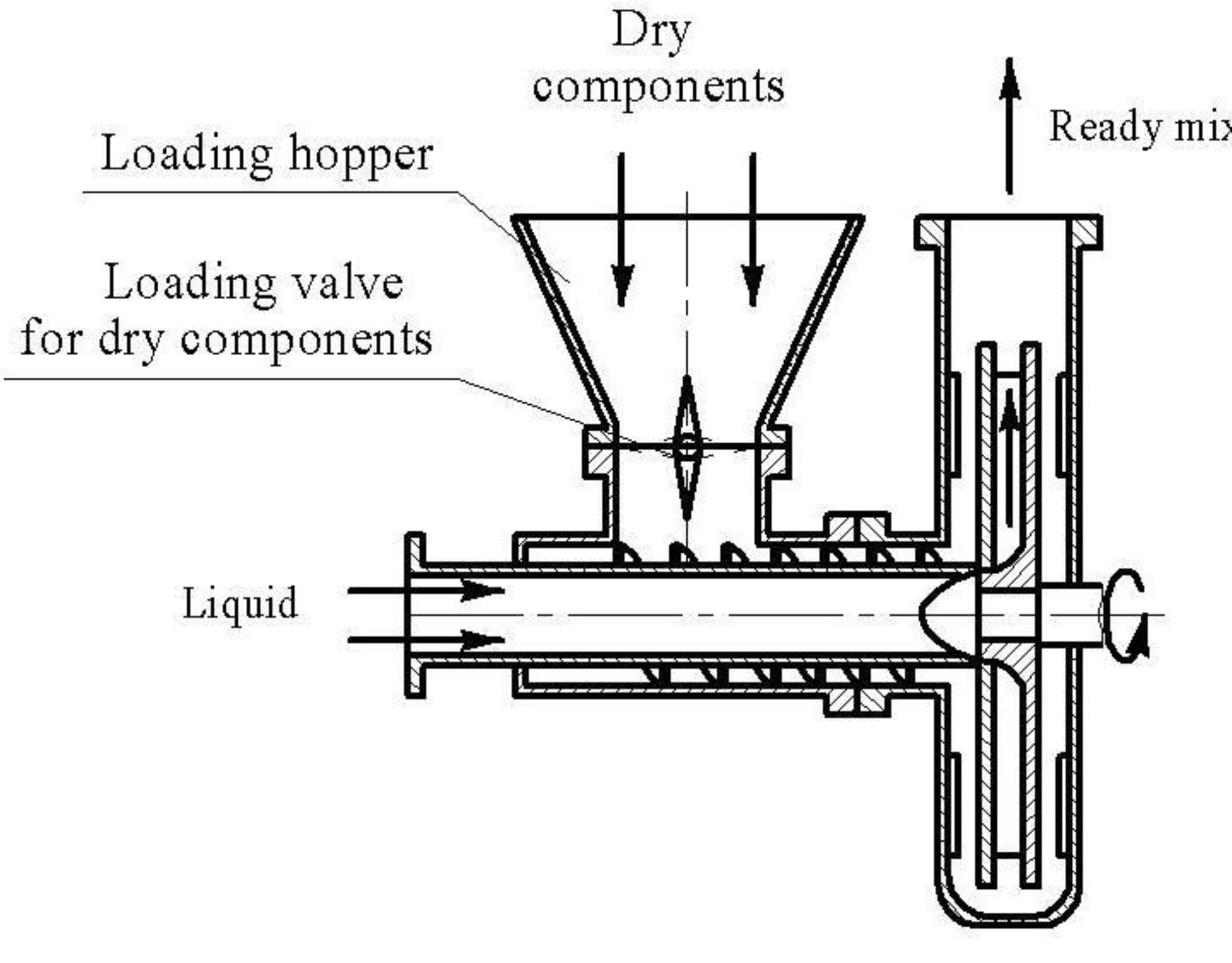
• Modern installations should have versatility in any technological line; for example, the installation, which can not only mix, but further transports the mixture like a conventional pump while providing a dosing device that is necessary to supply dry components.
• When conducting theoretical studies concerning design of the impeller [11,12] we can obtain determination of the size of the modelling of mixing processes.
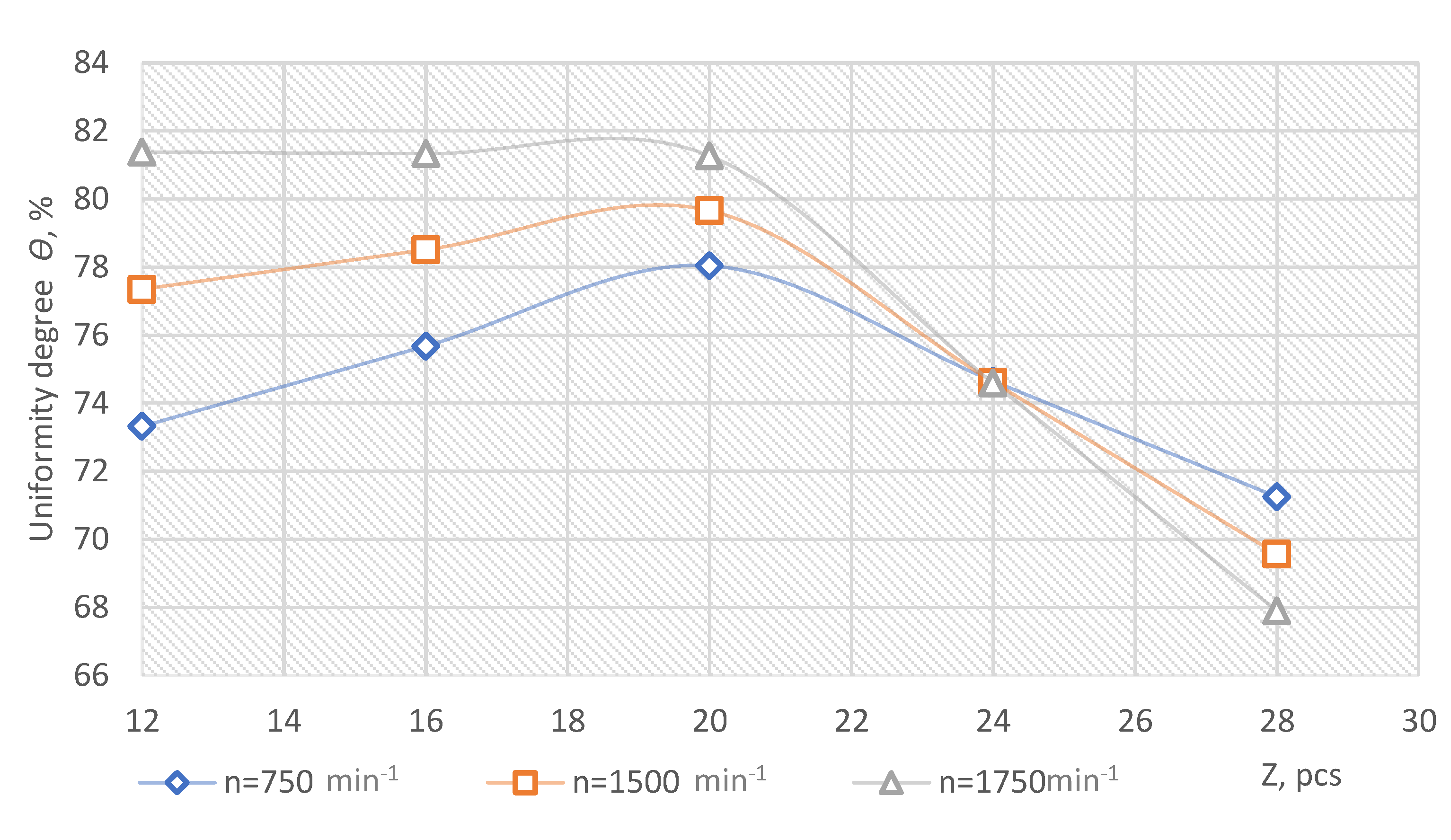
• Experimental studies were carried out to determine the design parameters of the installation in continuous operation. The degree of homogeneity was Θ = 74%, with β2 = 80 … 100° and βst = 65 … 102°, while the value of the consumption of electrical energy is equal Eel = 0.265 … 0.28 kWh/t. The corners can be arranged radially, that is, under the basic values of 90 degrees.

References

1. Rieger, F.; Jirout, T.; Rzyski, E. Mixing of suspensions. Selection of the mixer and tank. Inz. Ap. Chem. 2002, 41, 111–112. (In Polish) [Google Scholar]
2. Grenville, R.K.; Mak, A.T.C.; Brown, D.A.R. Suspension of solid particles in vessels agitated by axial flow impellers. Chem. Eng. Res. Des. 2015, 100, 282–291. [Google Scholar] [CrossRef]
3. Uhl, V.W.; Gray, J.B. Mixing: Theory and Practice; Academic Press: London, UK, 1973; pp. 112–176. [Google Scholar]
4. Nagata, S. Mixing: Principles and Applications; John Wiley & Sons: New York, NY, USA, 1975; pp. 62–65. [Google Scholar]
5. Zlokarnik, M. Stirring: Theory and Practice; Wiley-VCH: Weinheim, Germany, 2001; pp. 76–96. [Google Scholar]
6. Paul, E.L.; Atiemo-Obeng, V.A.; Kresta, S.M. Handbook of Industrial Mixing; John Wiley & Sons: Hoboken, NJ, USA, 2004; pp. 543–584. [Google Scholar]
7. Mak, A.T.C. Solid-Liquid Mixing in Mechanically Agitated Vessels. Ph.D. Thesis, University College London, London, UK, 1992. [Google Scholar]
8. Fort, I.; Jirout, T. A study on blending characteristics of axial flow impellers. Chem. Proc. Eng. 2011, 32, 311–319. [Google Scholar]
9. Джиpyт, T.; Pигep, Φ. Koнcтpyкция кpыльчaтки для пepeмeшивaния cycпeнзий Suspension mixing-impeller design. Chem. Aнгл. Res. Des. 2011, 89, 1144–1151. [Google Scholar]
10. Patuk, I.; Hasegawa, H.; Borodin, I.; Whitaker, A.C.; Borowski, P.F. Simulation for Design and Material Selection of a Deep Placement Fertilizer Applicator for Soybean Cultivation. Open Eng. 2020, 10, 733–743. [Google Scholar] [CrossRef]
11. Patuk, I.; Borowski, P.F. Computer aided engineering design in the development of agricultural implements: A case study for a DPFA. In Journal of Physics: Conference Series; IOP Publishing: Bristol, UK, 2020; Volume 1679, p. 052005. [Google Scholar]
12. Chlebowski, J.; Gaworski, M.; Nowakowski, T.; Szcześniak, A. Effect of liquid feed additive temperature on dosing accuracy in feeding station for dairy cattle. Eng. Rural. Dev. 2020, 19, 1003–1008. [Google Scholar] [CrossRef]
Figure 1. Installation diagram for the preparation of liquid feed mixtures.
Processes 09 02104 g001
Figure 2. Diagram of external forces acting on a particle in the impeller of the experimental setup.
Processes 09 02104 g002
Figure 3. Dependence of the particle motion at a speed of rotation of n = 1500 min−1.
Processes 09 02104 g003
Figure 4. Dependence of the particle motion at a rotation frequency of n = 2250 min−1.
Processes 09 02104 g004
Figure 5. Dependence of particle motion at a rotation frequency of n = 3000 min−1.
Processes 09 02104 g005
Figure 6. Dependence of the particle motion at rotation frequencies n = 1500, 2250 and 3000 min−1.
Processes 09 02104 g006
Figure 7. Scheme of operation of the installation with an open circuit. 1—installation; 2—water tank; 3—a tank with a ready-made mixture; 4—DMK-20 multimeter; 5—frequency converter; 6—component loading valve; 7—loading chamber; 8–12—ball valves.
Processes 09 02104 g007
Figure 8. Dependence of the degree of homogeneity Θ,% on the number of stationary blades Z, pcs, at different speeds at angles β2 = 90° and βst = 90°.
Processes 09 02104 g008
Figure 9. Dependence of the degree of homogeneity Θ,% on the number of stationary blades Z, pcs, at different speeds at angles β2 = 30° and βst = 30°.
Processes 09 02104 g009
Figure 10. Dependence of the degree of homogeneity Θ,% on the number of stationary blades Z, pcs, at different rotational speeds at angles β2 = 150° and βst = 150°.
Processes 09 02104 g010
Figure 11. Two-dimensional section of the response surface of the degree of homogeneity (––––) and the consumption of electrical energy (- - - - -) from the number of blades and the frequency of rotation of the impeller shaft.
Processes 09 02104 g011
Figure 12. Two-dimensional section of the response surface of the degree of homogeneity (––––) and the consumption of electrical energy (- - - - -) from the angles of the impeller and stationary blades.
Processes 09 02104 g012