Synthesis of Cost-Optimal Heat Exchanger Networks Using a Novel Stochastic Algorithm and a Modified Stage-Wised Superstructure

Abstract

Facing the current energy structure urgently needs to be transformed, heat exchanger network (HEN) can implement heat recovery and cost reduction by the arrangement for heat exchanges between cold and hot streams. The plenty of integer and continuous variables involved in HEN synthesis cause the results to be easily trapped in local optima. To avoid this situation, the mechanism of accepting imperfect solutions is added in a novel algorithm called Random Walk Algorithm with Compulsive Evolution. However, several potential solutions maybe abandoned by accepting imperfect solutions. To maintain the global searching ability, and at the same time, protecting the potential solutions during the optimization process, the limitations of accepting imperfect solutions are investigated in this work, then a back substitution strategy and elite optimization strategy based on algorithm are proposed. The former is to identify and adjust the inferior individuals in long-term stagnation while the latter is to keep and perform a fine search for the better solutions. Furthermore, a modified stage-wised superstructure is also developed to implement the flexible placement of utilities, which efficiently enlarges the solution domain. The validation of strategies and model is implemented by three cases, the results are lower, with 2219 $/year, 1280 $/year, and 2M $/year than the best published result, revealing the strong abilities of the proposed method in designing more economical HENs.

1. Introduction

Heat exchanger network (HEN) synthesis can effectively realize heat recovery, reduce external utility consumptions, and improve economic benefits, so it has attracted extensive attention from many academic researchers and engineering workers in the past four decades and is widely applied in various fields including chemical process and crude refining industries [1,2]. HEN synthesis (HENS) is the heat integration between hot and cold process streams [3] with the aim of minimizing total annual cost (TAC) consisting of three sections i.e., utility consumption cost, fixed charge, and area cost of heat units.

Many methodologies for HENS have been developed and they can be broadly split into two categories, thermodynamic approaches and mathematical programming methods [4]. Pinch method [5] is a classical method used to evaluate optimal HEN using thermodynamics laws. In this method, the pinch point is first identified based on the given heat recovery approach temperature to predict maximal heat recovery, then the original HEN is decomposed according to the pinch point to predict minimal heat units. Subsequently, several methods deriving from pinch technology are proposed, including dual-temperature approach [6] and pseudo-pinch design method [7]. The pinch-based methods are well developed and demonstrated excellent efficiency [8,9,10].

Mathematical programming methods mean the formulation and solution of mathematical models, some key developments of which should also be highlighted. In 1983, a linear programming (LP) for the minimization of utility consumptions and a mixed integer linear programming (MILP) for the minimal heat units were formulated in a transshipment model [11] and a transportation model [12]. In 1986, a non-linear programming (NLP) was proposed by Floudas et al. [13] to solve the lowest heat exchanger area cost following the solution of LP and MILP problems. The solution process was substantially sequential, which was similar to pinch technology. The common shortcoming of the sequential methods are the lack of simultaneous consideration for the three-way costs, tending to get suboptimal HENs [14]. Hence, simultaneous methods with mixed integer non-linear programming (MINLP) formulation were proposed and could achieve better HENs than sequential methods [15], the most popular one in which was a stage-wised superstructure (SWS) model proposed by Yee and Grossmann [16]. However, in the SWS model, the utility was only allowed to be placed at the end of streams, limiting the flexible development of structures.

The simultaneous optimization models with MINLP formulation is strongly non-linear and non-convex. The structure optimization related to integer variables is essentially a complex combinatorial problem. Even for a fixed structure, how to obtain optimal distribution of heat exchanger area is a complex non-linear problem with multiple local optimums. Furthermore, Furman and Sahinidis [17] proved that HENS based on MINLP model was non-deterministic polynomial-time hard (NP-hard), so it is difficult to get global optimum even for small cases. Therefore, seeking for efficient global optimization methods to tackle MINLP problems has been the critical issue of HENS. Current methods can be generally classified into deterministic approaches and stochastic approaches [18]. The deterministic approaches [19,20,21] tend to get local optimums. Their computational efficiency decreased exponentially with the increase of problem size [22], indicating an unaccepted computation effort.

Compared with deterministic approaches, stochastic approaches are flexible, efficient, and independent of the initial conditions, which can provide satisfactory results in reasonable time. The stochastic approaches have been widely investigated, including genetic algorithm (GA) [23], simulated annealing (SA) algorithm [24], particle swarm optimization (PSO) [25], differential evolution (DE) algorithm [26], etc. Luo et al. [27] presented a GA considering areas and heat capacity flow rates as genes, so infeasible networks could be avoided. The randomized algorithms had success in uncovering new and better HENs by the random search of the cost landscape, proving that randomization technique can be applied to HEN designs effectively [28,29,30]. A two-level concept [31] consisting of nondeterministic performances has also been developed for HENS, where one level handles the network structures related to integer variables, the other one handles heat loads and spilt ratios related to continuous variables [22,32,33]. Further, Lucas et al. [34] used a two-level meta-heuristic optimization approach involving PSO and SA to optimize work and heat exchange networks. The application of two-level methods improves the HEN results to some extent, but it makes the optimization of integer and continuous variables separate, which can hardly explore the optimal HEN. Recently, GA has been greatly developed in recent years. Feyli et al. [35] combined GA with a technique named modified quasi-linear programming. Their method can get lower TAC of HENs due to the relatively linear behavior of the proposed method. A combined GA [36] method was also used to obtain optimal path of streams inside shell and tube HEs. Thus, the pressure drop of streams can be considered in HENs to reduce pump cost. Furthermore, the stochastic algorithms like GA, PSO, and DE require information exchanges between individuals, which may lead to a certain degree of weakening of the global optimization ability in the later stages of the optimization. To overcome this problem, a novel random walk algorithm with compulsive evolution (RWCE) was presented by Xiao and Cui [37]. In RWCE, individuals executed random walking independently and realized the simultaneous optimization of integer and continuous variables. A simplified Metropolis acceptance rule was also designed to promote structure mutation, which was implemented by accepting imperfect solutions (AIS) with a certain probability. The Metropolis acceptance rule i.e., the AIS behavior was an effective strategy applied to HENS problems [28,33], which was conducive to the local minimum avoidance. However, in RWCE, the AIS may cause individuals to get trapped in long-term evolutionary stagnation with the generation of numerous ineffective random walks, which is a limitation found in substantial case studies. We named this limitation L1. Additionally, AIS may also cause the original solutions before AIS to be replaced by imperfect solutions, so the original solutions cannot be exploited completely, which is another limitation called L2. Due to the two limitations, the RWCE can hardly evolve further and consequently miss the optimum.

The AIS plays a significant role in the applications of stochastic methods to HENS problems, the limitations of which should be investigated to help design better HENs. Therefore, the motivation of this work is to explore the specific limitations of AIS in HENS problems, based on which, two novel strategies including back substitution strategy and elite optimization strategy are proposed respectively to deal with L1 and L2. Then a novel algorithm combining RWCE and the two novel strategies is formed. Moreover, a modified SWS model is also designed with a flexible utility placement strategy, to embed more possible network structures. Finally, the novel algorithm and the modified SWS model are applied for the stream-splitting HENS problems.

In the following parts of the paper, the representation of the modified SWS model and the corresponding mathematical formulation are presented in Section 2, the novel algorithm is described in detail in Section 3, the investigative results of three illustrative cases are presented in Section 4 to verify the effectiveness of the proposed method, finally Section 5 provides the conclusions.

2. Mathematical Formulation and RWCE

The HENS process can be stated as the heat integration between a set of N_H hot streams (to be cooled down to their required temperatures) and a set of N_C cold streams (to be heated up to their required temperatures). The given conditions include heat capacity flow rate of each stream, overall heat transfer coefficients of each potential match, and cost data of heat exchangers and utilities.

A modified SWS (MSWS) model is proposed here, where utilities can be placed at the end of streams and each stream branch, so inner utilities can be obtained. Some similar superstructures can also be seen in the literatures [38,39]. Figure 1 depicts the comparison of SWS and MSWS based on a four-stream problem. Obviously, the MSWS includes the SWS. Moreover, the assumption of non-isothermal mixing [40,41,42] is used here. The simplification of isothermal mixing assumption requires that the outlet temperatures of all branches of a single stream are equal at each stage, which is a limitation to the generation of better candidate HEN structures.

2.1. Objective Function

The objective function of HENS is TAC:

$$\min \mathrm{TAC}={\displaystyle \sum }_{i=1}^{N_{\mathrm{H}}}{\displaystyle \sum }_{j=1}^{N_{\mathrm{C}}}{\displaystyle \sum }_{k=1}^{N_{\mathrm{S}}}\left(C_{\mathrm{F}}{E}_{i,j,k}+C_{\mathrm{A}}{A}_{i,j,k}^{\beta }\right)$$

$$+{\displaystyle \sum }_{i=1}^{N_{\mathrm{H}}}\left(C_{\mathrm{F}}{E}_{\mathrm{CU},i}+C_{\mathrm{A}}{A}_{\mathrm{CU},i}^{\beta }+C_{\mathrm{CU}}{Q}_{\mathrm{CU},i}\right)$$

$$+{\displaystyle \sum }_{j=1}^{N_{\mathrm{C}}}\left(C_{\mathrm{F}}{E}_{\mathrm{HU},j}+C_{\mathrm{A}}{A}_{\mathrm{HU},j}^{\beta }+C_{\mathrm{HU}}{Q}_{\mathrm{HU},j}\right)$$

(1)

$$+{\displaystyle \sum }_{i=1}^{N_{\mathrm{H}}}{\displaystyle \sum }_{j=1}^{N_{\mathrm{C}}}{\displaystyle \sum }_{k=1}^{N_{\mathrm{S}}}\left(C_{\mathrm{F}}{E}_{\mathrm{CU},i,j,k}+C_{\mathrm{A}}{A}_{\mathrm{CU},i,j,k}^{\beta }+C_{\mathrm{CU}}{Q}_{\mathrm{CU},i,j,k}\right)$$

$$+{\displaystyle \sum }_{i=1}^{N_{\mathrm{H}}}{\displaystyle \sum }_{j=1}^{N_{\mathrm{C}}}{\displaystyle \sum }_{k=1}^{N_{\mathrm{S}}}\left(C_{\mathrm{F}}{E}_{\mathrm{HU},i,j,k}+C_{\mathrm{A}}{A}_{\mathrm{HU},i,j,k}^{\beta }+C_{\mathrm{HU}}{Q}_{\mathrm{HU},i,j,k}\right)$$

where $A_{i,j,k}$ is heat exchanger area, $A_{\mathrm{HU},j}$ and $A_{\mathrm{HU},i,j,k}$ are respectively the areas of hot utility at stream end and stream branch, $Q_{\mathrm{HU},j}$ and $Q_{\mathrm{HU},i,j,k}$ are the loads of hot utility respectively at stream end and stream branch. $C_{\mathrm{F}}$, $C_{\mathrm{A}}$, $C_{\mathrm{CU}}$, and $C_{\mathrm{HU}}$ are respectively fixed charge of heat units, area cost coefficient, cost coefficient of cold and hot utility. E is an integer variable representing whether the heat unit exists (E = 1) or not (E = 0).

Areas of heat exchanger can be calculated by Equation (2). Where LMTD represents logarithmic mean temperature difference and is calculated by Equation (5) when ${\theta }_1$ is not equal to ${\theta }_2$, otherwise it is replaced by arithmetic mean temperature difference (AMTD) denned as Equation (6). Where $T_{i,j,k,\mathrm{h}}^{\mathrm{in}}$ and $T_{i,j,k,\mathrm{h}}^{\mathrm{out}}$ are inlet and outlet temperatures of a single exchanger at hot stream; $T_{i,j,k,\mathrm{c}}^{\mathrm{in}}$ and $T_{i,j,k,\mathrm{c}}^{\mathrm{out}}$ are inlet and outlet temperatures of a single exchanger at cold stream. Equation (7) represents the calculation of overall heat exchange coefficient K, where h is individual heat exchange coefficient of streams. The calculation for utility area is similar to Equation (2).

$$A_{i,j,k}=\frac{Q_{i,j,k}}{K_{i,j}LMT{D}_{i,j,k}},i\in N_{\mathrm{H}}, j\in N_{\mathrm{C}}, k\in N_{\mathrm{S}}$$

(2)

$$LMT{D}_{i,j,k}=\frac{\left({\theta }_1-{\theta }_2\right)}{\ln \left({\theta }_1/{\theta }_2\right)},i\in N_{\mathrm{H}}, j\in N_{\mathrm{C}}, k\in N_{\mathrm{S}}$$

(3)

$${\theta }_1=T_{i,j,k,\mathrm{h}}^{\mathrm{in}}-T_{i,j,k,\mathrm{c}}^{\mathrm{out}},i\in N_{\mathrm{H}}, j\in N_{\mathrm{C}}, k\in N_{\mathrm{S}}$$

(4)

$${\theta }_2=T_{i,j,k,\mathrm{h}}^{\mathrm{out}}-T_{i,j,k,\mathrm{c}}^{\mathrm{in}},i\in N_{\mathrm{H}}, j\in N_{\mathrm{C}}, k\in N_{\mathrm{S}}$$

(5)

$$AMT{D}_{i,j,k}=\frac{1}{2}\left({\theta }_1+{\theta }_2\right),i\in N_{\mathrm{H}}, j\in N_{\mathrm{C}}, k\in N_{\mathrm{S}}$$

(6)

$$K_{i,j}=\frac{h_i{h}_j}{h_i+h_j},i\in N_{\mathrm{H}}, j\in N_{\mathrm{C}}$$

(7)

2.2. Constraints

The feasibility constraints are given as follows:

(1) Overall heat balance for each stream

$$(T_i^{\mathrm{in}}-T_i^{\mathrm{out}})\times W_i={\displaystyle \sum }_{k=1}^{N_{\mathrm{S}}}{\displaystyle \sum }_{j=1}^{N_{\mathrm{C}}}{Q}_{i,j,k}+{\displaystyle \sum }_{k=1}^{N_{\mathrm{S}}}{\displaystyle \sum }_{j=1}^{N_{\mathrm{C}}}{Q}_{\mathrm{CU},i,j,k}+Q_{\mathrm{CU},i},i\in N_{\mathrm{H}}$$

(8)

$$(T_j^{\mathrm{out}}-T_j^{\mathrm{in}})\times W_j={\displaystyle \sum }_{k=1}^{N_{\mathrm{S}}}{\displaystyle \sum }_{i=1}^{N_{\mathrm{H}}}{Q}_{i,j,k}+{\displaystyle \sum }_{k=1}^{N_{\mathrm{S}}}{\displaystyle \sum }_{i=1}^{N_{\mathrm{H}}}{Q}_{\mathrm{HU},i,j,k}+Q_{\mathrm{HU},j},i\in N_{\mathrm{C}}$$

(9)

where $T_i^{\mathrm{in}}$ and $T_i^{\mathrm{out}}$ are inlet and outlet temperatures of hot streams; W is heat capacity flow rate.

(2) Heat balance for each heat exchanger

$$(T_{i,j,k,\mathrm{h}}^{\mathrm{in}}-T_{i,j,k,\mathrm{h}}^{\mathrm{out}})\times W_i\times s{p}_{i,j,k,\mathrm{h}}=Q_{i,j,k},i\in N_{\mathrm{H}}, j\in N_{\mathrm{C}}, k\in N_{\mathrm{S}}$$

(10)

$$(T_{i,j,k,\mathrm{c}}^{\mathrm{out}}-T_{i,j,k,\mathrm{c}}^{\mathrm{in}})\times W_j\times s{p}_{i,j,k,c}=Q_{i,j,k},i\in N_{\mathrm{H}}, j\in N_{\mathrm{C}}, k\in N_{\mathrm{S}}$$

(11)

where $s{p}_{i,j,k,\mathrm{h}},$ and $s{p}_{i,j,k,\mathrm{c}}$ are split ratios of hot and cold streams, representing the proportion of the heat capacity flow rate of a stream branch to the corresponding total stream.

(3) Heat balance for each stage

$$\left(T_{i,k}^{\mathrm{out}}-T_{j,k}^{\mathrm{in}}\right)\times W_j={\displaystyle \sum }_{i=1}^{N_{\mathrm{H}}}{Q}_{i,j,k}+{\displaystyle \sum }_{i=1}^{N_{\mathrm{H}}}{Q}_{\mathrm{HU},i,j,k} , jϵN_{\mathrm{C}},kϵN_{\mathrm{S}}$$

(12)

$$\left(T_{j,k}^{\mathrm{out}}-T_{j,k}^{\mathrm{in}}\right)\times W_j={\displaystyle \sum }_{i=1}^{N_{\mathrm{H}}}{Q}_{i,j,k}+{\displaystyle \sum }_{i=1}^{N_{\mathrm{H}}}{Q}_{\mathrm{HU},i,j,k} , jϵN_{\mathrm{C}},kϵN_{\mathrm{S}}$$

(13)

where $T_{i,k}^{\mathrm{out}}$ and $T_{j,k}^{\mathrm{out}}$ are outlet temperatures of hot and cold stream at a certain stage.

(4) Heat balance for the utility at stream branch

$$\left(T_{\mathrm{CU},i,j,k}^{\mathrm{in}}-T_{\mathrm{CU},i,j,k}^{\mathrm{out}}\right)\times W_i\times s{p}_{i,j,k,\mathrm{h}}=Q_{\mathrm{CU},i,j,k} , iϵN_{\mathrm{H}},jϵN_{\mathrm{C}},kϵN_{\mathrm{S}}$$

(14)

$$\left(T_{\mathrm{HU},i,j,k}^{\mathrm{out}}-T_{\mathrm{HU},i,j,k}^{\mathrm{in}}\right)\times W_j\times s{p}_{i,j,k,\mathrm{c}}=Q_{HU,i,j,k} , iϵN_{\mathrm{H}},jϵN_{\mathrm{C}},kϵN_{\mathrm{S}}$$

(15)

where $T_{\mathrm{CU},i,j,k}^{\mathrm{in}}$ and $T_{\mathrm{CU},i,j,k}^{\mathrm{out}}$ respectively denote the inlet and outlet temperatures that a hot stream branch flows through a cold utility, $T_{\mathrm{HU},i,j,k}^{\mathrm{in}}$ and $T_{\mathrm{HU},i,j,k}^{\mathrm{out}}$ respectively denote the inlet and outlet temperatures that a cold stream branch flows through a hot utility.

(5) Heat balance for the utility at stream end

Loads of heat exchangers and inner utilities are treated as optimization variables. If the stream cannot reach the target outlet temperature after each iteration, the utilities at stream end are used as additional energy to meet the requirements.

$$\left(T_{i,NS}^{\mathrm{out}}-T_i^{\mathrm{out}}\right)W_i=Q_{\mathrm{CU},i} , iϵN_{\mathrm{H}}$$

(16)

$$\left(T_{j,1}^{\mathrm{out}}-T_j^{\mathrm{out}}\right)W_j=Q_{\mathrm{HU},i} , jϵN_{\mathrm{C}}$$

(17)

(6) Heat balance for each mixer

$${\displaystyle \sum }_{j=1}^{N_{\mathrm{C}}}(T_{\mathrm{CU},i,j,k}^{\mathrm{out}}\times s{p}_{i,j,k,\mathrm{h}})=T_{i,k}^{\mathrm{out}} , iϵN_{\mathrm{H}}, kϵN_{\mathrm{S}}$$

(18)

$${\displaystyle \sum }_{i=1}^{N_{\mathrm{H}}}(T_{\mathrm{HU},i,j,k}^{\mathrm{out}}\times s{p}_{i,j,k,\mathrm{c}})=T_{j,k}^{\mathrm{out}} , jϵN_{\mathrm{C}}, kϵN_{\mathrm{S}}$$

(19)

(7) Mass balance for each mixer

$${\displaystyle \sum }_{i=1}^{N_{\mathrm{H}}}s{p}_{i,j,k,\mathrm{c}}=1, jϵN_{\mathrm{C}}, kϵN_{\mathrm{S}}$$

(20)

$${\displaystyle \sum }_{j=1}^{N_{\mathrm{C}}}s{p}_{i,j,k,\mathrm{h}}=1, iϵN_{\mathrm{H}}, kϵN_{\mathrm{S}}$$

(21)

(8) Temperature constraints in stream branches

$$T_{i,j,k,\mathrm{h}}^{\mathrm{out}}=T_{\mathrm{CU},i,j,k}^{\mathrm{in}},\hspace{1em}iϵ{\mathrm{N}}_{\mathrm{H}},jϵ{\mathrm{N}}_{\mathrm{C}},kϵ{\mathrm{N}}_{\mathrm{S}}$$

(22)

$$T_{i,j,k,\mathrm{c}}^{\mathrm{out}}=T_{\mathrm{HU},i,j,k}^{\mathrm{in}},\hspace{1em}iϵ{\mathrm{N}}_{\mathrm{H}},jϵ{\mathrm{N}}_{\mathrm{C}},kϵ{\mathrm{N}}_{\mathrm{S}}$$

(23)

(9) Minimum temperature approach constraints

$$T_{i,j,k,\mathrm{h}}^{\mathrm{in}}-T_{i,j,k,\mathrm{c}}^{\mathrm{out}}\ge \Delta T_{\min },iϵ{\mathrm{N}}_{\mathrm{H}},jϵ{\mathrm{N}}_{\mathrm{C}},kϵ{\mathrm{N}}_{\mathrm{S}}$$

(24)

$$T_{i,j,k,\mathrm{h}}^{\mathrm{out}}-T_{i,j,k,\mathrm{c}}^{\mathrm{in}}\ge \Delta T_{\min },iϵ{\mathrm{N}}_{\mathrm{H}},jϵ{\mathrm{N}}_{\mathrm{C}},kϵ{\mathrm{N}}_{\mathrm{S}}$$

(25)

$$T_{\mathrm{CU},i,j,k}^{\mathrm{in}}-T_{\mathrm{CU}}^{\mathrm{out}}\ge \Delta T_{\min },iϵ{\mathrm{N}}_{\mathrm{H}},jϵ{\mathrm{N}}_{\mathrm{C}},kϵ{\mathrm{N}}_{\mathrm{S}}$$

(26)

$$T_{\mathrm{CU},i,j,k}^{\mathrm{out}}-T_{\mathrm{CU}}^{\mathrm{in}}\ge \Delta T_{\min },iϵ{\mathrm{N}}_{\mathrm{H}},jϵ{\mathrm{N}}_{\mathrm{C}},kϵ{\mathrm{N}}_{\mathrm{S}}$$

(27)

$$T_{\mathrm{HU}}^{\mathrm{in}}-T_{\mathrm{HU},i,j,k}^{\mathrm{out}}\ge \Delta T_{\min },iϵ{\mathrm{N}}_{\mathrm{H}},jϵ{\mathrm{N}}_{\mathrm{C}},kϵ{\mathrm{N}}_{\mathrm{S}}$$

(28)

$$T_{\mathrm{HU}}^{\mathrm{out}}-T_{\mathrm{HU},i,j,k}^{\mathrm{in}}\ge \Delta T_{\min },iϵ{\mathrm{N}}_{\mathrm{H}},jϵ{\mathrm{N}}_{\mathrm{C}},kϵ{\mathrm{N}}_{\mathrm{S}}$$

(29)

where $\Delta T_{\min }$ is the minimum approach temperature of heat units. $T_{\mathrm{CU}}^{\mathrm{in}}$ and $T_{\mathrm{CU}}^{\mathrm{out}}$ respectively denote the inlet and outlet temperatures of cold utility. The corresponding symbols for hot utility are $T_{\mathrm{HU}}^{\mathrm{in}}$ and $T_{\mathrm{HU}}^{\mathrm{out}}$.

3. Methodology

A novel algorithm combining RWCE and two strategies to solve the limitations of AIS is designed to solve the complex MSWS model with multiple optimization variables. Several points presented as follows should also be paid attention to. In RWCE, the historical optimum of an individual means the best solution obtained by the individual in the past iterations. The current solution of an individual represents the solution obtained by the individual at the current iteration. The optimal solution indicates the best one in the historical optimums of all the individuals. The optimal TAC after AIS means the best TAC obtained since the individual accepts an imperfect solution at a certain iteration.

3.1. RWCE Method for HENS with Stream Splits

In consideration of MSWS model, an individual in RWCE represents a HEN consisting of heat exchanger loads, inner utility loads, and stream split ratios. The main evolution to implement is the “random walking” of each individual as presented in Equations (30)–(34).

$$Q_{n,p,it+1}^{\prime }=Q_{n,p,it}+\left(1-2\times r_1\right)\times r_2\times S_{\mathrm{Q}},n=1,\dots ,N,p=1,\dots ,NE$$

(30)

$$QIC{U}_{n,l,it+1}^{\prime }=QIC{U}_{n,l,it}+\left(1-2\times r_3\right)\times r_4\times S_{ICU},n=1,\dots ,N,l=1,\dots ,NE$$

(31)

$$QIH{U}_{n,m,it+1}^{\prime }=QIH{U}_{n,m,it}+\left(1-2\times r_5\right)\times r_6\times S_{IHU},n=1,\dots ,N,m=1,\dots ,NE$$

(32)

$$SR{H}_{n,p,it+1}^{\prime }=SR{H}_{n,m,it}+\left(1-2\times r_7\right)\times r_8\times S_{SRH},n=1,\dots ,N,p=1,\dots ,NE$$

(33)

$$SR{C}_{n,p,it+1}^{\prime }=SR{C}_{n,p,it}+\left(1-2\times r_9\right)\times r_{10}\times S_{SRC},n=1,\dots ,N,p=1,\dots ,NE$$

(34)

where $Q_{n,p,it}$ is the initial heat exchanger load, $Q_{n,p,it+1}^{\prime }$ is the heat exchanger load after walking. $QIC{U}_{n,l,it}$ is the initial load of inner cold utility, $QIC{U}_{n,l,it+1}^{\prime }$ is the load of inner cold utility after walking. $SR{H}_{n,m,it}$ represents the initial split ratio of hot stream, $SR{H}_{n,p,it+1}^{\prime }$ is the split ratio of hot stream after walking. $S_q$, $S_{ICU}$, and $S_{IHU}$ are respectively maximal walking step sizes of heat exchanger load, inner cold and hot utilities. $S_{SRH}$ and $S_{SRC}$ are respectively maximal walking step sizes of split ratios of hot and cold streams. $r_1$~$r_{10}.$ are uniform random numbers distributed in the interval (0, 1). Lower bound Q_min is set to handle integer variables to determine the generation and elimination of heat exchangers and inner utilities, which is described as Equation (35) (taking heat exchanger as an example). $Q_{min}$ is a parameter to control the existing of heat exchanger and its value is 10 kW in this paper. If $Q_{n,p,it+1}^{\prime }$ is smaller than $Q_{min}$, the corresponding heat exchanger will be eliminated, making the effective heat exchanger load $Q_{n,p,it+1}^{\prime }$ equal to 0.

$$Q_{n,p,it+1}^{″}=\{\begin{array}{c}{Q}_{n,p,it+1}^{\prime } if Q_{n,p,it+1}^{\prime }\ge Q_{min}\\ 0 else\end{array}$$

(35)

At the $itth$ iteration, the initial solution for individual n can be expressed as $X_{n,it}$. After walking, the new effective solution $X_{n,it+1}^{\prime }$ is generated. Then the TAC($X_{n,it+1}^{\prime }$) is compared with TAC($X_{n,it}$), and the lower one is selected. If TAC($X_{n,it+1}^{\prime }$) is not smaller than TAC($X_{n,it}$), $X_{n,it+1}^{\prime }$ can also be accepted with a certain probability δ. The specific operation is expressed as Equation (36), which is the mutation and selection criterion of RWCE.

$$X_{n,it+1}=\{\begin{array}{c}{X}_{n,it+1}^{\prime } if TAC\left(X_{n,it+1}^{\prime }\right)<TAC\left(X_{n,it}\right)\hfill \\ X_{n,it+1}^{\prime } else if(r_{11}<\sigma )\hfill \\ X_{n,it} else\hfill \end{array}$$

(36)

3.2. Limitations of Accepting Imperfect Solutions

Two limitations of AIS are discussed in this section.

L1: The individuals may not avoid local optimums or even walk to imperfect regions by AIS in the middle or late period, which will lead to the evolution stagnation and efficiency decrease. A nine stream problem listed in

Table 1. Problem data for the case involving nine streams.

Stream	Tin (°C)	Tout (°C)	W (kW/°C)	h (kW/(m2 °C))
H1	327	40	100	0.5
H2	220	160	160	0.4
H3	220	60	60	0.14
H4	160	45	400	0.3
C1	100	300	100	0.35
C2	35	164	70	0.7
C3	85	138	350	0.5
C4	60	170	60	0.14
C5	140	300	200	0.6
HU	330	250	-	0.5
CU	15	30	-	0.5
Annual cost of heat exchangers = 2000 + 70A $/year (A in m2)
Annual cost of hot utility = 60 $/(kW y)
Annual cost of cold utility = 6 $/(kW y)

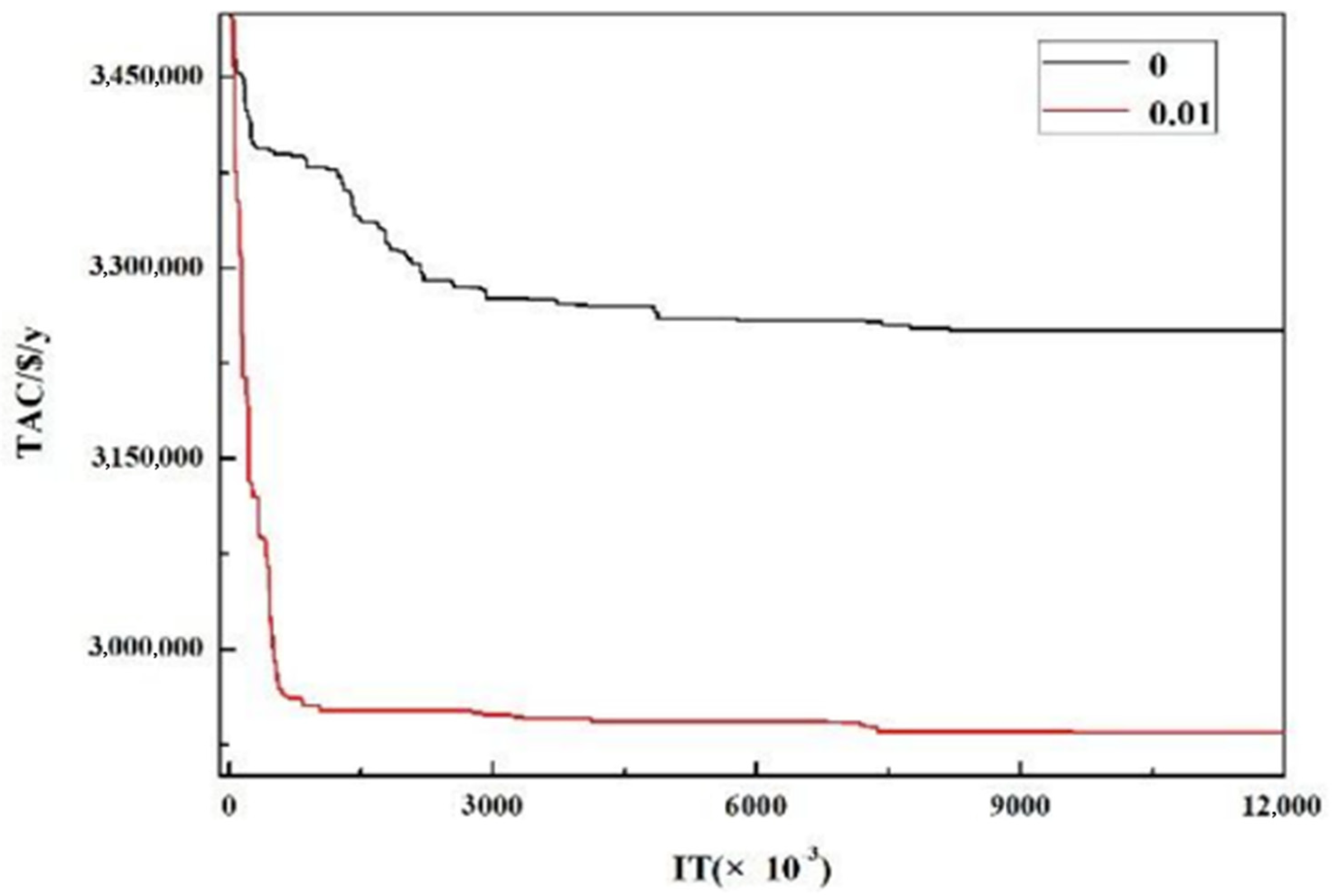
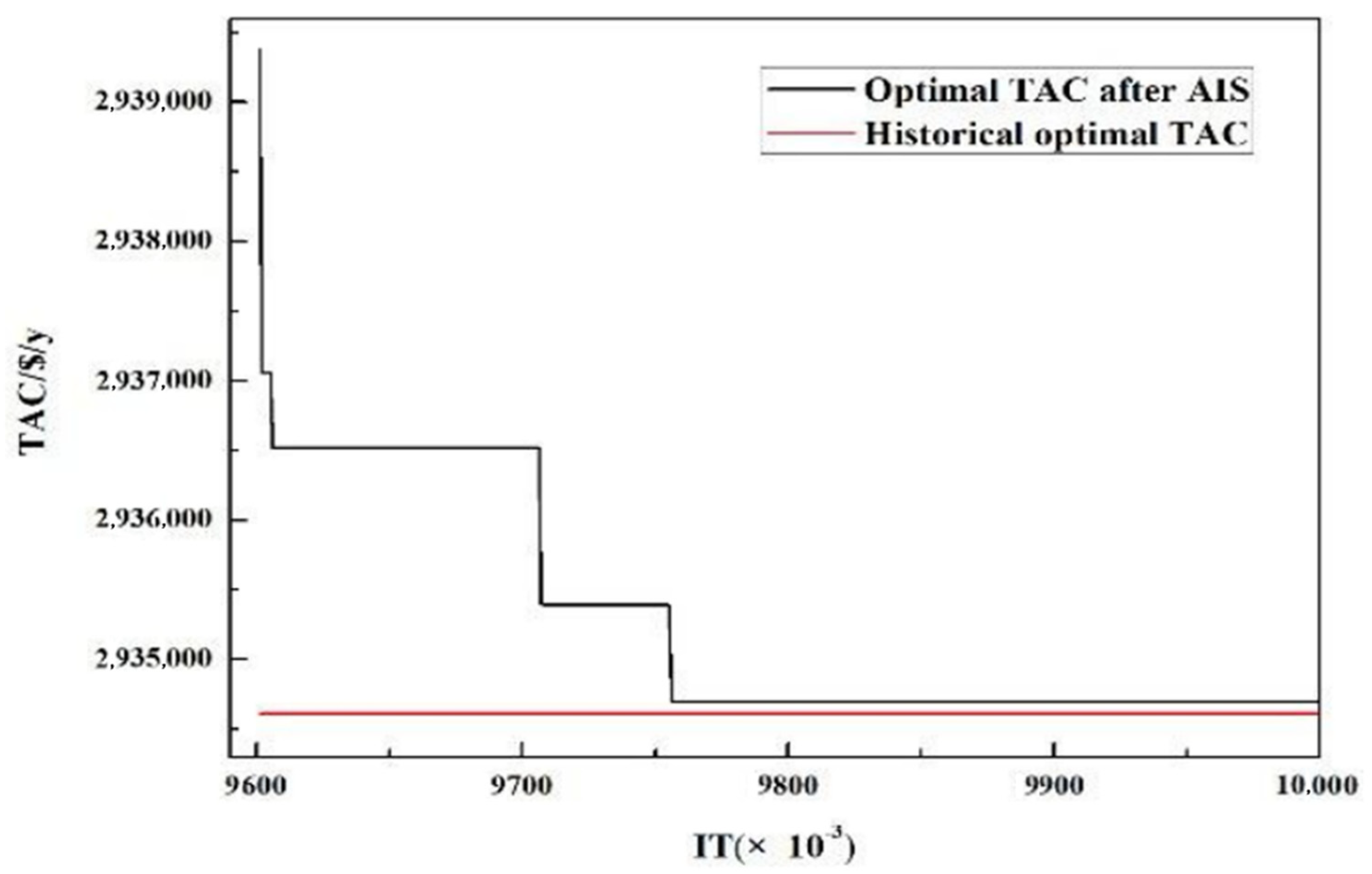
was used to explain the L1. Figure 2 depicts the iteration of optimal TACs obtained by RWCE (N = 1) with the δ respectively set to 0 and 0.01. It is pronounced that the TAC corresponding to δ = 0 declines more slowly compared to that corresponding to δ = 0.01 in the early period. The final TACs corresponding to δ = 0 and δ = 0.01 were respectively 3,250,825 $/year and 2,934,609 $/year, so the AIS could accelerate the evolution process and improve the convergence precision. However, for δ = 0.01, the individual did not evolve (the TAC didn’t decline) any more after about 9,500,000 iterations. By tracking the optimization process, the individual accepted an imperfect solution at the 9,601,186th iteration and the current TAC rose from 2,934,609 $/year to 2,939,384 $/year. Figure 3 displays the iteration of the historical optimal TAC and the optimal TAC after AIS from the 9,601,186th to the 9,999,186th iteration (after the 9,999,186th iteration, the two TACs keep constant). After AIS, the individual could not find better solutions for a long time and stopped at a TAC of 2,934,699 $/year which was inferior to the historical optimal TAC 2,934,609 $/year.

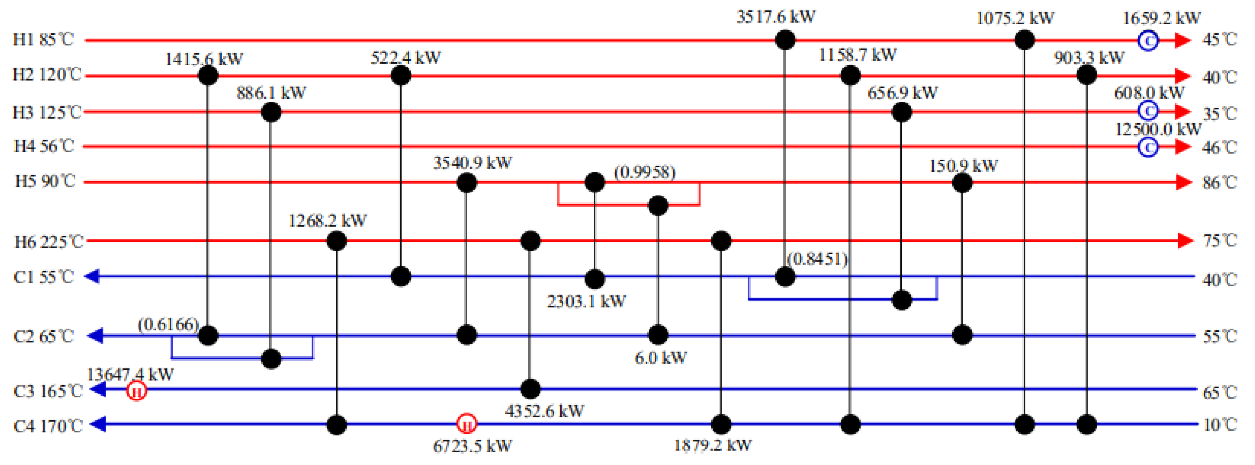
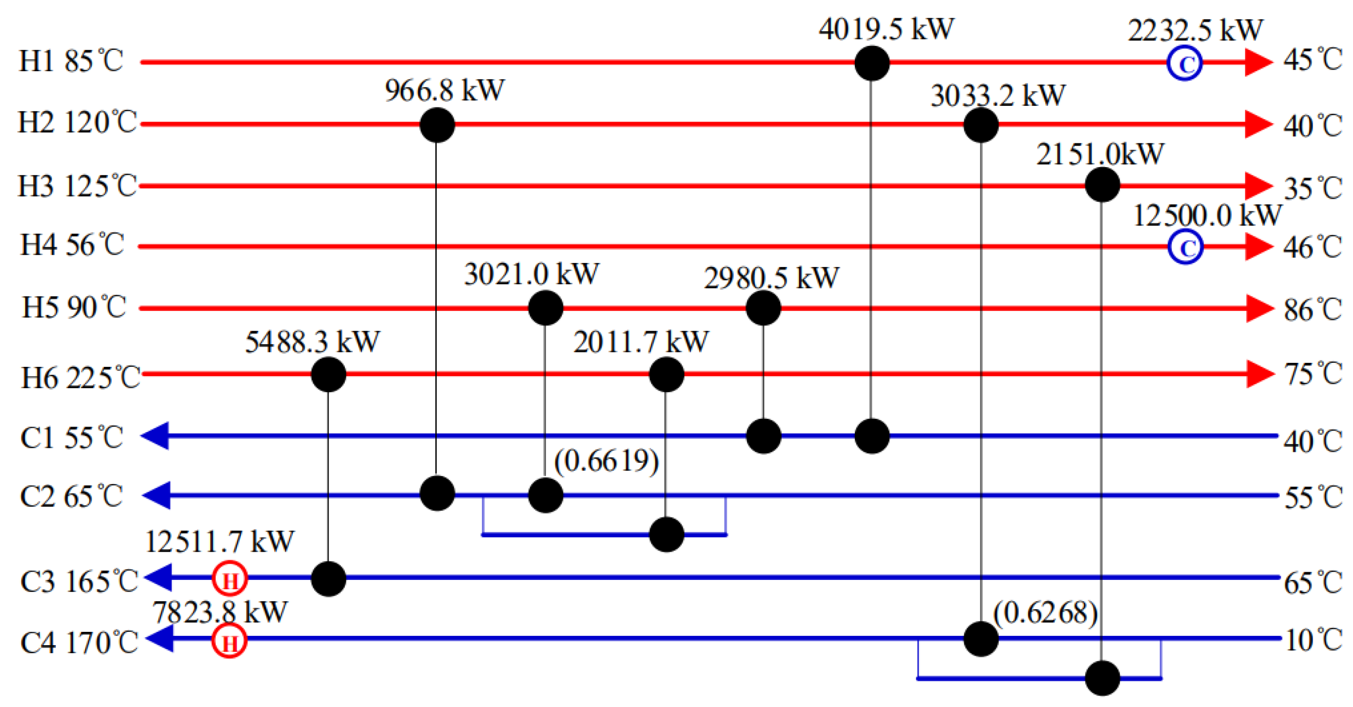
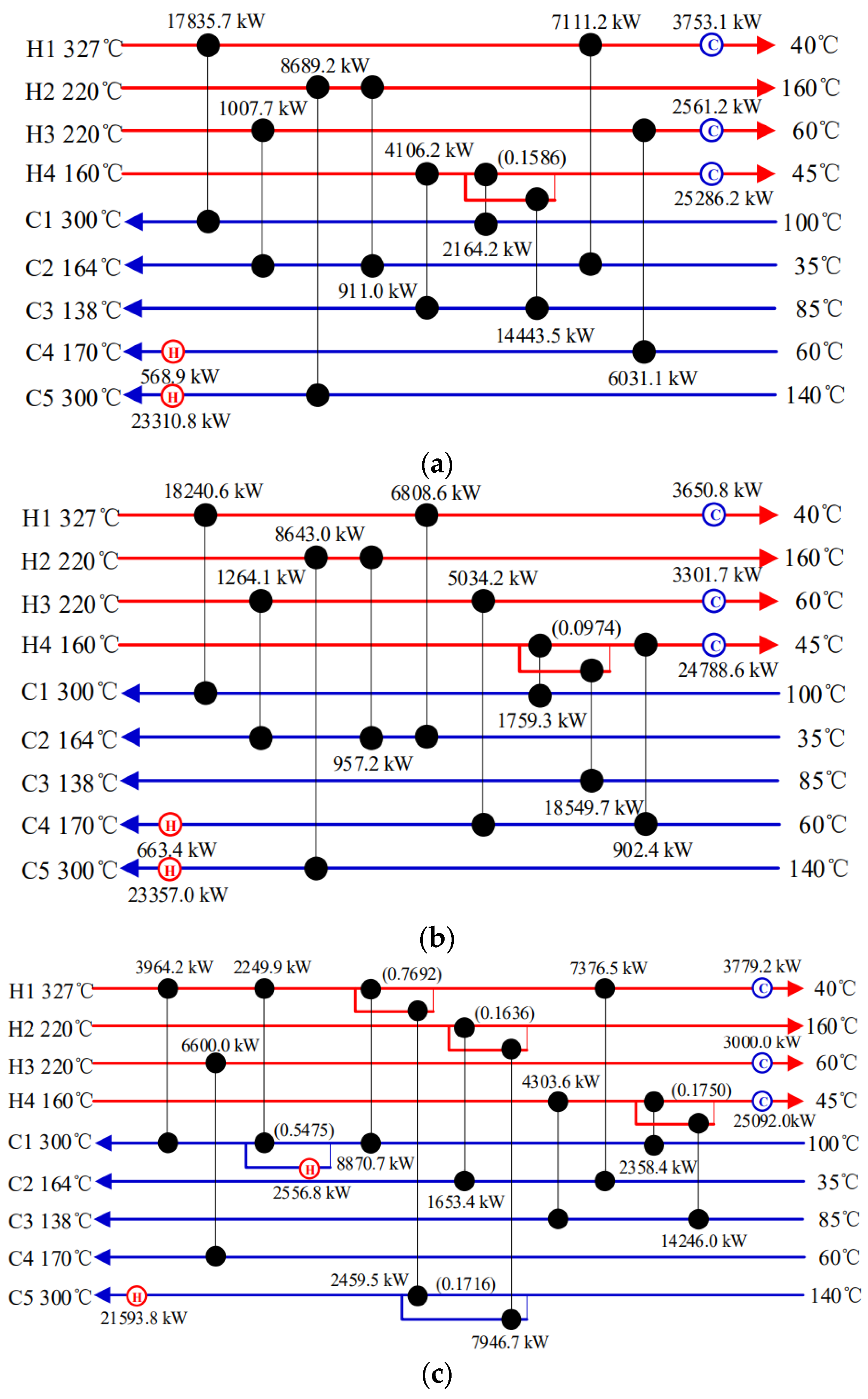
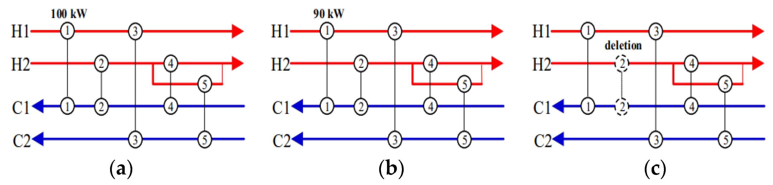
When the individual stopped evolving, its corresponding HEN structure was recorded to compare with its historical optimal structure before AIS. Figure 4 depicts the diagrammatic sketch of the comparison result. Figure 4a shows the best HEN structure before AIS, Figure 4b,c gives possible HEN structures when evolution stops after AIS. It can be found that Figure 4b has the same structure as Figure 4a, but their continuous variables are different. For instance, the heat loads of heat unit 1 in the two structures are respectively 100 kW and 90 kW. While Figure 4c has a structure different from Figure 4a, because the heat unit 2 is deleted in Figure 4c. Therefore, both the continuous variables distribution and the structure might be destroyed after AIS, making the individuals walk ineffectively for a long time and have difficulty in returning to their own best position.

L2: The L2 has a negative effect on the convergence precision, which should also be paid attention to. After accepting an imperfect solution, the original solution before AIS is abandoned that cannot get further optimization, so the original solution is not exploited fully and then the precision declines.

3.3. Strategies

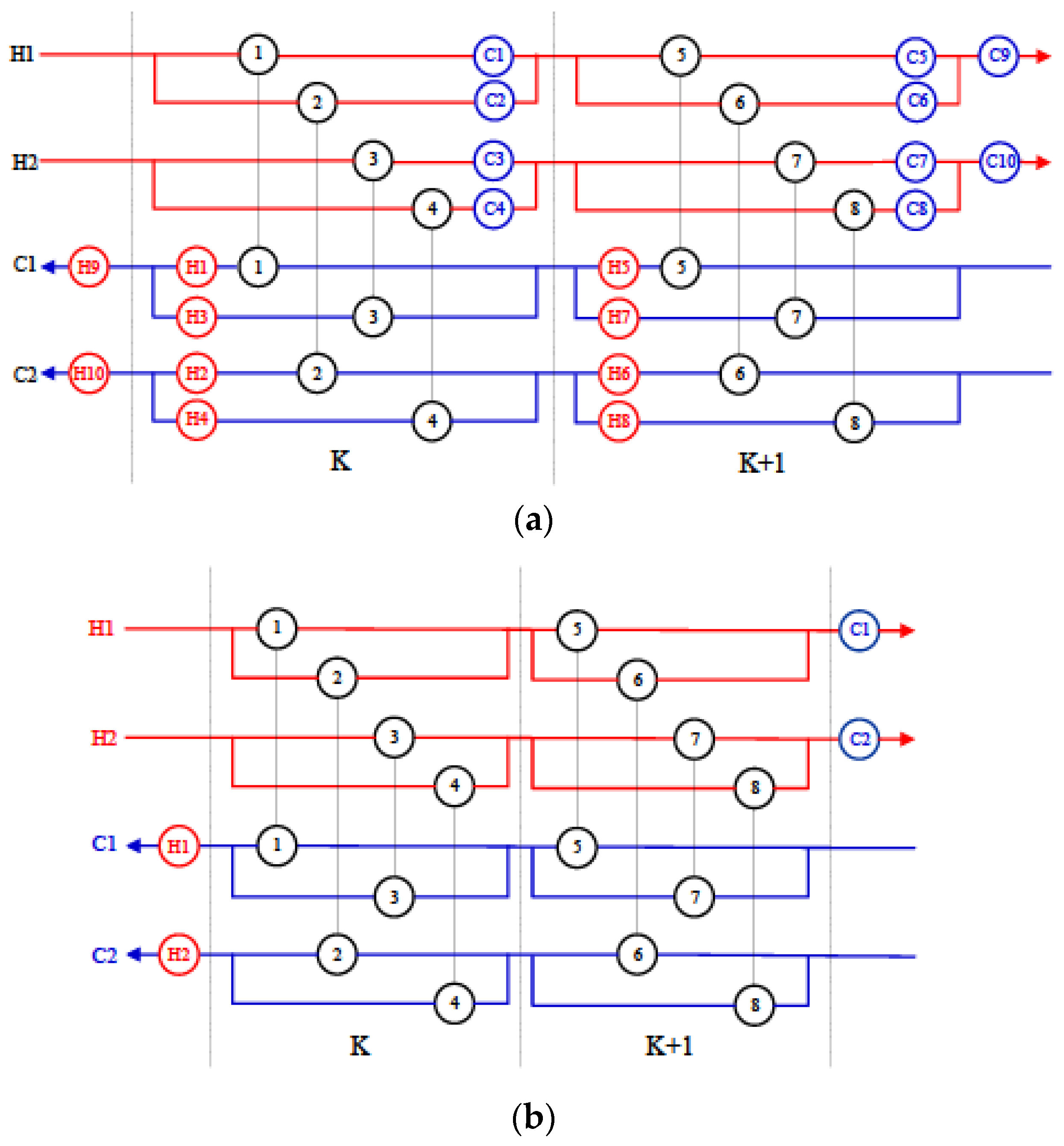
Removing the AIS behavior is obviously an ineffective approach to deal with the two limitations, because it can only keep the local optimums. Therefore, to enhance the search ability of RWCE, two novel strategies aiming at the limitations of AIS are designed in this section. The strategies are then combined with RWCE to form a novel stochastic algorithm named IRWCE.

3.3.1. Back Substitution of Optimums

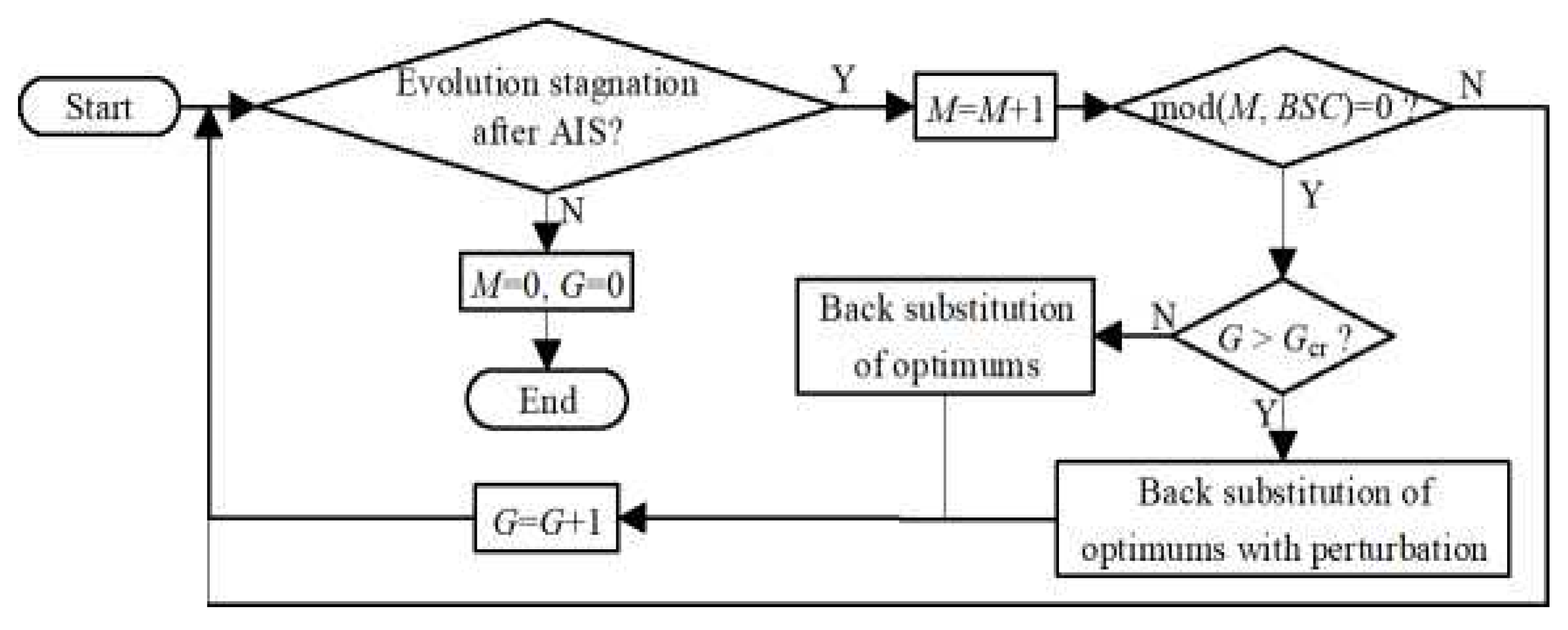
To deal with the L1, a new strategy called back substitution of optimums is developed to compulsively make the individuals in long-term stagnation return to their own historical optimums to adjust their optimization direction in time.

The historical optimum of each individual is first recorded; then an individual condition monitoring mechanism is proposed, a counter is designed to count the evolution stagnation iterations of each individual after AIS. When the individual evolves, the counter resets; when the counter reaches a certain value (BSC), the corresponding individual is considered to be in a long-time stagnation; subsequently, the recorded historical optimum will be delivered to the corresponding individual to implement the back substitution. After back substitution, the count does not continue and becomes zero only if the corresponding individual evolves. If the counter reaches the value 2 × BSC, the back substitution of the recorded historical optimum to the corresponding individual will be performed again. The maximal iteration BSC between two back substitutions is called back substitution cycle. The strategy will be performed repeatedly based on the back substitution cycle if the count continues.

Limited by the relatively small walking step size i.e., $\left(1-2\times r_1\right)\times r_2\times S_Q$, individuals can hardly walk with a long distance in the limited iterations. Hence, when the individual cannot evolve the structure after several operations of back substitution, a random perturbation is executed to achieve a long jump. The perturbation here is described as follows. Some heat loads $Q_{n,best}$ are selected randomly from the individual historical optimal HEN, which are then given perturbation as presented in Equation (37), finally the small heat units are also eliminated as Equation (35). The $r_{12}$ is a uniform random number distributed in the interval (0, 1), k is the perturbation factor. In this study, κ is directly set to 12. The perturbation may help realize long jumps by giving relatively big changes to the heat exchanger loads. However, this perturbation may also destroy the efficient matches of individual historical optimums, so it is executed only when several back substitutions of individual historical optimums cannot evolve the structure.

$$Q_{n,best}^{\prime }=Q_{n,best}\times \kappa {\left(r_{12}-0.5\right)}^2$$

(37)

The working procedure of the back substitution strategy is depicted in Figure 5. The “M” represents the evolution stagnation iterations, “G” is the number of back substitution. The “$G_{cr}$” is set to determine whether the perturbation can be implemented or not.

3.3.2. Elite Optimization

The L2 shows that original solutions before AIS may be replaced by imperfect solutions, so it cannot get complete optimization. Hence, an elite optimization strategy is proposed here to solve L2, where the population is divided into two sections, one section includes NP (NPV0.5N) elite individuals, the other section includes N-NP basic individuals. The elite individuals protect and optimize the solutions with better potentials i.e., elite solutions from being replaced by imperfect solutions, where elite solutions are selected in the optimization process of basic individuals.

The basic individuals evolve as the original RWCE, their historical optimums are sequenced according to TAC, where the top NP historical optimums with relatively lower TACs are selected as the elite solutions and delivered to elite individuals. An elite solution corresponds to an elite individual. If a basic individual updates its historical optimum which is better than the worst elite solution, the new generated optimum will replace the worst elite solution. Thus, the elite solutions are kept without being replaced by imperfect solutions and also have the opportunity to get further optimization.

For the elite solutions, a fine-search (FS) strategy [43] is introduced. The FS strategy can improve the precision in both the continuous and integer variables, which is described in the following. In Equation (38), three logical variables $Z_{n,p}$, $Z_{n,m}$, and $Z_{n,l}$ to determine whether the continuous variables walk ($Z_{n,p}$ = $Z_{n,m}$ = $Z_{n,l}$ = 1) or not ($Z_{n,p}$ = $Z_{n,m}$ = $Z_{n,l}$ = 0) are given. A parameter Φ is set to control the number of variables to evolve. Equations (39)–(43) present the evolution formulation of the elite individuals (the basic individuals use Equations (30)–(34)). The minimal heat load and the AIS probability for the elite individuals are set relatively small to keep the fine search. Figure 6 shows the schematic illustration of the elite optimization strategy.

$$Z_{n,l}=Z_{n,m}=Z_{n,p}=\{\begin{array}{c}1 if r_{13}<\varphi \\ 0 else \end{array}, n=1,\dots ,N, p=1,\dots ,NE, m=1,\dots ,NE, l=1,\dots ,NE$$

(38)

$$Q_{n,p,it+1}^{\prime }=Q_{n,p,it}+\left(1-2\times r_{14}\right)\times r_{15}\times S_Q\times Z_{n,p}, n=1,\dots ,N, p=1,\dots ,NE$$

(39)

$$QIC{U}_{n,l,it+1}^{\prime }=QIC{U}_{n,l,it}+\left(1-2\times r_{16}\right)\times r_{17}\times S_{ICU}\times Z_{n,l} , n=1,\dots ,N,l=1,\dots ,NE$$

(40)

$$QIH{U}_{n,m,it+1}^{\prime }=QIH{U}_{n,m,it}+\left(1-2\times r_{18}\right)\times r_{19}\times S_{IHU}\times Z_{n,m} , n=1,\dots ,N,m=1,\dots ,NE$$

(41)

$$\begin{gathered} SR{H}_{n,p,it+1}^{\prime }=SR{H}_{n,p,it}+\left(1-2\times r_{20}\right)\times r_{21}\times S_{SRH}\times \max \left(Z_{n,p},Z_{n,l}\right), n=1,\dots ,N,p=1,\dots ,NE, \\ l=1,\dots ,NE \end{gathered}$$

(42)

$$\begin{gathered} SR{C}_{n,p,it+1}^{\prime }=SR{C}_{n,p,it}+\left(1-2\times r_{22}\right)\times r_{23}\times S_{SRC}\times \max \left(Z_{n,p},Z_{n,m}\right), n=1,\dots ,N,p=1,\dots ,NE, \\ l=1,\dots ,NE \end{gathered}$$

(43)

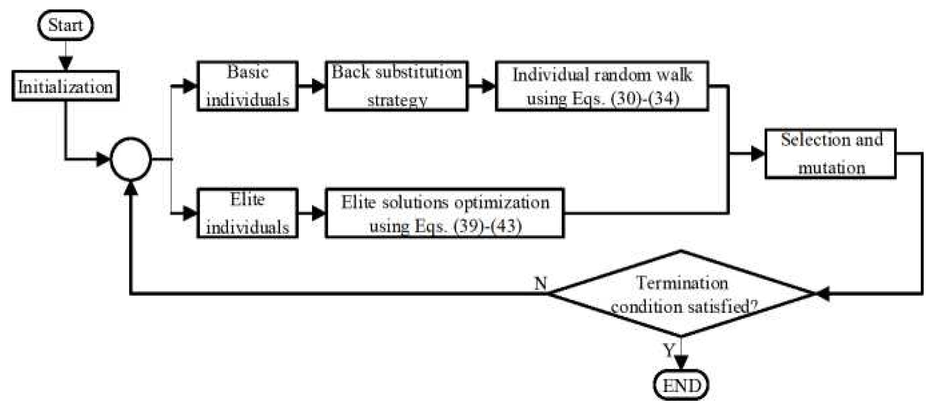
3.4. Calculation Steps of the Improved RWCE

An improved RWCE (IRWCE) based on the original RWCE and the two new strategies is developed, the process of which is exhibited in Figure 7.

(1) Initialization

The population including N-NP basic individuals and NP elite individuals is set. Each individual is initialized as Equations (44)–(48). Where $Q_{n,p,0},QIC{U}_{n,l,0}$, $QIH{U}_{n,m,0}$, $SR{H}_{n,p,0}$, and $SR{C}_{n,p,0}$ respectively represents the initial heat exchanger load, inner cold, and hot utility loads, and split ratios of hot and cold streams; $Q_{max}$, $QIC{U}_{max}$, $QIH{U}_{max }$, $SR{H}_{max}$, and $SR{C}_{max }$ are respectively the initial maximal heat exchanger load, inner cold and hot utility loads, and split ratios of hot and cold streams, they are set as 200 kW, 0 kW, 0 kW, 10 and 10 in this work.

$$Q_{n,p,0}=Q_{max}\times r_{24},n=1,\dots ,N, p=1,\dots ,NE$$

(44)

$$QIC{U}_{n,l,0}=QIC{U}_{max}\times r_{25}$$

(45)

$$QIH{U}_{n,m,0}=QIH{U}_{max}\times r_{26}$$

(46)

$$SR{H}_{n,p,0}=SR{H}_{max}\times r_{27},n=1,\dots ,N, p=1,\dots ,NE$$

(47)

$$SR{C}_{n,p,0}=SR{C}_{max}\times r_{28},n=1,\dots ,N, p=1,\dots ,NE$$

(48)

(2) Back substitution

The back substitution strategy is used for basic individuals. The individual condition monitoring mechanism works to count the evolution stagnation iterations after AIS. If the individuals do not satisfy the requirements of back substitution, this step will be skipped. The strategy is executed based on the back substitution cycle and ends only if the corresponding individual evolves its structure after back substitutions.

(3) Individual random walk

The basic individuals walk according to the Equations (30)–(34), while the elite individuals walk by the Equations (39)–(43). The Equation (35) is used to deal with integer variables, the minimal heat loads for the basic and elite individuals are respectively $Q_{min,b}$ and $Q_{min,e}$.

(4) Selection and mutation

Equation (36) presents the specific implementation of selection and mutation. After random walking, the generated candidate solutions are compared with the initial ones, where the better ones are selected. If the candidate solution is not better than the initial one, the candidate solution will also be accepted with a certain mutation probability. The mutation probabilities for the basic and elite individuals are respectively ${\delta }_b$ and ${\delta }_e$.

(5) Termination

If the maximal iteration is satisfied, the iteration ends; otherwise go to step (2).

4. Results and Discussion

In this section, three different-sized cases available in the literature were solved with the proposed method IRWCE based on the MSWS model. The evaluation for the performance of algorithms depends on the precision and efficiency. While for HENS problems, the precision of the solution obtained within acceptable computation effort is the primary concern [39]. Therefore, the HENs obtained by IRWCE were compared with the previously reported ones on TAC that can describe the optimization precision objectively. The code was implemented using the Compaq Visual Fortran (Version 6.6) and executed on a Windows Server system with an Intel(R) Xeon(R) CPU E31235 @ 3.20 GHz.

4.1. Case Study 1

The case with the problem data listed in

Table 2. Problem data for case 1.

Stream	Tin (°C)	${\mathit{T}}^{\mathbf{out}}$ (°C)	W (kW/K)
H1	85	45	156.3
H2	120	40	50.0
H3	125	35	23.9
H4	56	46	1250
H5	90	86	1500
H6	225	75	50.0
C1	40	55	466.7
C2	55	65	600
C3	65	165	180
C4	10	170	81.3
HU	200	198	-
CU	15	20	-
K = 0.025 kW/(m2 K) for all matches
Annual cost of heat exchangers = 60A $/year (A in m2)
Annual cost of hot utility = 100 $/(kW y)
Annual cost of cold utility = 15 $/(kW y)

have six hot streams and four cold streams. Ravagnani et al. [44] developed a method combining GA and Pinch Method to solve this case, finally a TAC 5,672,821 $/year was presented. The application of IRWCE to the case based on the MSWS model gave a TAC 5,586,395 $/year, the corresponding HEN structure is given in Figure 8 (split ratios are in parentheses).

Table 3. Results comparison for case 1.

Reference	Total Area (m2)	QHU (kW)	QCU (kW)	Units	TAC ($/year)
Ravagnani et al. [44]	56,600.56	20,529.3	14,923.8	13	5,672,821
Huo et al. [45]	57,374	19,991	14,385	13	5,657,000
Huo et al. [45]	57,147	20,000	14,400	13	5,646,000
Huang et al. [40]	56,003.2	20,359.2	14,753.7	18	5,617,431
Khorasany and Fesanghary [22]	58,009.7	19,605.5	14,000	12	5,662,366
Chen et al. [26]	-	20,453	14,847	24	5,588,614
This study (Figure 8)	55,463.42	20,370.95	14,767.26	19	5,586,395

gives the comparison of results; our solution is better than the reported ones and saved 2219 $/year as compared to that by Chen et al. [26]. An inner utility with 6723.5 kW at C4 can be seen in our structure, which cannot be achieved by the original SWS. It indicates that the MSWS enlarges the solution region and can give more satisfactory HEN.

The fixed charge and area cost exponent for the case are respectively zero and one, due to which the obtained HENs tend to include many heat units. To make the case more realistic, Huang et al. [40] provided a new fixed charge 8000 $/year, then they gave a result of 5,737,274 $/year. The modified case was then solved in some literatures. Huang and Karimi [46] gave a HEN with the TAC of 5,733,679 $/year, who used an improved outer-approximation algorithm without generating feasible starting points. Pavao et al. [33] also presented a TAC 5,715,026 $/year by employing a two-level algorithm. In this work, IRWCE and MSWS found a network structure given in Figure 9, its TAC was 5,713,746 $/year and the computational time is 28,810.59 s, which was superior to all the reported ones.

Table 4. Results comparison for case 1 with the fixed charge of 8000 $/year.

Reference	Total Area (m2)	QHU (kW)	QCU (kW)	Units	TAC ($/year)
Huang et al. [40]	56,354.1	20,392.3	14,786.8	12	5,737,274
Wu et al. [42]	-	-	-		5,722,602
Huang and Karimi [46]	56,766.7	20,206.6	14,601.1	11	5,733,679
Pavao et al. [33]	-	-	-	12	5,715,026
This study (Figure 9)	56,053.4	20,335.5	14,732.5	12	5,713,746

presents the results comparison, the significant reduction in area leads to the cost advantage of our solution.

4.2. Case Study 2

The case involving nine streams was further investigated here, which was originally proposed by Linnhoff and Ahmad [47]. The problem data are presented in Table 1. Many scholars tested their methods by solving this case. Huo et al. [45] presented a modified SWS in which the stages with or without stream splits can be determined flexibly, then a two-level algorithm combining GA and PSO was utilized, finally reporting two HENs whose TACs were respectively 2,922,585 $/year and 2,925,634 $/year. Pavao et al. [39] presented a new SWS model with different placements of heaters and coolers, then a modified method combining SA and Rocket Fireworks Optimization was designed and applied to the case, annually giving a TAC 2,909,906 $/year whose structure included an inner utility.

The IRWCE and MSWS were applied to the case, BSC = 2,000,000 was set, then the HEN in Figure 10a was obtained with the TAC of 2,922,234 $/year. When the BSC was set to 3,000,000, a TAC 2,921,233 $/year was obtained, the corresponding structure is presented in Figure 10b. Figure 10c displays the optimal HEN obtained by setting BSC to 2,500,000, whose TAC is 2,907,007 $/year within 8150.20 s and is 2899 $/year less as compared to that by Pavao et al. [39]. The selection of back substitution cycle has significant impact on the optimization process. When BSC is set too big, the individuals in long-term stagnation will not be adjusted in time; when BSC is set too small, the positive effect of AIS will be weakened.

The comparison of results is put in

Table 5. Results comparison for case 2.

Reference	Hot Utility (MW)	Cold Utility (MW)	Units	TAC (M$/year)
Linnhoff and Ahmad [47]	-	-	13	2.930
Luo et al. [27]	23.615	31.335	14	2.922
Chen et al. [26]	23.40	31.12	15	2.924
Lewin [31]	25.09	32.81	12	2.936
Huo et al. [45]	24.58	32.30	11	2.925
Huo et al. [45]	24.22	31.94	13	2.922
Xiao et al. [43]	23.92	31.60	14	2.926
Pavao et al. [33]	23.85	31.57	12	2.919
Pavao et al. [39]	24.76	32.48	14	2.909
This study (Figure 10a)	23.88	31.60	14	2.922
This study (Figure 10b)	24.02	31.74	14	2.921
This study (Figure 10c)	24.15	31.87	16	2.907

. Obviously, our optimal HEN is best, an inner utility (2556.8 kW) can also be seen at a split branch of C1. Furthermore, by observing the temperatures of C1 and HU, the match between C1 and HU is infeasible when C1 is heated to over 250 °C, so the HU at the end of C1 can only be 0 kW (C1 is directly be heated to the target temperature by the matches with hot streams) and over 5000 kW (the outlet temperature of C1 is lower than 250 °C).

4.3. Case Study 3

This is a large scale case including thirteen hot streams and seven cold streams, its data are given in

Table 6. Problem data for case 3.

Stream	Tin (°C)	Tout (°C)	W (kW/K)	h (kW/(m2 K))
H1	576	437	23.1	0.06
H2	599	399	15.22	0.06
H3	530	382	15.15	0.06
H4	449	237	14.76	0.06
H5	368	177	10.7	0.06
H6	121	114	149.6	1.00
H7	202	185	258.2	1.00
H8	185	113	8.38	1.00
H9	140	120	59.89	1.00
H10	69	66	165.79	1.00
H11	120	68	8.74	1.00
H12	67	35	7.62	1.00
H13	1034.5	576	21.3	0.06
C1	123	343	10.61	0.06
C2	20	156	6.65	1.20
C3	156	157	3291	2.00
C4	20	182	26.63	1.20
C5	182	318	31.19	1.20
C6	318	320	4011.83	2.00
C7	322	923.78	17.6	0.06
HU	927	927	-	5.0
CU	9	17	-	1.0
Annual cost of heat exchangers = 4000 + 500A0.83 $/year (A in m2)
Annual cost of hot utility = 250 $/(kW y)
Annual cost of cold utility = 25 $/(kW y)

. Escobar and Trierweiler [48] proposed an initialization strategy to generate better starting points, then they reported a result 1,461,006 $/year that was revised to 1,537,086 $/year by Pavao et al. [25]. Then the later authors provided a TAC 1,516,482 $/y with an improved PSO. By employing the FS strategy, Xiao et al. [43] gave a TAC 1,447,482 $/year.

Applying the proposed method IRWCE and MSWS to the case, a HEN depicted in Figure 11 with the TAC 1,434,297 $/year was obtained, saving 13,185 $/year as compared to the result by Xiao et al. [43]. The computational time of this large-scale case is 28,517.52 s.

Table 7. Results comparison for case 3.

Reference	Total Area (m2)	Qhu (kW)	Qcu (kW)	Units	TAC ($/year)
Escobar and Trierweiler [48]	5551.08	1938.00	106.93	21	1,537,086
Pavao et al. [25]	389.01	1938.00	106.93	21	1,516,482
Xiao et al. [43]	-	867.65	36.6	23	1,447,482
This study (Figure 11)	5412.25	1828.82	0	22	1,434,297

presents the comparison of the results. Obviously, our solution has less utility consumptions and higher precision.

Moreover, an inner hot utility with 825.3 kW is located at C7. Figure 12 gives the comparison of two structures with different utility placement, Figure 12a is the inner utility from Figure 11, Figure 12b is the structure where the utility is moved to the stream end. The two structures have the same heat exchange loads, but total areas in Figure 12a is 286.1 m² less than that in Figure 12b, indicating that the placement of inner utility can help save the areas. In effect, the placement of utility at the stream end reduces the heat exchange temperature difference of the match between HU and C7 and then causes the area to increase from 24.0 m² to 814.9 m².

The parameters of IRWCE used for the three cases are given in

Table 8. Parameters of IRWCE used in this study.

Figure	NS	N	NP	BSC	SQ (SICU,SIHU,KW)	Qmin,b (kW)	${\mathit{Q}}_{\mathit{m}\mathit{i}\mathit{n},\mathit{e} }\left(\mathbf{K}\mathbf{W}\right)$	${\mathit{\delta }}_{\mathit{b}}$	${\mathit{\delta }}_{\mathit{e}}$
Figure 8	6	30	5	2 × 106	80	72	5	0.001	0.0001
Figure 9	6	20	5	3 × 106	80	72	5	0.01	0.0001
Figure 10a	4	50	10	2 × 106	80	72	5	0.001	0.0001
Figure 10b	4	50	10	3 × 106	80	72	5	0.001	0.0001
Figure 10c	4	50	10	2.5 × 106	80	72	5	0.001	0.0001
Figure 11	4	30	15	2 × 106	200	180	5	0.001	0.00001

. Furthermore, for all the three cases, the $S_{SRH}$ and $S_{SRC}$ presented in Equation (48) are set based on whether the corresponding heat exchanger load is zero or not. The values of $\varphi$ for the three cases are respectively given in Equations (49)–(51).

$$S_{SRH}=S_{SRC}=\{\begin{array}{c}0.3 if Q_{i,j,k}=0\\ 0.2 else\end{array}$$

(49)

$$\varphi =\{\begin{array}{c}0.02 if Q_{i,j,k}=0\\ 0.2 else\end{array}$$

(50)

$$\varphi =\{\begin{array}{c}0.01 if Q_{i,j,k}=0\\ 0.15 else\end{array}$$

(51)

$$\varphi =\{\begin{array}{c}0.004 if Q_{i,j,k}=0\\ 0.15 else\end{array}$$

(52)

5. Conclusions

A novel stochastic method IRWCE consisting of RWCE, back substitution strategy, and elite optimization strategy is proposed to solve the HENS problems based on a modified SWS model considering inner utilities. The two novel strategies can maintain the positive effect of AIS and also solve the limitations of AIS, making the IRWCE satisfy the needs of relatively strong global and local search ability. The back substitution strategy is an effective solver of L1, which can deliver the historical optimums to the corresponding individuals in long-term stagnation condition to adjust their evolution direction in time. The elite optimization strategy can deal with L2 by performing a fine search for the selected elite solutions. It was also found that AIS might destroy the efficient structure and continuous variables, significantly influencing the optimization process. The optimal TACs of the three cases obtained by IRWCE were respectively 5,586,395 $/year (5,713,746 $/year when the fixed charge was set to 8000 $/year), 2,907,007 $/year, and 1,434,297 $/y, which saved 2219 $/year (1280 $/year), 2899 $/year, and 13,185 $/year as compared to the reported optimal ones. Some HEN structures with inner utilities were also obtained and significantly reduced the TACs, demonstrating the effectiveness of the MSWS model that enlarged the solution space. The investigative results demonstrated IRWCE and MSWS could achieve better savings in energy consumptions and design cost for HENS problems.

References

1. Kralj, A.K. Optimization of an industrial retrofitted heat exchanger network using a stage-wise model. Energy 2010, 35, 4748–4753. [Google Scholar] [CrossRef]
2. Gadalla, M.A. A new graphical method for Pinch Analysis applications: Heat exchanger network retrofit and energy integration. Energy 2015, 81, 159–174. [Google Scholar] [CrossRef]
3. Angsutorn, N.; Siemanond, K.; Chuvaree, R. Heat Exchanger Network Synthesis using MINLP Stage-wise Model with Pinch Analysis and Relaxation. Comput. Aided Chem. Eng. 2014, 33, 139–144. [Google Scholar] [CrossRef]
4. Salama, A.I.A. Optimization techniques for heat exchanger networks using the minimum rule (MR). Appl. Therm. Eng. 2012, 45, 108–117. [Google Scholar] [CrossRef]
5. Linnhoff, B.; Hindmarsh, E. The pinch design method for heat exchanger networks. Chem. Eng. Sci. 1983, 38, 745–763. [Google Scholar] [CrossRef]
6. Trivedi, K.K.; O’Neill, B.K.; Roach, J.R.; Wood, R.M. A new dual-temperature design method for the synthesis of heat exchanger net-works. Comput. Chem. Eng. 1989, 13, 667–685. [Google Scholar] [CrossRef]
7. Wood, R.M.; Suaysompol, K.; O’Neill, B.K.; Roach, J.R.; Trivedi, K.K. A New Option for Heat Exchanger Network Design. Chem. Eng. Prog. 1991, 87, 38–43. [Google Scholar]
8. Ozkan, S.; Dinger, S. Application for pinch design of heat exchanger networks by use of a computer code employing an im-proved problem algorithm table. Energy Convers. Manag. 2001, 42, 2043–2051. [Google Scholar] [CrossRef]
9. Jiang, N.; Bao, S.; Gao, Z. Heat Exchanger Network Integration Using Diverse Pinch Point and Mathematical Programming. Chem. Eng. Technol. 2011, 34, 985–990. [Google Scholar] [CrossRef]
10. Akbarnia, M.; Amidpour, M.; Shadaram, A. A new approach in pinch technology considering piping costs in total cost target-ing for heat exchanger network. Chem. Eng. Res. Des. 2009, 87, 357–365. [Google Scholar] [CrossRef]
11. Papoulias, S.A.; Grossmann, I.E. A structural optimization approach in process synthesis—II: Heat recovery networks. Comput. Chem. Eng. 1983, 7, 707–721. [Google Scholar] [CrossRef]
12. Cerda, J.; Westerburg, A.W. Synthesizing heat exchanger networks having restricted stream/stream matches using transpor-tation problem formulations. Chem. Eng. Sci. 1983, 38, 1723–1740. [Google Scholar] [CrossRef]
13. Floudas, C.A.; Ciric, A.R.; Grossmann, I.E. Automatic synthesis of optimum heat exchanger network configurations. AIChE J. 1986, 32, 276–290. [Google Scholar] [CrossRef]
14. Xu, Y.-C.; Chen, Q.; Guo, Z.-Y. Entransy dissipation-based constraint for optimization of heat exchanger networks in thermal systems. Energy 2015, 86, 696–708. [Google Scholar] [CrossRef]
15. Ciric, A.R.; Floudas, C.A. Heat exchanger network synthesis without decomposition. Comput. Chem. Eng. 1991, 15, 385–396. [Google Scholar] [CrossRef]
16. Yee, T.F.; Grossmann, I.E. Simultaneous optimization models for heat integration—II. Heat exchanger network synthesis. Comput. Chem. Eng. 1990, 14, 1165–1184. [Google Scholar] [CrossRef]
17. Furman, K.C.; Sahinidis, N.V. Computational complexity of heat exchanger network synthesis. Comput. Chem. Eng. 2001, 25, 1371–1390. [Google Scholar] [CrossRef]
18. Castier, M. Rigorous multiple utility targeting in heat exchanger networks. Energy Convers. Manag. 2012, 59, 74–85. [Google Scholar] [CrossRef]
19. Zamora, J.M.; Grossmann, I.E. A global MINLP optimization algorithm for the synthesis of heat exchanger networks with no stream splits. Comput. Chem. Eng. 1998, 22, 367–384. [Google Scholar] [CrossRef]
20. Ryoo, H.; Sahinidis, N. Global optimization of nonconvex NLPs and MINLPs with applications in process design. Comput. Chem. Eng. 1995, 19, 551–566. [Google Scholar] [CrossRef]
21. Adjiman, C.S.; Androulakis, I.P.; Floudas, C.A. Global optimization of MINLP problems in process synthesis and de-sign. Comput. Chem. Eng. 1997, 21, S445–S450. [Google Scholar] [CrossRef]
22. Khorasany, R.M.; Fesanghary, M. A novel approach for synthesis of cost-optimal heat exchanger networks. Comput. Chem. Eng. 2009, 33, 1363–1370. [Google Scholar] [CrossRef]
23. Dipama, J.; Teyssedou, A.; Sorin, M. Synthesis of heat exchanger networks using genetic algorithms. Appl. Therm. Eng. 2008, 28, 1763–1773. [Google Scholar] [CrossRef]
24. Aguitoni, M.C.; Pavão, L.V.; Ravagnani, M.A.D.S.S. Heat exchanger network synthesis combining Simulated Anneal-ing and Differential Evolution. Energy 2019, 181, 654–664. [Google Scholar] [CrossRef]
25. Pavão, L.V.; Costa, C.B.B.; Ravagnani, M.A.D.S.S. Automated heat exchanger network synthesis by using hybrid natural algo-rithms and parallel processing. Comput. Chem. Eng. 2016, 94, 370–386. [Google Scholar] [CrossRef]
26. Chen, J.; Cui, G.; Duan, H. Multipopulation differential evolution algorithm based on the opposition-based learning for heat exchanger network synthesis. Numer. Heat Transfer. Part A Appl. 2017, 72, 126–140. [Google Scholar] [CrossRef]
27. Luo, X.; Wen, Q.-Y.; Fieg, G. A hybrid genetic algorithm for synthesis of heat exchanger networks. Comput. Chem. Eng. 2009, 33, 1169–1181. [Google Scholar] [CrossRef]
28. Chakraborty, S.; Ghosh, P. Heat exchanger network synthesis: The possibility of randomization. Chem. Eng. J. 1999, 72, 209–216. [Google Scholar] [CrossRef]
29. Pariyani, A.; Gupta, A.; Ghosh, P. Design of heat exchanger networks using randomized algorithm. Comput. Chem. Eng. 2006, 30, 1046–1053. [Google Scholar] [CrossRef]
30. Gupta, A.; Ghosh, P. A randomized algorithm for the efficient synthesis of heat exchanger networks. Comput. Chem. Eng. 2010, 34, 1632–1639. [Google Scholar] [CrossRef]
31. Lewin, D.R. A generalized method for HEN synthesis using stochastic optimization—II: The synthesis of cost-optimal net-works. Comput. Chem. Eng. 1998, 22, 1387–1405. [Google Scholar] [CrossRef]
32. Huo, Z.; Zhao, L.; Yin, H.; Ye, J. A hybrid optimization strategy for simultaneous synthesis of heat exchanger network. Korean J. Chem. Eng. 2012, 29, 1298–1309. [Google Scholar] [CrossRef]
33. Pavao, L.V.; Costa, C.B.B.; Ravagnani, M.A.S.S.; Jiménez, L. Large-scale heat exchanger networks synthesis using simulated anneal-ing and the novel rocket fireworks optimization. AIChE J. 2017, 63, 1582–1601. [Google Scholar] [CrossRef]
34. Santos, L.F.; Costa, C.B.B.; Caballero, J.A.; Ravagnani, M.A.S.S. Synthesis and optimization of work and heat exchanger networks using an MINLP model with a reduced number of decision variables. Appl. Energy 2020, 262, 114441. [Google Scholar] [CrossRef] [Green Version]
35. Feyli, B.; Soltani, H.; Hajimohammadi, R.; Fallahi-Samberana, M.; Eyvazzadeha, A. A reliable approach for heat exchanger networks synthesis with stream split-ting by coupling genetic algorithm with modified quasi-linearprogramming method. Chem. Eng. Sci. 2022, 248, 117140. [Google Scholar] [CrossRef]
36. Sadri, V.; Soltani, H.; Rahimzadeh, S. A Simple Method for Finding Optimal Paths of Hot and Cold Streams inside Shell and Tube Heat Exchangers to Reduce Pumping Cost in Heat Exchanger Network Problems. Chem. Biochem. Eng. Q. 2020, 34, 131–148. [Google Scholar] [CrossRef]
37. Xiao, Y.; Cui, G. A novel Random Walk algorithm with Compulsive Evolution for heat exchanger network synthesis. Appl. Therm. Eng. 2017, 115, 1118–1127. [Google Scholar] [CrossRef]
38. Chen, S.; Cui, G.M. Uniformity factor of temperature difference in heat exchanger networks. Appl. Therm. Eng. 2016, 102, 1366–1373. [Google Scholar] [CrossRef]
39. Pavao, L.V.; Costa, C.B.B.; Ravagnani, M. An enhanced stage-wise superstructure for heat exchanger networks synthesis with new options for heaters and coolers placement. Ind. Eng. Chem. Res. 2018, 57, 2560–2573. [Google Scholar] [CrossRef]
40. Huang, K.F.; Al-mutairi, E.M.; Karimi, I.A. Heat exchanger network synthesis using a stagewise superstructure with non-isothermal mixing. Chem. Eng. Sci. 2012, 73, 30–43. [Google Scholar] [CrossRef]
41. Mujkić, Z.; Ibrić, N.; Bogataj, M.; Kravanja, Z.; Ahmetović, E. Optimisation of heat exchanger networks involving isothermal and non-isothermal mixing by global and local solvers. Comput. Aided Chem. Eng. 2016, 38, 2289–2294. [Google Scholar] [CrossRef]
42. Wu, H.; Yan, F.; Li, W.; Zhang, J. Simultaneous Heat Exchanger Network Synthesis Involving Nonisothermal Mixing Streams with Temperature-Dependent Heat Capacity. Ind. Eng. Chem. Res. 2015, 54, 8979–8987. [Google Scholar] [CrossRef]
43. Xiao, Y.; Cui, G.; Sun, T.; Chen, J. An integrated random walk algorithm with compulsive evolution and fine-search strategy for heat exchanger network synthesis. Appl. Therm. Eng. 2017, 128, 861–876. [Google Scholar] [CrossRef]
44. Ravagnani, M.A.S.S.; Silva, A.P.; Arroyo, P.A.; Constantino, A.A. Heat exchanger network synthesis and optimisation using genetic algo-rithm. Appl. Therm. Eng. 2005, 25, 1003–1017. [Google Scholar] [CrossRef]
45. Huo, Z.; Zhao, L.; Yin, H.; Ye, J. Simultaneous synthesis of structural-constrained heat exchanger networks with and without stream splits. Can. J. Chem. Eng. 2013, 91, 830–842. [Google Scholar]
46. Huang, K.F.; Karimi, I.A. Efficient algorithm for simultaneous synthesis of heat exchanger networks. Chem. Eng. Sci. 2014, 105, 53–68. [Google Scholar] [CrossRef]
47. Linnhoff, B.; Ahmad, S. Cost optimum heat exchanger networks—1. Minimum energy and capital using simple models for capital cost. Comput. Chem. Eng. 1990, 14, 729–750. [Google Scholar] [CrossRef]
48. Escobar, M.; Trierweiler, J.O. Optimal heat exchanger network synthesis: A case study comparison. Appl. Therm. Eng. 2013, 51, 801–826. [Google Scholar] [CrossRef]
Figure 1. Stage-wised superstructure of heat exchanger network. (a) MSWS. (b) SWS.
Processes 09 02060 g001
Figure 2. Iteration of optimal TACs obtained by RWCE with 8 = 0 and 8 = 0.01.
Processes 09 02060 g002
Figure 3. Iteration of the historical optimal TAC and the optimal TAC after AIS.
Processes 09 02060 g003
Figure 4. Possible HENs before and after AIS. (a) The best HEN before AIS. (b) The possible HEN after AIS with different continuous variables. (c) The possible HEN after AIS with different structure.
Processes 09 02060 g004
Figure 5. Working procedure of the back substitution strategy.
Processes 09 02060 g005
Figure 6. The elite optimization strategy.
Processes 09 02060 g006
Figure 7. Diagram of the proposed IRWCE algorithm.
Processes 09 02060 g007
Figure 8. Optimal HEN with the TAC of 5,586,395 $/year for case 1.
Processes 09 02060 g008
Figure 9. Optimal HEN with the TAC of 5,713,746 $/year for case 1 with the fixed charge of 8000 $/year.
Processes 09 02060 g009
Figure 10. Optimal HENs for case 2. (a) The TAC is 2,922,234 $/year. (b) The TAC is 2,921,233 $/year. (c) The TAC is 2,907,007 $/year.
Processes 09 02060 g010
Figure 11. Optimal HEN with the TAC of 1,434,297 $/year for case 3.
Processes 09 02060 g011
Figure 12. Two structures with different utility placement. (a) The inner utility from Figure 11. (b) The utility is located at the stream end.
Processes 09 02060 g012