Multi-Rate Data Fusion for State and Parameter Estimation in (Bio-)Chemical Process Engineering

Abstract

For efficient operation, modern control approaches for biochemical process engineering require information on the states of the process such as temperature, humidity or chemical composition. Those measurement are gathered from a set of sensors which differ with respect to sampling rates and measurement quality. Furthermore, for biochemical processes in particular, analysis of physical samples is necessary, e.g., to infer cellular composition resulting in delayed information. As an alternative for the use of this delayed measurement for control, so-called soft-sensor approaches can be used to fuse delayed multirate measurements with the help of a mathematical process model and provide information on the current state of the process. In this manuscript we present a complete methodology based on cascaded unscented Kalman filters for state estimation from delayed and multi-rate measurements. The approach is demonstrated for two examples, an exothermic chemical reactor and a recently developed model for biopolymer production. The results indicate that the the current state of the systems can be accurately reconstructed and therefore represent a promising tool for further application in advanced model-based control not only of the considered processes but also of related processes.

1. Introduction

In recent years, application of automatic control to bio-chemical manufacturing processes has become increasingly important to keep the required product quality in close bounds, guarantee process safety and also decrease the corresponding environmental impact. Examples are found in a wide range of industries including pharmaceutical and food manufacturing.

For efficient operation, these control approaches require information on the current values of important process states and parameters. Often, those are either corrupted by noise or not directly measurable. Furthermore, measurements of different process quantities are gained from various sensor types which may differ in sampling rate, accuracy and lag. In fact, many online sensors can provide instantaneous but lumped (e.g., mean particle size instead of the full particle size distribution for fluidized bed granulation) or indirect/inferential measurements gained from auxiliary variables (e.g., for drying processes, indirect measurement of product moisture content from moisture content of drying gas at the outlet) [1,2]. In contrast, offline measurements are generally more accurate but accompanied by significant measurement lags, e.g., resulting from sample drawing, preparation and analysis for biochemical processes.

From the control point of view the previously described points lead to a dilemma: On the one hand, fast but rather unreliable data represent no suitable basis for an reliable automatic controller. Though, on the other hand it is also not an option to “wait” for reliable measurement data as corresponding controllers would not be able to act quickly on changes in the process. As an alternative to advanced (and probably too expensive) sensors that allow the generation of accurate and quasi-instantaneous online data, model-based approaches, so-called soft sensors, can be applied to merge different measurements and provide reliable estimates of the current process.

In the literature, this problem has drawn some attention and thus different approaches have been studied. In [3], the most significant estimation algorithms have been presented and compared. Here, Bayesian estimators represent a specific category [4,5,6,7,8] that is an alternative to optimization based techniques such as moving horizon estimators [9,10,11]. An important class of approximative Bayesian estimators are Kalman filters (KF) and particle filters [6,12,13]. In [14] and the references therein, different KF based approaches to the previously stated problem are discussed. Additionally, practical examples of different approaches for (bio-)chemical processes are found in literature, e.g., Kager et al. [15] developed an estimator for penicillin production using online and delayed offline data using particle filtering. The approach showed convincing performance in estimating states and parameters for real measurement data. Furthermore, multi-rate estimators were developed in [16,17,18] estimators were developed and evaluated for pilot-scale polymerization reactors.

In this contribution, we present a new model-based methodology, which is able to merge measurements of various sampling rates, lag horizons and accuracies. The approach is based on cascaded unscented Kalman filters (UKF). Application to two example processes, a nonlinear exothermic reactor and microbial biopolymer production, is demonstrated. The results are discussed and indicate that the presented concept is able to provide reliable online-estimates and is easily adaptable to a wide range of processes.

2. Methods

2.1. Unscented Kalman Filtering

Assume that the process model is given as

$$\begin{array}{cc}\hfill \dot{x}\left(t\right)& =f\left(x\left(t\right),u\left(t\right),w\left(t\right)\right)\hfill \\ \hfill y\left(t\right)& =h\left(x\right(t),u(t),v(t\left)\right)\hfill \end{array}$$

(1)

with $x\in {\mathbb{R}}^{n_x}$, $y\in {\mathbb{R}}^{n_y}$ and $u\in {\mathbb{R}}^{n_u}$ representing the systems state, output and input vector. Furthermore, the systems initial state is denoted as $x_0\in {\mathbb{R}}^{n_x}$. In general, the states dynamics f as well as the measurement equation h are nonlinear functions of the states and the inputs. In many practical cases, not all dynamic states can be measured directly, i.e., $n_x>n_y$, and furthermore, measurements may be corrupted by noise processes $w\left(t\right)$. Moreover, the process dynamics itself may only be known up to a certain degree or be affected by stochastic processes summarized in the signal $v\left(t\right)\in {\mathbb{R}}^{n_v}$.

For state estimation, i.e., the reconstruction of states x from available measurements y, the framework of Kalman filtering can be applied to explicitly account for the underlying noises and uncertainties. In particular for nonlinear dynamics and measurement function, the so-called unscented Kalman filter (UKF) can be applied. The basic formulation as presented in [12,19], is described in a discrete time framework, with systems dynamics and measurement function given by:

$$\begin{array}{cc}\hfill x_k& =f(x_{k-1},u_{k-1})+G_{k-1}{w}_{k-1}\hfill \end{array}$$

(2)

$$\begin{array}{cc}\hfill y_k& =h(x_k,u_k)+v_k\hfill \end{array}$$

(3)

$$\begin{array}{cc}\hfill E\left\{w_k\right\}& =E\left\{v_k\right\}=0\hfill \end{array}$$

(4)

$$\begin{array}{cc}\hfill E\left\{w_k{w}_k^T\right\}& =Q_k,E\left\{v_k{v}_k^T\right\}=R_k\hfill \end{array}$$

(5)

For the sake of simplicity, it is assumed that the process and the measurement noise, $w_k$ and $v_k$, result from random stochastic processes. Without loss of generality, we assume that both can be drawn from zero-mean Gaussian distribution with covariances $Q_k$ and $R_k$. Furthermore, we assume that both affect the states and measurements in an additive sense.

In principle, the traditional structure from the classical Kalman filter [20] for linear dynamics is kept. However, contrarily to the prominent extended Kalman filter (EKF), a sampled-based linearization using Sigma-Points is applied in the UKF. The prediction steps are given as:

• Calculate the Sigma-Points

  $$\begin{array}{cc}\hfill x_{k-1,0}^{(+)}& ={\widehat{x}}_{k-1}^{(+)}\hfill \\ \hfill x_{k-1,i}^{(+)}& ={\widehat{x}}_{k-1}^{(+)}+\sqrt{N+\kappa }{\left(\sqrt{P_{k-1}^{(+)}}\right)}_i^T,i=1,\dots ,N\hfill \\ \hfill x_{k-1,i}^{(+)}& ={\widehat{x}}_{k-1}^{(+)}-\sqrt{N+\kappa }{\left(\sqrt{P_{k-1}^{(+)}}\right)}_i^T,i=N+1,\dots ,2N\hfill \end{array}$$

  (6)
• Propagate each SP using the model equations

  $$\begin{array}{cc}\hfill x_{k,i}^{(-)}& =f\left(x_{k-1,i}^{(+)}\right),i=0,\dots ,2N\hfill \end{array}$$

  (7)
• Using weights

  $$\begin{array}{cc}\hfill w_0& =\frac{\kappa }{N+\kappa }\hfill \\ \hfill w_i& =\frac{1}{2(N+\kappa )},i=1,\dots ,2N\hfill \end{array}$$

  (8)

  determine $P_k^{(-)}$, ${\widehat{x}}_k^{(-)}$, $P_{xy}$, $P_{yy}$ and ${\widehat{y}}_k^{(-)}$ by averaging over weighted SP

  $$\begin{array}{cc}\hfill {\widehat{x}}_k^{(-)}& =\sum _{i=0}^{2N}{w}_i{x}_{k,i}^{(-)},\hfill \end{array}$$

  (9)

  $$\begin{array}{cc}\hfill {\widehat{y}}_k^{(-)}& =\sum _{i=0}^{2N}{w}_i{h}_k\left(x_{k,i}^{(-)}\right),\hfill \end{array}$$

  (10)

  $$\begin{array}{cc}\hfill P_{xy}& =\sum _{i=0}^{2N}{w}_i\left(x_{k,i}^{(-)}-{\widehat{x}}_k^{(-)}\right){\left(h_k\left(x_{k,i}^{(-)}\right)-{\widehat{y}}_k^{(-)}\right)}^T,\hfill \end{array}$$

  (11)

  $$\begin{array}{cc}\hfill P_{yy}& =\sum _{i=0}^{2N}{w}_i\left((h_k\left(x_{k,i}^{(-)}\right)-{\widehat{y}}_k^{(-)}\right){\left(h_k\left(x_{k,i}^{(-)}\right)-{\widehat{y}}_k^{(-)}\right)}^T+R_k,\hfill \end{array}$$

  (12)

  $$\begin{array}{cc}\hfill P_k^{(-)}& =\sum _{i=0}^{2N}{w}_i\left(x_{k,i}^{(-)}-{\widehat{x}}_k^{(-)}\right){\left(x_{k,i}^{(-)}-{\widehat{x}}_k^{(-)}\right)}^T+G_{k-1}{Q}_{k-1}{G}_{k-1}^T.\hfill \end{array}$$

  (13)

Suitable tuning of $\kappa$ is discussed in [12] and the references therein. In the second step, the predicted states and covariance is updated with the current measurement:

$$\begin{array}{cc}\hfill K_k& =P_{xy}·P_{yy}^{-1}\hfill \end{array}$$

(14)

$$\begin{array}{cc}\hfill {\widehat{x}}_k^{(+)}& ={\widehat{x}}_k^{(-)}+K_k\left(y_k-{\widehat{y}}_k^{(-)}\right)\hfill \end{array}$$

(15)

$$\begin{array}{cc}\hfill P_k^{(+)}& =P_k^{(-)}-K_k·P_{yy}·K_k^T\hfill \end{array}$$

(16)

It is worth mentioning, that different extensions and variants have been introduced in the last decades, e.g., the square-root version [12]. Further discussion is provided in [21].

2.2. UKF for Delayed and Multi-Rate Measurements

As described in the introduction, in practice, measurement data is acquired from different sensors that differ not only in accuracy but potentially also measurement delays and sampling rates. The classical formulation presented above must be adapted to such cases in order to allow accurate estimation of states.

In the case of delayed measurements,

$$\begin{array}{c}\hfill y\left(t_k\right)=h(x(t-\tau ),u(t-\tau )),\end{array}$$

(17)

the UKF algorithm is adapted, such that only states up to $\left(t-\tau \right)$ can be reconstructed at the current sample time t. For the interval $\left(t-\tau ,t\right]$ states (and also covariances representing uncertainties) could be predicted using the unscented transformation, i.e., the prediction step of the UKF.

Further adaption is necessary if measurements differ in their respective sampling rates. In the case of two different sensors, a “fast” and a “slow” sensor, the first can be assumed to have sampling rate $\Delta t$ without loss of generality while the sampling rate of the second is given as an integer multiple $N\Delta t$. This means, that the slow measurement is only available for each $N\Delta t$ and the measurement equation therefore is given as:

$$\begin{array}{c}\hfill y_k=\left\{\begin{array}{cc}{\left[y_{k,fast},y_{k,slow}\right]}^T,& \mathrm{if}k=N\Delta t,N\in \mathbb{N}\\ y_{k,fast},& \mathrm{else}\end{array}\right.\end{array}$$

(18)

Obviously, for further sensors, this representation can become rather confusing. Alternatively, in particular in the Kalman Filtering context, it is convenient to keep the standard measurement equation, i.e.,

$$\begin{array}{c}\hfill y_k={\left[y_{k,fast},y_{k,slow}\right]}^T\end{array}$$

(19)

and use a specific weighting of the measurements in the update step by setting high values for the measurement noise of currently not available measurements in the update step.

$$\begin{array}{c}\hfill R_k=\left[\begin{array}{cc}{R}_{k,fast}& 0\\ 0& R_{k,slow}\end{array}\right],R_{k,slow}=\left\{\begin{array}{cc}{R}_{k,slow}^{II},& \mathrm{if}k=N\Delta t,\dots \\ R_{k,slow}^I,& \mathrm{else}\end{array}\right.,R_{k,slow}^I\gg R_{k,slow}^{II}\end{array}$$

(20)

This alternative solution is easier to implement for more than two sensors because the native KF structure can be kept.

An example is given in the following. Assume that a fast sensor has a sampling rate of $\Delta t$ and the slow sensor a sampling rate of $2\Delta t$. This means that $y_{k,slow}$ can only be measured in each second time step and $y_{k,fast}$ in each time step. Thus, the reconstruction of states is alternately based on the measurement of $y_{k,fast}$ and the measurements from both sensors, $y_{k,slow}$ and $y_{k,fast}$, from step to step. In result the measurement equation is given as:

$$\begin{array}{c}\hfill y_k=y_{k,fast},\mathrm{if}k=1,3,5,\dots \\ \hfill y_k={\left[y_{k,fast},y_{k,slow}\right]}^T,\mathrm{if}k=2,4,6,\dots \end{array}$$

(21)

Alternatively, the standard measurement equation, i.e.,

$$\begin{array}{c}\hfill y_k={\left[y_{k,fast},y_{k,slow}\right]}^T\end{array}$$

(22)

is kept with a specific weighting:

$$\begin{array}{c}\hfill R_k=\left[\begin{array}{cc}{R}_{k,fast}& 0\\ 0& R_{k,slow}\end{array}\right],R_{k,slow}=\left\{\begin{array}{cc}{R}_{k,slow}^I,& \mathrm{if}k=1,3,5,\dots \\ R_{k,slow}^{II},& \mathrm{else}\end{array}\right.,R_{k,slow}^I\gg R_{k,slow}^{II}.\end{array}$$

(23)

3. Results and Discussion

This section evaluates the presented methods’ performance to infer the systems state from (potentially) delayed measurements with different sampling rates. Therefore, two examples are analyzed: In the first case, the UKF is applied to a exothermic reactor described by a system of two nonlinear ODEs [22]. In addition to reconstruction of immeasurable states, the UKF’s potential for online parameter estimation is assessed. The second example is concerned with state estimation for microbial-based production of biopolymers in lab-scale setup. The underlying model was recently developed in our group with own experimental data [23].

3.1. Exothermal Chemical Reactor

3.1.1. Model Formulation

The dimensionless model suggested by Schaffner and Zeitz [22] describes the nonlinear dynamics of an exothermic chemical reaction in terms of conversion $x_1$ and temperature $x_2$

$$\begin{array}{cc}\hfill \frac{\mathrm{d}{x}_1}{\mathrm{d}t}& =-a_1{x}_1+{10}^{14}{b}_{1}r(x_1,x_2),\hfill \\ \hfill \frac{\mathrm{d}{x}_2}{\mathrm{d}t}& =-a_2{x}_2+{10}^{14}{b}_{2}r(x_1,x_2)+gu,\hfill \\ \hfill r(x_1,x_2)& =\left(1-x_1\right)exp\left(-\frac{E}{1+x_2}\right).\hfill \end{array}$$

(24)

The control input u represents the heating/cooling of the reactor. Depending on u, the reactor dynamics may exhibit persistent oscillations. Additionally, this model has served frequently as a benchmark in engineering education for the design of nonlinear observers and controllers, where one usually assumes that the temperature is measurable while the conversion is not. However, reconstruction of the conversion from temperature measurements is possible with convenient approaches, e.g., UKF.

In the following, we will assume that measurements of $x_1$ and $x_2$ are available at different sampling rates: While the temperature can be measured rather easily, e.g., with a standard industrial thermometer, direct measurement of conversion would be based on physical samples. Sample analysis may take a certain time span $\tau =k_{del}\Delta t$. The corresponding measurement rate is thus not only possible at a lower rate but also delayed. In terms of a measurement equation this reads as:

$$\begin{array}{c}\hfill y_k=\left[\begin{array}{c}{x}_{(k-k_{del}),1}\\ x_{k,2}\end{array}\right]+\left[\begin{array}{c}{v}_{k,1}\\ v_{k,2}\end{array}\right],E\left\{v_k\right\}=R_k\end{array}$$

(25)

with $y_k=y(t=k\Delta t)$. Following the convention introduced in the previous section, the noise variance of conversion measurements depend on the sampling time:

$$\begin{array}{c}\hfill R_1\left(k\right)=\left\{\left[\begin{array}{cc}{R}_{k,1}^I,& \mathrm{for}k=n{k}_{\mathit{del}},n\in \mathbb{N}\\ R_{k,2}^{II},& \mathrm{else}\end{array}\right]\right..\end{array}$$

(26)

All model parameters can be found in

Table 1. Parameter values for nonlinear reactor model.

Parameter	Value	Parameter	Value
$a_1$	$0.2674$	$a_2$	$1.815$
$b_1$	$1.05$	$b_2$	$0.492$
g	$1.5476$	E	$34.2583$
u	$-0.002$	$\Delta t$	$0.666$
$x_1\left(0\right)$	$0.3$	$x_2\left(0\right)$	$0.1$

. For the simulations an additional unknown stochastic part in the process dynamics was assumed. The deterministic part was solved with the MATLAB function ode15s and for the stochastic part the Euler–Maruyama method [24] was implemented. For the shown scenarios, artificial measurements are used.

3.1.2. Scenario I: State Estimation

In Figure 1 and Figure 2 the performance of the UKF for reconstruction of the states is presented for different time points. UKF parameters and initial conditions are summarized in

Table 2. Parameters and initial conditions for exothermic reactor scenario I.

Parameter	Value	Parameter	Value
${\widehat{x}}_1\left(0\right)$	$0.15$	${\widehat{x}}_2\left(0\right)$	$0.15$
$k_{del}$	10	$\kappa$	1
$R_k^I$	${10}^{-5}\left[\begin{array}{cc}0.5& 0\\ 0& 5\end{array}\right]$	$R_k^{II}$	$\left[\begin{array}{cc}{10}^{15}& 0\\ 0& 5·{10}^{-5}\end{array}\right]$
$P_0^{(-)}$	${10}^{-2}\left[\begin{array}{cc}0.25& 0\\ 0& 0.25\end{array}\right]$	$Q_k$	${10}^{-5}\left[\begin{array}{cc}5& 0\\ 0& 1\end{array}\right]$

.

In the figures, the so-called delay window is denoted with green lines: the right green line denotes the current sampling instant t while the left corresponds to $(t-\tau )$. Within the delay window only the online measurement of the temperature $x_1$ is available but no information is provided for the slow conversion. Thus, state estimates between the two green lines, i.e., $\left(t-\tau ,t\right]$, are only based on temperature measurements. In contrast, state estimates outside of the delay window, i.e., $t\le (t-\tau )$ (left of the green line), are based on measurement of temperature and conversion. In Figure 1 estimation results are shown for two different time points.

A general effect is observed: If a conversion measurement becomes available (black diamond), the estimation accuracy does not only improve significantly for $x_1$ itself but also for $x_2$ as estimation quality of the latter in the delay window crucially depends on the quality of estimates at the left border of the delay window. The slow conversion sensor based update thereby improves estimation accuracy for temperature within the delay window. In Figure 2 the overall estimation results are depicted.

It can be seen that both states are estimated quite accurately in face of the stochastic dynamics and measurements. However, reconstruction of $x_1$ generally becomes worse the longer the time since the last slow sensor measurement and also in the delay window, where estimation is based on measurements of $x_2$ alone.

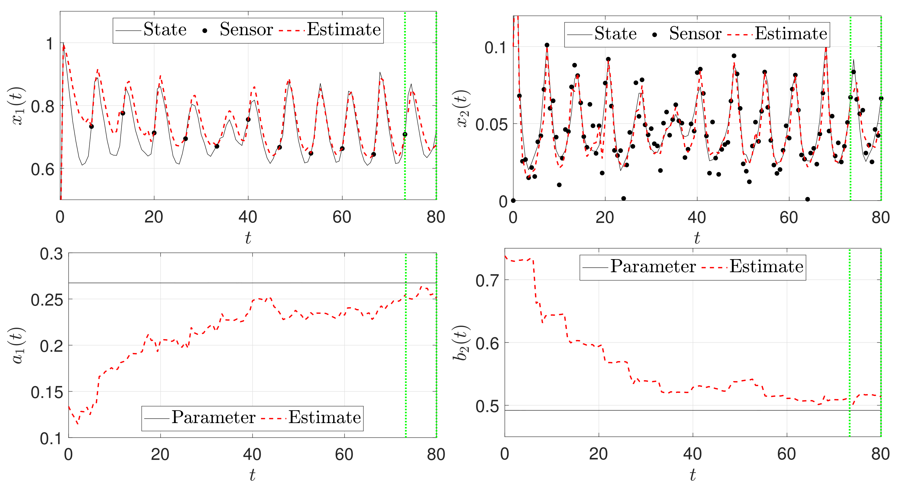
3.1.3. Scenario II: Simultaneous State and Parameter Estimation

In addition to states that cannot be directly measured at each time instance, in practice it frequently occurs that model parameters are either not fully known or even change during process operation, e.g., as a result of aging or fouling processes. In this case, the state estimation problem can be adapted to enable simultaneous estimation of states and parameters.

For the nonlinear reactor the state vector is augmented by the unknown parameters $a_1$ and $b_2$ and the UKF approach is implemented for the augmented state vector

$$\begin{array}{c}\hfill x_{aug}={\left[\begin{array}{c}x,a_1,b_2\end{array}\right]}^T.\end{array}$$

(27)

Initial conditions and further parameters are summarized in

Table 3. Parameters and initial conditions for exothermic reactor scenario II.

Parameter	Value	Parameter	Value
${\widehat{x}}_1\left(0\right)$	$0.3$	${\widehat{x}}_2\left(0\right)$	$0.1$
${\widehat{a}}_1\left(0\right)$	$0.5·a_1$	${\widehat{b}}_2\left(0\right)$	$1.5·b_2$
$k_{del}$	10	$\kappa$	0
$R_k^I$	$\left[\begin{array}{cc}5·{10}^9& 0\\ 0& 1·{10}^{-4}\end{array}\right]$	$R_k^{II}$	$\left[\begin{array}{cc}5·{10}^{-6}& 0\\ 0& 1·{10}^{-4}& \end{array}\right]$
$P_0^{(-)}$	${10}^{-3}\left[\begin{array}{cccc}2.5& 0& 0& 0\\ 0& 2.5& 0& 0\\ 0& 0& 2.5& 0\\ 0& 0& 0& 2.5\end{array}\right]$	$Q_k$	${10}^{-3}\left[\begin{array}{cccc}0.02& 0& 0& 0\\ 0& 0.01& 0& 0\\ 0& 0& 0.025& 0\\ 0& 0& 0& 0.025\end{array}\right]$

.

In the simulations it was assumed that the initial estimates for the kinetic parameters are given as:

$$\begin{array}{c}\hfill {\widehat{a}}_1(t=0)=0.5a_1,{\widehat{b}}_2(t=0)=1.5b_2.\end{array}$$

(28)

The results are depicted in Figure 3.

While estimation of $x_1$ is not sufficient because of inaccurate parameter estimates, slow sensor measurements improve estimation for a certain time span. However, the minima of the oscillations are not well captured for $t<40$. Afterwards, parameter estimates seem to be reasonably close to the process value such that the reconstruction improves. In particular for $b_2$ significant adaption is seen when slow sensor measurements become available. It was also generally observed that estimation of $b_2$ within the delay window is rather inaccurate while for $a_1$ correct trends were seen. The major reason is potentially related to the practical observability: Within the delay window the approach aims on reconstruction of the augmented states from noisy measurement information of $x_2$ alone. In contrast, when a slow sensor measurement becomes available, the additional accurate information on $x_1$ obviously improves the methods potential for estimation of all four variables of interest.

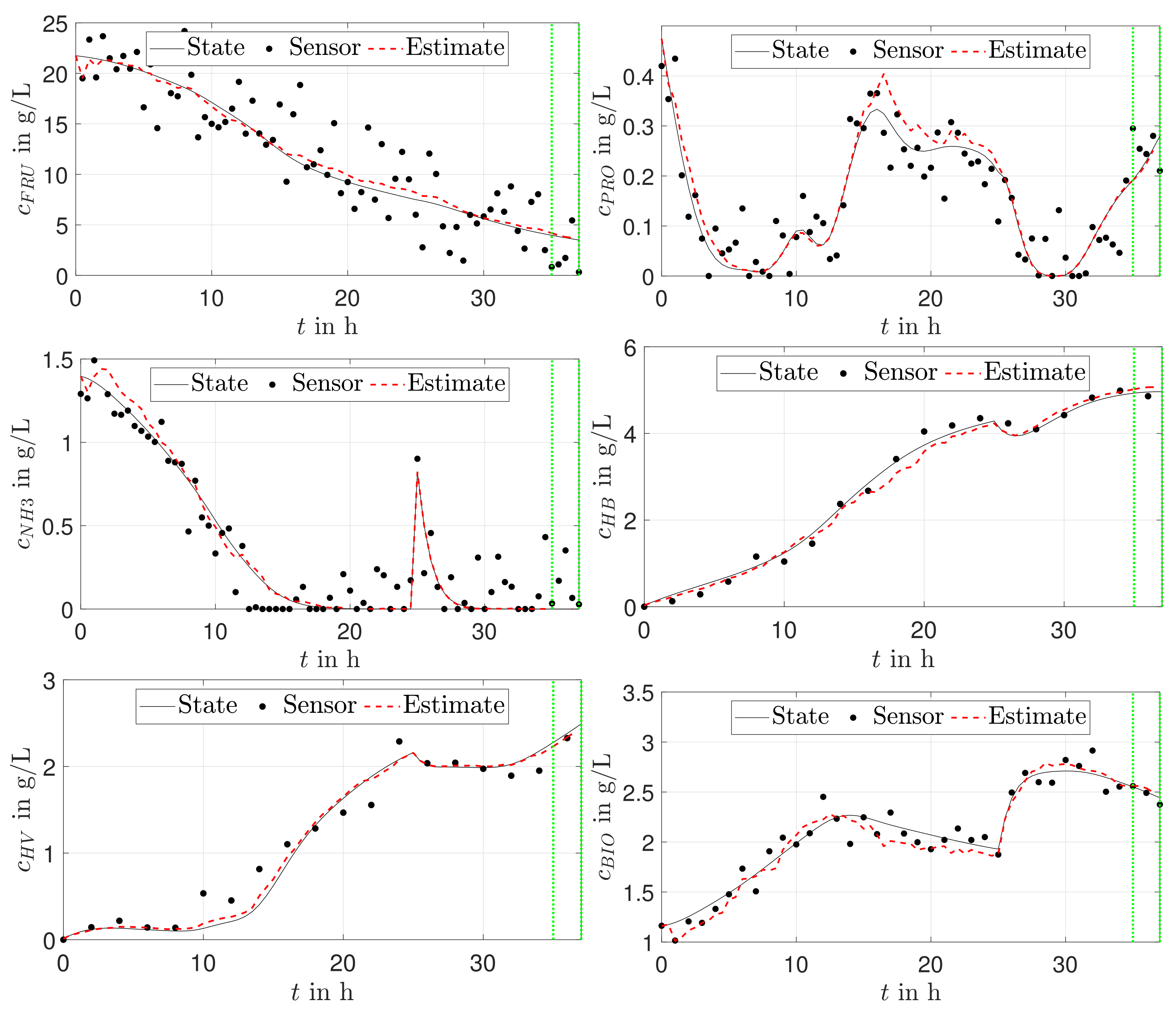
3.2. Microbial PHA Production

Bioplastic is a very promising alternative in comparison to conventional plastic raw material, e.g., polypropylene and polyethylene. Polyhydroxyalkanoates (PHAs) represent a very prominent bio-based and bio-degradable group of bioplastic that can be produced in a wide variety of microorganisms. Beside the well-known representative poly-3-hydroxybutyrate (PHB), the co-polymer poly(3-hydroxybutyrate-co-3-hydroxyvalerate) (PHBV) is more competitive in comparison to PHB because of its higher elongation-to-break values, lower melting points and higher biocompatibility [25]. Because of the high production costs for bioplastics such as PHBV, they have a low market share in the plastics industry.

To make bioplastics even more competitive, model approaches can be used to analyze, optimize and finally control the production in order to reduce the costs. In the following section, our recently developed PHBV production model based on online CO${}_2$ exhaust gas measurements to capture biomass growth is described [23].

3.2.1. Model Formulation

The nonlinear model was presented in [23] and describes the dynamics of a fed-batch process using fructose ($c_{fru}$) and propionic acid ($c_p$) as carbon sources. Furthermore, the dynamics of the nitrogen source $c_n$, residual biomass $c_{res}$, HB-content $c_{hb}$ and HV-content $c_{hv}$ are accounted for. The resulting model therefore comprises a system of six nonlinear ordinary differential equations as reported in the Appendix A. The parameter values and detailed description can be found in the original publication [23].

In contrast to the previous example, the process’ dynamics are assumed to be described completely by the deterministic dynamics. In the following, it is assumed that measurements are based on physical samples. Furthermore, it is assumed that substrates concentrations can be determined within $t_{del,1}$ = 30 min and the measurements are accompanied by medium measurement noise. In contrast, analysis of biomass content takes $t_{del,2}$ = 1 h with assessment of HV and HB content takes $t_{del,3}$ = 2 h with low noise. The approach described previously was adapted accordingly to deal with the situation. In contrast to the original publication, only artificial data is used in this simulation study.

3.2.2. State Estimation

In Figure 4 the simulation results are shown.

It can be seen that the filter is able to smooth out the substrate measurements after a short period of adaption. However, propionate estimates deteriorate between 15 h and 25 h. However, after the ammonium-shot estimation accuracy improves rapidly. This may also give hint for future experiments that additional substrate shots could improve the general reconstruction quality. Furthermore, measurements of HB and HV are accurately reconstructed. Estimation of the non-polymeric biomass shows less smooth behavior in comparison, so the reconstruction of residual biomass is more sensitive to measurement noise.

3.2.3. Simultaneous State and Parameter Estimation

In Figure 5 simulation results are shown for simultaneous estimation of the states and the parameter $c_{p,inh}$. It can be seen that the approach is able to reconstruct the states accurately and also the unknown constant parameter. However, during design it was observed that the performance of the parameter estimation is rather sensitive to the UKF’s tuning parameters, i.e., $\kappa$ and Q, which may require more advanced approaches in future when additional parameters have to estimated simultaneously.

4. Conclusions and Outlook

In this article a UKF-based model-based state estimation concept was presented which is able to incorporate delayed and multirate measurement from different sensor. Performance has been evaluated for two different examples: The first example was an exothermic chemical reactor described by nonlinear dynamic equations. It was shown that states as well as unknown parameters can be reconstructed with sufficient accuracy within and outside the corresponding delay window. To the authors opinion the increased computational effort resulting from the more involved implementation is more than compensated by the improved estimation accuracy. In a second example, the method was applied for state estimation of a microbial biopolymer production process. Here, three different sensor delays and sampling rates were assumed and required the adaption of previously presented method. Compounds with a slow sampling rate could be reconstructed accurately. Furthermore, the approach was adapted to allow for simultaneous reconstruction of an unknown model parameter. The results showed sufficient performance despite being rather sensitive to the UKF’s tuning.

The overall results indicate that the presented method is a promising approach for online state and parameter estimation in (bio-)chemical processes. The UKF implementation is able to accurately reconstruct both from noisy and multirate measurements which are found often in practice due to manifold measurement devices and complex analysis techniques based on physical samples. It thereby represents a valuable tool for advanced automatic control concepts which rely on accurate information on the corresponding process despite limited and delayed measurement information. The authors would also like to emphasize, that the presented concept for multirate data fusion does not involve complex computations such as solution of inverse problems by nonlinear optimization, as found in alternative approaches. Therefore, real-world and real-time realization does not require excessive computational power but could also be accomplished using rather simple platforms.

In the future, focus will be on application of the approach for control of (bio-) chemical processes. Examples include biopolymer production from agricultural and food industrial waste streams [26,27,28] as well as bakers yeast drying [29,30,31]. For more complex cases with multiple unknown parameters, higher nonlinearities or non-Gaussian process noise, performance of the UKF approach may deteriorate. Here, particle filters [6,32] can represent a promising alternative. Furthermore, the outlined approach could be used to extend existing estimators for distributed parameter systems as found in the description of particle formation [33,34,35] and biotechnological processes [36,37,38], to reconstruct the systems states and parameters in presence of measurement delays or multi-rate measurements.

References

1. Ge, Z. Review on data-driven modeling and monitoring for plant-wide industrial processes. Chemom. Intell. Lab. Syst. 2017, 171, 16–25. [Google Scholar] [CrossRef]
2. Ge, Z. Process Data Analytics via Probabilistic Latent Variable Models: A Tutorial Review. Ind. Eng. Chem. Res. 2018, 57, 12646–12661. [Google Scholar] [CrossRef]
3. Mohd Ali, J.; Ha Hoang, N.; Hussain, M.; Dochain, D. Review and classification of recent observers applied in chemical process systems. Comput. Chem. Eng. 2015, 76, 27–41. [Google Scholar] [CrossRef] [Green Version]
4. Haug, A. Bayesian estimation for target tracking, Part I: General concepts. Wiley Interdiscip. Rev. Comput. Stat. 2012, 4, 375–383. [Google Scholar] [CrossRef]
5. Haug, A. Bayesian estimation for target tracking, Part II: The Gaussian sigma-point Kalman filters. Wiley Interdiscip. Rev. Comput. Stat. 2012, 4, 489–497. [Google Scholar] [CrossRef]
6. Haug, A. Bayesian estimation for target tracking, Part III: Monte Carlo filters. Wiley Interdiscip. Rev. Comput. Stat. 2012, 4, 498–512. [Google Scholar] [CrossRef]
7. Khatibisepehr, S.; Huang, B.; Khare, S. Design of inferential sensors in the process industry: A review of Bayesian methods. J. Process. Control 2013, 23, 1575–1596. [Google Scholar] [CrossRef]
8. Patwardhan, S.C.; Narasimhan, S.; Jagadeesan, P.; Gopaluni, B.; Shah, S.L. Nonlinear Bayesian state estimation: A review of recent developments. Control Eng. Pract. 2012, 20, 933–953. [Google Scholar] [CrossRef]
9. Robertson, D.G.; Lee, J.H.; Rawlings, J.B. A moving horizon-based approach for least-squares estimation. AIChE J. 1996, 42, 2209–2224. [Google Scholar] [CrossRef]
10. Rao, C.V.; Rawlings, J.B.; Mayne, D.Q. Constrained state estimation for nonlinear discrete-time systems: Stability and moving horizon approximations. IEEE Trans. Autom. Control 2003, 48, 246–258. [Google Scholar] [CrossRef] [Green Version]
11. Valluru, J.; Patwardhan, S.C.; Biegler, L.T. Development of robust extended Kalman filter and moving window estimator for simultaneous state and parameter/disturbance estimation. J. Process. Control 2018, 69, 158–178. [Google Scholar] [CrossRef]
12. Simon, D. Optimal State Estimation: Kalman, H-Infinity, and Nonlinear Approaches; John Wiley and Sons, Inc.: Hoboken, NJ, USA, 2006. [Google Scholar] [CrossRef]
13. Särkkä, S. Bayesian Filtering and Smoothing; Number 3; Cambridge University Press: New York, NY, USA, 2013. [Google Scholar]
14. Gao, B.; Hu, G.; Gao, S.; Zhong, Y.; Gu, C. Multi-sensor optimal data fusion based on the adaptive fading unscented Kalman filter. Sensors 2018, 18, 488. [Google Scholar] [CrossRef] [PubMed] [Green Version]
15. Kager, J.; Herwig, C.; Stelzer, I.V. State estimation for a penicillin fed-batch process combining particle filtering methods with online and time delayed offline measurements. Chem. Eng. Sci. 2018, 177, 234–244. [Google Scholar] [CrossRef]
16. Tatiraju, S.; Soroush, M.; Ogunnaike, B.A. Multirate nonlinear state estimation with application to a polymerization reactor. AIChE J. 1999, 45, 769–780. [Google Scholar] [CrossRef]
17. Zambare, N.; Soroush, M.; Grady, M.C. Real-time multirate state estimation in a pilot-scale polymerization reactor. AIChE J. 2002, 48, 1022–1033. [Google Scholar] [CrossRef]
18. Lathrop, P.M.; Duan, Z.; Ling, C.; Elabd, Y.A.; Kravaris, C. Modeling and Observer-Based Monitoring of RAFT Homopolymerization Reactions. Processes 2019, 7, 768. [Google Scholar] [CrossRef] [Green Version]
19. Van der Merwe, R. Sigma-Point Kalman Filters for Probablilistic Inference in Dynamic State-Space Models. Ph.D. Thesis, Oregon Health & Science University, Portland, OR, USA, 2004. [Google Scholar]
20. Kalman, R.E. A new approach to linear filtering and prediction problems. J. Basic Eng. 1960, 82, 35–45. [Google Scholar] [CrossRef] [Green Version]
21. Li, T.; Corchado, J.M.; Bajo, J.; Sun, S.; De Paz, J.F. Effectiveness of Bayesian filters: An information fusion perspective. Inf. Sci. 2016, 329, 670–689. [Google Scholar] [CrossRef]
22. Schaffner, J.; Zeitz, M. Entwurf nichtlinearer Beobachter. In Entwurf Nichtlinearer Regelungen; Engell, S., Ed.; Oldenbourg Wissenschaftsverlag: Münich, Germany, 1995. [Google Scholar]
23. Duvigneau, S.; Dürr, R.; Behrens, J.; Kienle, A. Advanced Kinetic Modeling of Bio-co-polymer Poly(3-hydroxybutyrate-co-3-hydroxyvalerate) Production Using Fructose and Propionate as Carbon Sources. Processes 2021, 9, 1260. [Google Scholar] [CrossRef]
24. Higham, D.J. An algorithmic introduction to numerical simulation of stochastic differential equations. SIAM Rev. 2001, 43, 525–546. [Google Scholar] [CrossRef]
25. Strong, P.; Laycock, B.; Mahamud, S.; Jensen, P.; Lant, P.; Tyson, G.; Pratt, S. The Opportunity for High-Performance Biomaterials from Methane. Microorganisms 2016, 4, 11. [Google Scholar] [CrossRef] [PubMed]
26. Dahman, Y.; Ugwu, C.U. Production of green biodegradable plastics of poly (3-hydroxybutyrate) from renewable resources of agricultural residues. Bioprocess Biosyst. Eng. 2014, 37, 1561–1568. [Google Scholar] [CrossRef] [PubMed]
27. Koller, M.; Braunegg, G. Advanced approaches to produce polyhydroxyalkanoate (PHA) biopolyesters in a sustainable and economic fashion. EuroBiotech J. 2018, 2, 89–103. [Google Scholar] [CrossRef] [Green Version]
28. Tsang, Y.F.; Kumar, V.; Samadar, P.; Yang, Y.; Lee, J.; Ok, Y.S.; Song, H.; Kim, K.H.; Kwon, E.E.; Jeon, Y.J. Production of bioplastic through food waste valorization. Environ. Int. 2019, 127, 625–644. [Google Scholar] [CrossRef] [PubMed]
29. Bück, A.; Seidel, C.; Dürr, R.; Neugebauer, C. Robust feedback control of convective drying of particulate solids. J. Process. Control 2018, 69, 86–96. [Google Scholar] [CrossRef]
30. Dürr, R.; Bück, A. Influence of moisture control on activity in continuous fluized bed drying of baker’s yeast pellets. Dry. Technol. 2020, 1–6. [Google Scholar] [CrossRef]
31. Dürr, R.; Seidel, C.; Neugebauer, C.; Bück, A. Self-tuning control of continuous fluidized bed drying of baker’s yeast pellets. Dry. Technol. 2020, 38, 646–654. [Google Scholar] [CrossRef]
32. Dürr, R.; Waldherr, S. A Novel Framework for Parameter and State Estimation of Multicellular Systems Using Gaussian Mixture Approximations. Processes 2018, 6, 187. [Google Scholar] [CrossRef] [Green Version]
33. Bück, A.; Peglow, M.; Tsotsas, E.; Mangold, M.; Kienle, A. Model-based measurement of particle size distributions in layering granulation processes. AIChE J. 2011, 57, 929–941. [Google Scholar] [CrossRef]
34. Mangold, M. Use of a Kalman filter to reconstruct particle size distributions from FBRM measurements. Chem. Eng. Sci. 2012, 70, 99–108. [Google Scholar] [CrossRef]
35. Geyyer, R.; Dürr, R.; Temmel, E.; Li, T.; Lorenz, H.; Palis, S.; Seidel-Morgenstern, A.; Kienle, A. Control of continuous mixed solution mixed product removal crystallization processes. Chem. Eng. Technol. 2017, 40, 1362–1369. [Google Scholar] [CrossRef] [Green Version]
36. Müller, T.; Dürr, R.; Isken, B.; Schulze-Horsel, J.; Reichl, U.; Kienle, A. Distributed modeling of human influenza a virus–host cell interactions during vaccine production. Biotechnol. Bioeng. 2013, 110, 2252–2266. [Google Scholar] [CrossRef] [PubMed]
37. Dürr, R.; Müller, T.; Duvigneau, S.; Kienle, A. An efficient approximate moment method for multi-dimensional population balance models—Application to virus replication in multi-cellular systems. Chem. Eng. Sci. 2017, 160, 321–334. [Google Scholar] [CrossRef] [Green Version]
38. Duvigneau, S.; Dürr, R.; Laske, T.; Bachmann, M.; Dostert, M.; Kienle, A. Model-based approach for predicting the impact of genetic modifications on product yield in biopharmaceutical manufacturing—Application to influenza vaccine production. PLoS Comput. Biol. 2020, 16, 1–22. [Google Scholar] [CrossRef] [PubMed]
Figure 1. State estimation for exothermic reactor before (left) and after (right) slow conversion sensor measurement (black diamond) is available: Estimates of x 1 ( t ) and x 2 ( t ) improve in the delay window (between the green horizontal lines) if measurement of x 1 ( t ) becomes available.
Processes 09 01990 g001
Figure 2. State estimation for exothermic reactor for t = 60 : Accurate reconstruction in face of stochastic process dynamics.
Processes 09 01990 g002
Figure 3. Simultaneous state and parameter estimation for nonlinear exothermic reactor: Results indicate that states and parameters can be reconstructed accurately. Yet, in particular for b ^ 2 and early time points estimates improve significantly if slow sensor measurement is available.
Processes 09 01990 g003
Figure 4. State estimation for microbial PHA production: Accurate reconstruction.
Processes 09 01990 g004
Figure 5. Simultaneous state and parameter estimation for microbial PHA production.
Processes 09 01990 g005