Article

Distributed Secondary Voltage Control for DC Microgrids with Consideration of Asynchronous Sampling

1
School of Electrical Engineering, Southeast University, Nanjing 210096, China
2
Jiangsu Provincial Key Laboratory of Smart Grid Technology and Equipment, Southeast University, Nanjing 210096, China
*
Author to whom correspondence should be addressed.
Processes 2021, 9(11), 1992; https://doi.org/10.3390/pr9111992
Submission received: 20 October 2021 / Revised: 28 October 2021 / Accepted: 31 October 2021 / Published: 8 November 2021
(This article belongs to the Section Process Control and Monitoring)

Abstract

:
This paper studies the distributed secondary control of DC microgrids (MGs) in the case of asynchronous sampling, including both the stability condition and accurate consensus algorithm. The asynchrony means that the update actions of each distributed generation (DG) based on the local information and information received from neighbors are independent of the actions of others at sampled discrete times, which would cause deviation from the accurate convergence and even lead to instability in the worst case. First, a small-signal model of MG installed with secondary voltage control is established to include the individual sampling periods. A stability criterion based on the periodic continuity of sampling instant offset is thus formulated to reveal a stability mapping of multiple sampling. By quantifying the accuracy deviations caused by the asynchrony, an improved ratio consensus strategy is proposed that allows the deviation to be estimated accurately via an auxiliary signal and compensated with respect to the eventual equilibrium to produce an exact solution. Our approach customizes the stability and accuracy for distributed secondary control considering asynchronous sampling in MG, which has been ignored in most existing literature. The effectiveness of the proposed methodology is verified by simulations.

1. Introduction

With the increasing penetration of renewable energy resources, the microgrid (MG) has emerged as a promising concept for integration of distributed generations (DGs), storages and loads within an identifiable electrical boundary [1,2,3]. Typically, an MG can operate while connected to the main grid, and the most appealing advantage of MG is its ability to island itself to form an uninterruptible power supply [4]. With increased DGs, storages and loads being used in power systems, the incumbent power generation paradigm is being developed toward a more DC future because of advantages including simple structure and high efficiency [5,6,7], where an appropriate hierarchical control is indispensable to guarantee reliable and efficient operation of MG systems. To realize spontaneous power sharing without critical communication links, primary control is often implemented using the droop paradigm, which would lead to poor power sharing because of the distinct output impedance and voltage deviations involved.
To overcome these disadvantages of primary control, secondary control schemes ranging from centralized to distributed approaches have been proposed. Centralized control assumes the use of a microgrid centralized controller (MGCC) and a complex communication network that reduces system reliability and increases its sensitivity to single points-of-failure [8,9,10]. Inspired by the multiagent cooperative technology, distributed secondary control, where each DG exchanges information with its immediate neighbors via local networks, was proposed in [11] and has attracted considerable interest in numerous literatures [12,13,14,15,16,17]. In ref. [12], the concept of “virtual voltage drop” was introduced to realize current sharing and voltage restoration in DC MG regardless of the type of resistance. A distributed robust control method has been proposed in [13] to implement secondary control in cases of system uncertainties. In ref. [14], a novel unified distributed control strategy was proposed to realize seamless operation mode transitions. By integrating an event-triggered mechanism, a periodic distributed controller was presented, which allowed the information transmission to be both intermittent and relaxed [15]. In ref. [16], an additional controller for the droop coefficient was introduced to improve the system’s current sharing performance. In ref. [17], through the distributed iterative learning method, the secondary control in MG was realized without accurate knowledge of the system parameters.
Generally, a control cycle consists mainly of information sampling, updating and processing, as well as command transmission and execution [18], which initiates from the information sampling stage. Most of the existing literature on distributed secondary control is based on the assumption that the sampling actions of heterogeneous DGs are triggered in the same time sequence, i.e., using synchronous sampling instants. However, each DG’s update actions based on the local sampled local information and information received from neighboring units are independent of others’ in the sense that each DG is allowed to adjust its dynamics intermittently and dependently, which is inherent behavior in distributed control systems. As such, completely synchronous information exchange is almost unobtainable without the aid of synchronizers, while asynchronous information exchange among DGs can definitely lead to data interleaving and even disorder [19,20], which would then cause persistent convergence deviations from accurate solutions or even system instability. Additionally, the majority of DGs are integrated into an MG via power electronic inverters and because of their negligible inertia, the DGs can respond rapidly to control commands composed of distinctly sampled information; this in turn makes the cooperativity and controllability of distributed control approach more challenging. It should be noted here that the asynchrony of distributed information exchange has been demonstrated in previous research [21,22] that concerned multiple transmission delays; however, these works addressed delay-dependent stability only ignoring consensus accuracy, while the impact of asynchronous sampling on the overall performance is much more sophisticated because of the accumulated time instant offset.
Motivated by the research gap mentioned above, this paper investigates distributed secondary control for MGs taking the impact of asynchronous sampling into consideration. Using a small-signal dynamic model embedded with diverse sampling periods, the sampling margin of DGs is determined. To address the convergence deviation caused by asynchrony, an improved ratio consensus algorithm is proposed based on deviation compensation. The main contributions are listed below.
(1) Given that each DG unit in a distributed control system updates its dynamics independently, the distributed secondary control in MG with regard to asynchronous sampling is first investigated in this paper, including both the stability condition and an accurate consensus algorithm.
(2) A small-signal MG model with distributed secondary control is established using the normalized periodicity of sampling offset among the interactive DGs, which allows for the stability assessment of MG with asynchronous sampling.
(3) The equilibrium deviation caused by the asynchrony of the distributed information exchange among DGs is analyzed quantitatively. Then, an accurate distributed control based on ratio consensus is proposed, where the deviation is estimated and then compensated via an auxiliary state observer timely.
The remainder of this paper is organized as follows. Section 2 reviews MG hierarchical control and formulates the asynchronous sampling concerns; a small-signal model is then proposed, with sampling stability criteria in Section 3. An improved ratio consensus algorithm is proposed in Section 4. Section 5 validates the effectiveness of proposed method by simulations; finally, conclusions are provided in Section 6.

2. MG Hierarchical Control and Problem Formulation

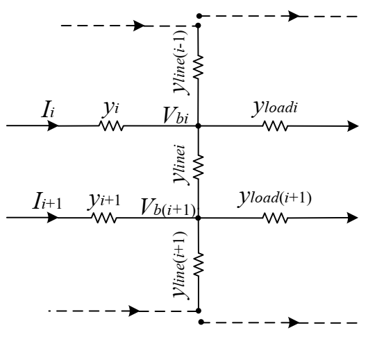
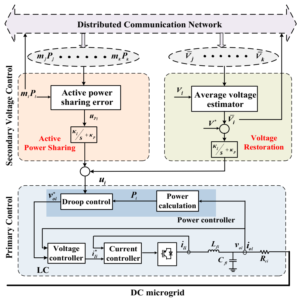
2.1. Primary Control and Distributed Secondary Control

The hierarchical control scheme is widely applied in the MG field using the control structure presented in Figure 1 [23], where each hierarchy is endowed with significant control objective and different timescale. As stated in ref. [24], the bandwidths for the voltage loop and current loop in primary control are 5 kHz and 20 kHz, respectively, while that for secondary control is 30 Hz.
Droop control is adopted as the primary control approach to ensure system stability through voltage and current regulators. The voltage loop is responsible for regulating output voltage to the set-point and a reference for the current loop is also supplied. The error between the actual and expected currents will be calculated and fed into the inner loop to determine the duty cycle to generate PWM for converters [25]. In summary, the complete droop control dynamics can be expressed as [26]:
d θ d t = V n i m i P i V i i r e f = k p v ( V n i m i P i V i ) + k i v θ d ϑ d t = i r e f i i d i = k p i ( i r e f i i ) + k i i ϑ
where Vi and Vni denote the output and nominal voltages, respectively; ii and iref denote the output and reference currents, respectively; kpv and kiv (kpi and kii) are the proportional and integral gains of voltage (current) controller; di represents the duty cycle; mi is droop coefficient; and Pi is active power.
Distributed secondary control is then introduced to realize active power sharing and voltage restoration. Typically, the active powers must be allocated appropriately in inverse proportion to droop coefficients, i.e., m1P1 = m2P2 =…= mnPn [27]. Then, a distributed control scheme that enables elimination of the active power disagreement upi is given as:
u P i = j = 1 , j i n a i j ( m j P j m i P i )
where aij = 1 indicates the information exchanges between the ith and the jth DGs; otherwise, aij = 0. Considering the inherent tradeoff between power sharing and local voltage restoration, the average voltage across the MG is expected to converge to a rated value. An average voltage estimator is then localized in each DG based on the dynamic consensus algorithm [21] to steer its estimated voltage to the practical average voltage:
V ¯ i = V i + k i 3 j = 1 , j i n a i j ( V ¯ j V ¯ i ) d t
where V ¯ i and V ¯ j denote the average voltages from the estimators of the ith and jth DGs, respectively.
Then, the integrated secondary control input is deduced as
u i = ( k p 1 + k i 1 s ) u P i + ( k p 2 + k i 2 s ) ( V n V ¯ i )
where ui is secondary control input; kp1, ki1, kp2 and ki2 denote the proportional and integral gains, respectively. It can be observed from (2) and (3) that the average consensus and the dynamic average consensus as basis of distributed secondary control have an important effect on system performance.

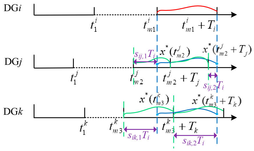
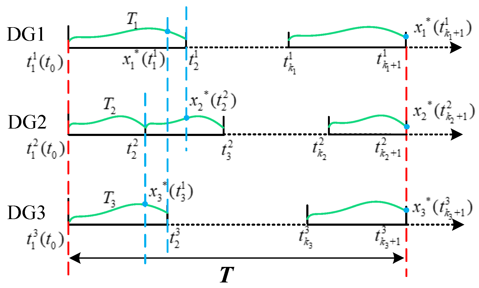
2.2. Problem Formulation of Asynchronous Samplinlg

In the absence of centralized synchronized clock, it is difficult for each DG to update its action at exactly the same time as others; this is inherent in distributed control system. The process of asynchronous information interaction is illustrated in Figure 2, where the secondary control of DGi is triggered at the sampling instant t m 1 i and it receives the most recently sampled information x* from its neighbors, which comes from their latest update timeslots, t m 2 i and t m 3 i , which lag behind t m 1 i with a varying offset sij,mTi at each sampling instant. Therefore, the signal asynchrony and further convergence deviation appear.
Suppose pij is the total number of possible sampling instant offsets during information transmission from the jth DG to ith DG and 1/pij is then denoted as the distribution function of sampling offset corresponding to sij,m for m ∈ [1, pij] (see the explanation in Appendix A). For more practical implementation, a discrete form of the consensus algorithm that considers asynchronous control periods is formulated as [28]:
x i ( k + 1 ) = ( 1 d i ε T i ) x i ( k ) + ε T i j N i [ m = 1 p i j 1 p i j x j ( k s i j , m ) ]
where di denotes the degree of the ith DG, di = ∑jaij; ε represents the interaction strength and Ti denotes the control period. Specifically, pij and sij,m can be formulated as:
p i j = l c m ( T i , T j ) T i , s i j , m = mod ( m T i / T j ) T i
where lcm(x, y) represents the least common multiple of x and y and mod(·) represents its remainder.
For the integrity of time sequences for (5), the discretization period in (6) is reselected to be sbTi, where sb is the largest common divisor of all possible time deviations, i.e., sb = gcd ({sij,m | i, j ∈ [1,n], m ∈ [1, pij]}), where gcd (·) is the largest common divisor. Accordingly, (6) can then be rewritten as:
x i ( k + h ) = ( 1 d i ε T i ) x i ( k ) + ε T i j N i [ m = 1 p i j 1 p i j x j ( k r i j , m ) ]
where h = 1/sb and rij,m = sij,m/sb.
Let x(k + r) = [x1(k + r), x2(k + r), …, xn(k + r)]T and X(k) = [x(k + h − 1), x(k + h − 2), …, x(krmax)]T, where rmax represents the maximum of rij,m. Then, a compact form of (7) yields:
X ( k + h ) = A 1 X ( k )
where A1 is a row stochastic matrix that is directly related to the individual sampling periods (listed in the Appendix A); 1 is an eigenvalue of A1 along the corresponding right eigenvector [1, 1, …, 1]T, which implies that all states converge to a constant value. The eigenvalues of A1 are defined as λn ≤ … ≤ λ2λ1, with ui and vi as the left and right eigenvectors that correspond to λi, respectively. Therefore, the initial state X(0) can be expressed using the eigenbasis of A1 as X(0) = i = 1 n ( u i X ( 0 ) ) v i , and then
lim k X ( k ) = lim k i = 1 n λ i k h ( u i X ( 0 ) ) v i
Considering the sufficient and necessary condition to reach consensus to be maxi ≥ 2|λi| < 1, it can be inferred that limkX(k) = (u1X(0))v1 with v1 = [1, 1, …, 1]T. Consequently, the final convergence value of x can be expressed as:
c x = u 1 X ( 0 )
where u1 is the left eigenvector of A1 corresponding to the eigenvalue 1. As shown in (10), in addition to the control parameters, the distributed consensus equilibrium is dependent on the individual sampling instants, corresponding to the sampling time offset, which is the main focus of this paper.
For the dynamic consensus, we suppose that all the dynamic states have converged to cx’ at t = t0, and the instant variation of the dynamic state at t = t0 is then modeled as the step function Δzi. The accurate average value can then be expressed as u2Δz, where u2 represents the left eigenvector of L and L = DΛ with D = diag(di) and Λ = [aij]. The deviation of the consensus equilibrium from its accurate counterpart can be calculated as:
Δ c x = ( u u 2 ) Δ z
where u′ = [ k = 0 h u 1 ( n k + 1 ) , …, k = 0 h u 1 ( n k + n ) ]T and Δz = [Δz1, Δz2, …, Δzn]T. Therefore, the convergence deviation of dynamic consensus is decided not only by the factor in average consensus (10) but also by the variations of the dynamic states, which makes achieving convergence accuracy more challenging.

3. Stability Analysis in the Asynchronous Sampling Period Case

In this section, a small-signal dynamic model of an islanded MG is established. It allows for the determination of stability region for the individual sampling periods of DGs.

3.1. Small-Signal Modeling

An MG model typically comprises three specific components: the inverters, the network and the loads. Given the fairly rapid response of double-loop controller when compared with that of power loop, we consider the dynamics of the power control loop only and neglect those of the double-loop [22]:
V i = V n i m i P i + u i
where Pi can be measured using a low-pass filter:
P ˙ i = ω f P i + ω f V i I i
where ωf denotes the filter cutoff frequency and Ii denotes the output current of the ith DG.
It is assumed that n DGs are connected to the load network and the network structure is then as shown in Figure 3.
Thus, the output current can be given as:
I = Y ( V V b )
where I = [I1, I2, …, In]T, V = [V1, V2, …, Vn]T, and Vb = [Vb1, Vb2, …, Vbn]T, with Vbi denoting the voltage of the ith bus; and Y = diag(yi), where yi is the output admittance of the ith DG.
According to the node voltage equation of the network, the ith bus voltage can be determined using:
y s i V b i = y l i n e ( i 1 ) V b ( i 1 ) + y l i n e i V b ( i + 1 ) + y i V i
where ysi = ylinei + yline(i − 1) + yi + yloadi with ylinei and yloadi representing the line and load admittances, respectively.
Combining (14) with (15), the output current and voltage can be arranged in a compact form:
I = Y V
where Y′ = Y(1 − Ys−1Y) and Ys is
Y s = y s 1 y l i n e 1 0 0 y l i n e 1 y s 2 y l i n e 2 0 0 y l i n e ( n 1 ) y s ( n 1 ) y l i n e n 0 0 y l i n e n y s n
Using (3), (4), (12), (13) and (16), we can then obtain
Δ V ˙ i = m i Δ P ˙ i + Δ u ˙ i
Δ P ˙ i = ω f Δ P i + ω f ( I i Δ V i + j = 1 n V i y i j Δ V j )
Δ u ˙ i = k p 1 j = 1 , j i n a i j ( m j Δ P ˙ j m i Δ P ˙ i ) + k i 1 j = 1 , j i n a i j ( m j Δ P j m i Δ P i ) k p 2 Δ V ¯ ˙ i k i 2 Δ V ¯ i
Δ V ¯ ˙ i = Δ V ˙ i + k i 3 j = 1 , j i n a i j ( V ¯ j V ¯ i )
By consolidating (17)–(20), the complete small-signal model of system can then be deduced to be:
Δ x ˙ = A 2 Δ x
where Δ x = [ Δ P 1 ,   ,   Δ P n ,   Δ V 1 , , Δ V n ,   Δ V ¯ 1 , , Δ V ¯ n , ] T and A2 is the coefficient matrix listed in the Appendix A.
Consideration of the significant distinction between the control periods of the primary and secondary layers shows that they would be implemented at their discrete times separately, and the primary control periods of DGs are supposed to be the same. The incremental forms of the droop control and power measurement equations can then be expressed as:
Δ V i ( n + 1 ) Δ V i ( n ) = m i Δ P i ( n ) m i Δ P i ( n + 1 ) + Δ u i ( n + 1 ) Δ u i ( n )
Δ P i ( n + 1 ) Δ P i ( n ) = ω f T s Δ P i ( n ) + ω f T s [ I i Δ V i ( n ) + j = 1 n V i y i j Δ V j ( n ) ]
where Ts denotes the primary control period.
Analogously, the incremental model for secondary control with consideration of the asynchrony can be formulated as:
Δ u i ( n + 1 ) Δ u i ( n ) = k p 1 j = 1 , j i n a i j [ m j ( Δ P j ( n + 1 ) Δ P j ( n ) ) m i ( Δ P i ( n + 1 ) Δ P i ( n ) ) ] + k i 1 T i j = 1 , j i n a i j [ m j Δ P j ( n ) m i Δ P i ( n ) ] + k p 2 [ Δ V ¯ i ( n ) Δ V ¯ i ( n + 1 ) ] k i 2 T i Δ V ¯ i ( n )
Δ V ¯ i ( n + 1 ) Δ V ¯ i ( n ) = Δ V i ( n + 1 ) Δ V i ( n ) + k i 3 T i j = 1 , j i n a i j [ Δ V ¯ j ( n ) Δ V ¯ i ( n ) ]

3.2. Asynchronous Sampling-Dependent Stability Analysis

As demonstrated in Figure 4, supposing that the initial instant of all DGs is uniform at t = t0 and letting T be the least common multiple of all the DG control periods, i.e., T = lcm (T1, T2, …, Tn), the staggered information interaction process continues except for the instant set t = t0 + kT (k = 1, 2, …) when the sampling information in MG is synchronous because of the global timeslot. Therefore, we perform the modeling and analysis within T, which is regarded as a normalized cycle period.
As stated previously, the primary and secondary control layers are operated with different control periods. The primary control instants of individual DGs within the cycle period T are represented by t 1 k , t 2 k , …, t k n , where n = T/Ts, and the update process of the measured powers and voltages at the primary control instant t k l can then be expressed based on (22) and (23):
Δ x ¯ ( t k l + 1 ) = W 1 Δ x ¯ ( t k l ) + H 1 [ Δ u ( t k l + 1 ) Δ u ( t k l ) ]
where Δ x ¯ = [ΔP1, ΔP2, …, ΔPn, ΔV1, ΔV2, …, ΔVn]T; W1 and H1 are the coefficient matrices presented in the Appendix A.
Here, we consider two cases: (1) if secondary control is not activated at t = t l + 1 k , then Δu( t l + 1 k ) − Δu( t 1 k ) = 0; (2) if secondary control is triggered at t = t l + 1 k , then the related variables of the ith DG can be updated as:
Δ u i ( t k l + 1 ) Δ u i ( t k l ) = W i 2 Δ x ¯ ( t k l + 1 ) + W i 3 Δ x ¯ ( t ˜ k ) + G i 1 Δ V ¯ ( t k l + 1 ) + G i 2 Δ V ¯ ( t ˜ k )
Δ V ¯ i ( t k l + 1 ) = W i 4 [ Δ x ¯ ( t k l + 1 ) Δ x ¯ ( t ˜ k ) ] + G i 3 Δ V ¯ i ( t ˜ k )
where x ( t ˜ k ) represents the state from the last secondary control instant that was recorded; Wi2, Wi3, Wi4, Gi1, Gi2, and Gi3 are the coefficient matrices presented in the Appendix A.
By performing n iterations based on the process described above, the discrete small-signal model of MG system within the cycle period T can be arranged as:
Δ x ( t k l + n ) = D 1 Δ x ( t k l )
where D1 is the coefficient matrix shown in the Appendix A.
The eigenvalues of D1 are denoted by λn ≤ … ≤ λ2λ1, and then the asynchronous MG system is stable if and only if all the characteristic roots lie within the unit circle, i.e., max|λi| ≤ 1.

4. Improved Ratio Consensus Algorithm

As shown in Section 2, the average consensus and dynamic consensus are two important aspects of MG secondary control, where the former is a special case of the latter based on the supposition that the local dynamic state disappears. Therefore, for the convenience of analysis, the accuracy improvement for dynamic average consensus is formulated later, and the average consensus can be dealt with in the similar way.

4.1. Ratio Consensus Algorithm

To address the exact observed average equilibrium of distributed control in the presence of communication delays, the ratio consensus algorithm was proposed in [29] as follows:
x ˙ i ( t ) = z ˙ i ( t ) + ε j i a i j [ x j ( t τ ) x i ( t ) ]
y ˙ i ( t ) = ε j i a i j [ y j ( t τ ) y i ( t ) ]
p i ( t ) = x i ( t ) y i ( t )
where zi is the actual dynamic state of ith agent, whose average is being tracked; xi and xj are the average values from the ith and jth observers; yi and pi are state variable and local average observation, respectively and τ is the transmission delay.
The ratio consensus algorithm consists of two parts (30) and (31), of which the simultaneous convergence indicate the consensus of entire protocol. As stated in ref. [30], the observer of the scheme can accurately track the average dynamic states (i.e., xi = N   i = 1 zi/N) only when τ ¯ remains unchanged, otherwise it would lead to convergence error from the exact solution. In contrast to the unchanged τ ¯ , the asynchronous sampling case considered in this paper is notoriously complex because the probability distribution of timeslot for information exchange is time-varying during the sampling procedure, which poses challenge to the ratio consensus algorithm in accurate average.

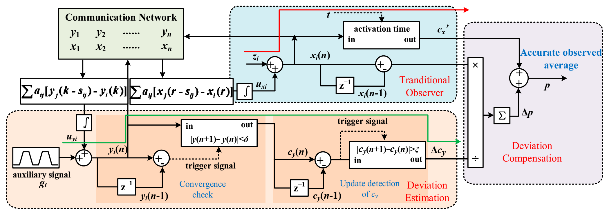
4.2. Improved Consensus Algorithm

In this section, an improved algorithm is proposed to track the accurate consensus equilibrium of MG system in case of asynchronous sampling of DGs. The discrete form of this distributed average estimator is formulated as follows:
x i ( n + 1 ) = z i ( n + 1 ) + ε T i r = 1 n j i a i j [ x j ( r s i j ) x i ( r ) ]
y i ( n + 1 ) = g i ( n + 1 ) + ε T i r = 1 n j i a i j [ y j ( r s i j ) y i ( r ) ]
p ( n + 1 ) = p ( n ) + x ( n + 1 ) x ( n ) Δ c y ( n )
where xi and yi represent the estimated average values of z = [z1, z2, …, zn] and g = [g1, g2, …, gn], respectively; sij denotes the sampling time offset between the ith DG and jth DG, which is time-varying; gi is a predefined slope signal localized in each DG:
g i = f s q u a r e ( t ) min ( k 2 t T g , 1 ) + 3 2 1 2 f s q u a r e ( t )
f s q u a r e ( t ) = 4 π m = 1 sin ( ( 2 m 1 ) t T g ) / ( 2 m 1 )
where fsquare(t) is a square function with variation range [−1, 1]; k is the slope coefficient corresponding to variation dynamics of z; [·] represents the rounding function; Tg is the designed period of gi. It can be observed from (36) and (37) that gi varies with k every Tg and |gmaxgmin| = 1. Δcy = |cycy′|, with cy and cy′ are the estimated average of gi with respect to gmax and gmin, respectively.
The control diagram of the proposed consensus scheme consists of three parts, the traditional dynamic consensus, deviation estimation and compensation as presented in Figure 5. Because of asynchronous information exchange, xi deviates from the accurate average value using traditional observer and the relevant deviation depends on the distribution of sampling instant offset based on Section 2, which is difficult to obtain. It is obvious that zi and gi in each DG can be updated using the uniform control period; hence they share the same time offset distribution. Similar to the time delay case in ref. [27], we denote the deviation factor (DF) here as the ratio of estimated average variation of observer and actual average variation to indicate the impact of asynchronous sampling on consensus accuracy. For the definition of (36), it is easy to calculate DF of gi as
D F = 1 1 + ε s ¯ = | Δ c y | | Δ g | = Δ c y
where s ¯ represents the mean of the sampling time offset; Δg is the actual average variation, |Δg| = |gmaxgmin| = 1 here. Δcy updated every time when gi reaches its maximum or minimum value and is observed locally so DF is accessible for each DG.
Alternatively, the observed average variation of dynamic state zi can be expressed as:
x ( n + 1 ) x ( n ) = 1 1 + ε s ¯ u 2 Δ z
where u2Δz denotes the actual variation of average states.
Considering that zi under track holds the same sampling time offset s ¯ as gi, they also have the same DF. Therefore, the actual variation can thus be obtained without the measurement of time offset even in face of a varying sampling offset during state exchange. Based on (38) and (39), it yields,
u 2 Δ z = x ( n + 1 ) x ( n ) Δ c y
Then, the accurate average states can be observed using
u 2 z = c x + u 2 Δ z
where cx′ is the consensus value obtained from the traditional dynamic observer as shown in Figure 5. Combining (40) and (41), the improved dynamic observer can be formulated in (35) with the deviation estimated and compensated step by step, to arrive at an exact consensus solution eventually.
As discussed above, the deviation estimation is of most significance for the proposed accurate consensus algorithm. To guarantee properly determination of Δcy every step, a convergence check and an update detection module are applied as shown in Figure 5. The judgment condition for the convergence check can be expressed as |y(n + 1) − y(n)| < δ, where δ is a preset upper error bound. When the condition above is satisfied, it can be deduced that y converges to a new equilibrium, which then become the updated output; otherwise, the previous value will hold, so cy is available if a step variation in gi. Additionally, |cy(n + 1) − cy(n)| is measured to detect the update action of cy, where |cy(n + 1) − cy(n)| > ξ indicates that cy has updated to a new value with a threshold ξ and Δcy can then be obtained as |cy(n + 1) − cy(n)|. In order to avoid the misjudgment of Δcy update, it should be satisfied that ξ > δ. Ultimately, a precise average estimation can be realized due to the accessible compensation. As average consensus is a special case of dynamic consensus, the proposed algorithm can also be utilized for accurate average convergence, which is demonstrated from power sharing.

5. Simulation Results

Case studies are performed to investigate the secondary control performance under asynchronous sampling conditions using a test DC microgrid shown in Figure 6, where the system and control parameters are listed in Table 1 and the desired power sharing ratio among the three DG units is 1:1:1. For simplification, the test system consisting of three DGs is considered, whereas the method proposed in this paper is also applicable to systems with larger scales. Moreover, note that this paper focuses on the effect of distinct sampling, so a cycle network is adopted which can be modified to other connected forms. Simulation results using MATLAB/Simulink are utilized to verify the effectiveness of the proposed criterion.

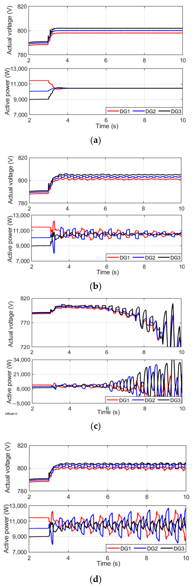
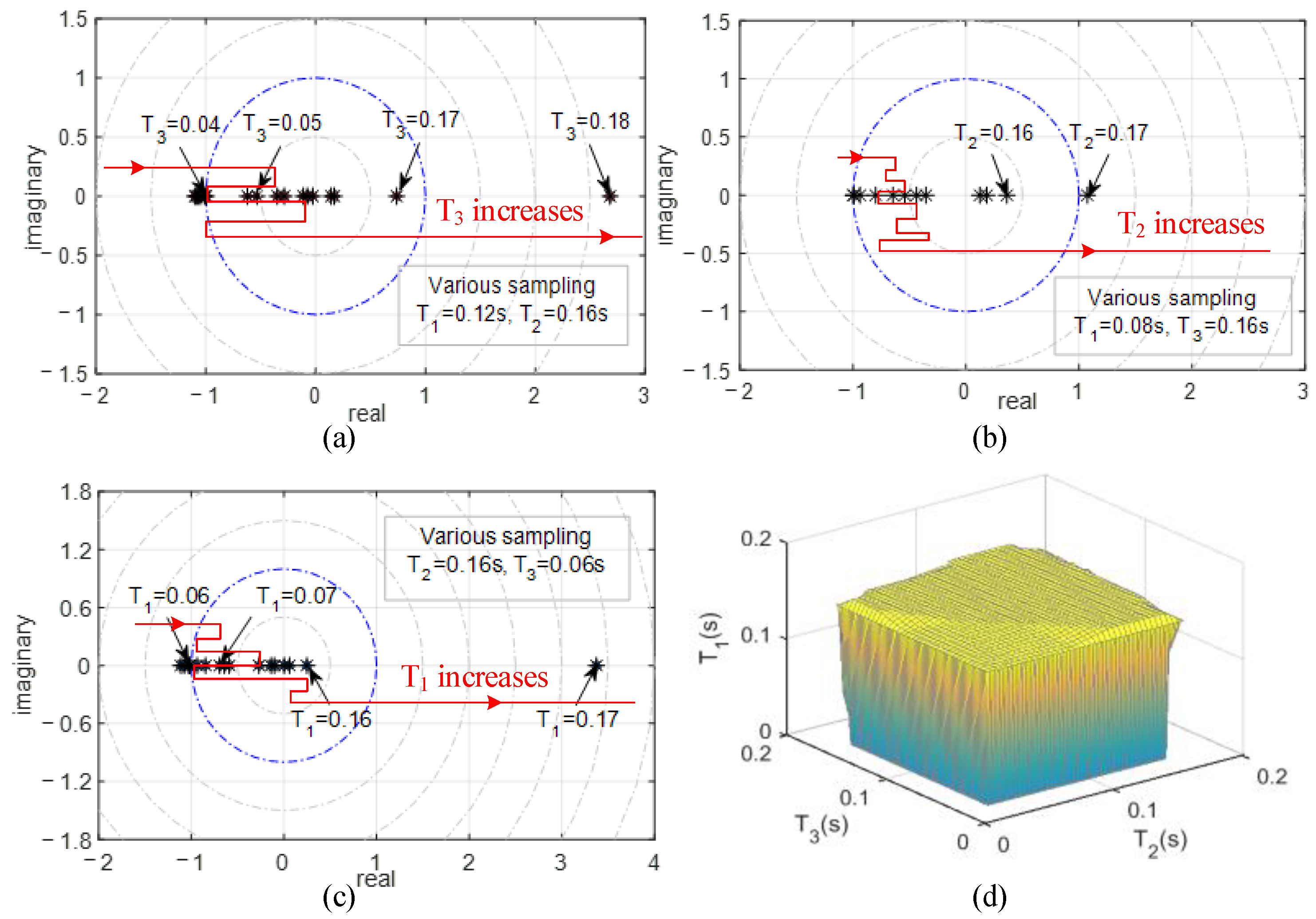
5.1. Stability Analysis

(1) Theoretical stability region of control periods: The control period of each DG is assumed to be independent of others and the sampling-dependent stability region is calculated using the method proposed in Section 3. Figure 7a–c shows the dominant root loci of state matrix D1 in (29), revealing the critical sampling periods which occupies the unit cycle. It can be found that generally as the control period increases, the eigenvalues move from the inside of unit circle to the outside, which indicates a less stable system. Another significant phenomenon is that the system could also become unstable with a great disagreement among the control periods. It can be observed that when T1 = 0.12 s and T2 = 0.16 s, the MG system becomes unstable if T3 ≤ 0.04 s due to the notable sampling inconsistence. This is in contrast to the widely held opinion that the smaller control period is, the more stable system is and is crucial for the design of control period. Similarly, the stability mapping with regard to multiple independent control periods are yielded and the results are depicted in Figure 7d.
(2) Simulation verification of stability region: To validate the theoretically calculated stability region, simulation studies are performed with T1 = 0.12 s, T2 = 0.16 s and different T3. The MG is initially controlled by droop control and secondary voltage control is activated at t = 3 s. The effectiveness of secondary control is verified with the consistent control period T1 = T2 = T3 = 0.1 s as shown in Figure 8a, where the voltage deviates and proper power sharing fails initially and after launching secondary control, the voltages restore and power is accurately apportioned. Figure 8b–d display the corresponding responses for asynchronous cases. For T3 = 0.07 s, the simulation results in Figure 8b experience violent but decaying oscillations. With an increased control period T3 = 0.18 s, the MG becomes unstable due to the growing oscillations. Then, the T3 stability region lies within [0.07 s, 0.18 s] for T1 = 0.12 s and T2 = 0.16 s, which coincides with the theoretically calculated range [0.05 s, 0.017 s] (see Figure 7a). However, for a relatively small value T3 = 0.04 s, the system tends to be unstable as shown in Figure 8d because of the notable sampling disagreement. Therefore, we confirm the validity of the proposed stability analysis criterion.

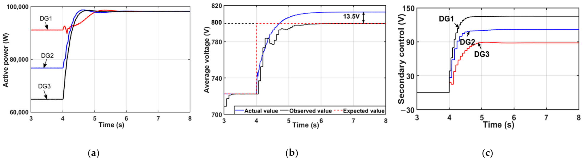
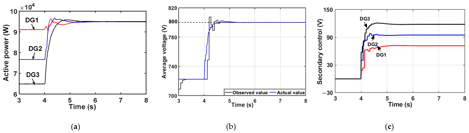
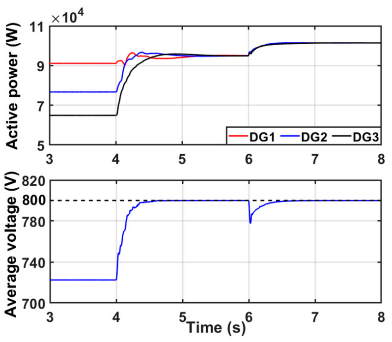
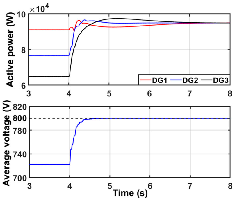
5.2. Accuracy Analysis

(1) Theoretical Analysis of Consensus Deviation. Case studies are developed with the sampling set (T1 = 0.07 s, T2 = 0.08 s and T3 = 0.05 s) to verify the accurate consensus convergence of the proposed algorithm. In this case, the average sampling time offset s ¯ i j during information interactions between any two DGs can be calculated to be s ¯ 12 = 0.035 s, s ¯ 13 = 0.02 s, s ¯ 21 = 0.03 s, s ¯ 23 = 0.02 s, s ¯ 31 = 0.03 s, and s ¯ 32 = 0.035 s in this case. Provided that the threshold of average sampling time offset estimation is 1/5 s ¯ min , it can be derived that N12T1 = 0.484, N13T1 = 0.245, N21T2 = 0.46, N23T2 = 0.28, N31T3 = 0.2875, and N32T3 = 0.34.
(2) Simulation verification for accurate consensus. To illustrate the superiority of proposed consensus algorithm, a comparison with conventional consensus scheme is performed with the same operation. Initially, the system operates under the individual effect of droop control, where the average voltage is remarkably lower than the nominal value and the active power sharing is inappropriate among DGs. After t = 4 s, the secondary control launches and the states of the system tend to adjust to the ideal operating equilibrium. In the traditional dynamic consensus protocol as shown in Figure 9, when the observed average voltage value is regulated to the reference 800 V, an approximate deviation of 13.5 V appears in the estimated average voltage because of the asynchronous sampled information among DGs. Further, we can observe the voltage variation on the occasion of activation of secondary control as Δz = [81 V, 90 V, 102 V]T via simulation responses, and then the theoretical equilibrium deviation is calculated to be Δcx = 19.16 V using the method proposed in Section 2, which is roughly identical to the actual value 13.5 V. As shown in Figure 10, the observed average voltage of proposed consensus algorithm can exactly track the actual average voltage due to the real-time deviation estimation and compensation so that the accurate secondary control is maintained. Moreover, the total output power of the conventional method in Figure 9a is nearly 10 kW higher than that in Figure 10a because of the convergence error. Therefore, the accuracy and effectiveness of the proposed distributed secondary control is verified despite asynchronous sampling instants among individual DGs.
To further demonstrate the effectiveness of the proposed strategy in different cases, the cases of load variation and topology switch are developed, with their simulation results displayed in Figure 11 and Figure 12 respectively. In the first case, an additional load (30 Ω) is connected to the voltage bus Vbus2 at t = 6 s. As can be visualized from Figure 11, the active power of each DG increases and the average voltage decreases at t = 6 s, whereas the average voltage can still restore to the nominal value accurately and the active power would be stable at a new operation equilibrium after a transient process with the assistance of the proposed control strategy.
Further, the topology switch is considered in the second case where the communication link between DG1 and DG3 in the topology is set to be disconnected at t = 4.5 s. As is shown in Figure 12, the convergence rate would become slow due to the reduction in the number of communication links, whereas accurate power sharing and voltage regulation can still be achieved ultimately using the proposed strategy.

5.3. Discussion of the results

According to the simulation results, it can be deduced that:
(1)
The simulation results accord well with the theoretical analysis, which verifies the effectiveness of the proposed analytical method.
(2)
The increase of one individual control period would lead to system instability.
(3)
The enlargement of the disagreement between control periods of various DGs can also cause system instability.
(4)
The asynchronization between control periods would give rise to steady-state deviation when adopting the conventional consensus control, whereas the deviation can be effectively eliminated using the improved ratio consensus algorithm proposed in this paper.
(5)
The proposed algorithm would be effective regardless of load variation or topology switch.

6. Conclusions

In this paper, the stability and convergence accuracy of the distributed secondary control of DC microgrids in the case of asynchronous sampling have been investigated. The stability condition for the sampling periods of DGs is presented based on the periodicity of sampling time offset. Considering the convergence deviation caused by information asynchrony, an accurate distributed control algorithm based on ratio consensus is proposed, where an accurate solution can be achieved by real-time estimation and compensation of deviations. Through simulation testing, the following conclusions can be drawn:
  • The system could come to be unstable when any individual control period becomes larger.
  • Expansion of asynchronous degree can also lead to system instability.
  • Steady-state deviation would occur in case of asynchronous control periods when adopting the conventional consensus control, whereas the deviation can be effectively eliminated using the proposed control method.

Author Contributions

Methodology, G.L.; software, Y.H.; writing—original draft preparation, Y.H.; writing—review and editing, S.L.; supervision, G.L. All authors have read and agreed to the published version of the manuscript.

Funding

This work was supported in part by the National Science Foundation of China under Grant 52007031, the National Science Foundation of Jiangsu Province under Grant BK20200404, the “Zhishan” Yong Scholars Programs of Southeast University and the Project Funding for Jiangsu Provincial Key Laboratory of Smart Grid Technology and Equipment, Southeast University.

Institutional Review Board Statement

Not applicable.

Informed Consent Statement

Not applicable.

Conflicts of Interest

The authors declare no conflict of interest.

Appendix A

Statement: 1/pij is the probability that the time deviation is equal to sij,m for any m ∈ [1, pij].
Explanation: Assume T = lcm(Ti,Tj) = pijTi and there exists a time deviation value s that occurs more than once within period T.
According to the hypothesis, there must be integers m1, m2 ∈ [1, pij], which satisfy:
mod ( m 1 T i T j ) = mod ( m 2 T i T j )
Thereby, there are positive integers k1, k2 meet the equation:
m 1 T i k 1 T j = m 2 T i k 2 T j
Rearranging the equation, it can be obtained that:
( m 1 m 2 ) T i = ( k 1 k 2 ) T j = T
i.e., T′ is the common multiple of Ti and Tj. Meanwhile, given that T is the least common multiple of Ti and Tj, it can be inferred that T′ = cT, and thus m1m2 = cpij, where c is a positive integer. Whereas the result that m1 = m2 + cpij contradicts the assumption that m1, m2 ∈ [1, pij], implying the invalidation of the hypothesis. Therefore, each time deviation value can only occur once within period T. Further, consider the secondary control of the ith and jth DG is synchronous at t0, they will synchronize again at t0 + T. Thus, it can be inferred that the change of the time deviation of information transmission between the ith and jth DG is periodic with respect to T.
Synthesize the above analysis, the conclusion can be drawn that it is equiprobable for the time deviation to be equal to any possible value sij,m during a certain information transmission from the jth DG to the ith DG.
A 1 = A 11 I n r max × n r max 0 n r max × n h n ( h + r max ) × n ( h + r max )
where A 11 = C n × n ( h + r max ) C n × n ( h + r max ) n h × n ( h + r max ) and C = 0 n × n ( h 1 ) H n × n f n × n r max n × n ( h + r max ) with H n × n = 1 ε T 1 ε T 1 p 12 ε T 1 p 1 n ε T 2 p 21 1 ε T 2 ε T 2 p 2 n ε T n p n 1 ε T n p n 2 1 ε T n n × n .
f ( i , n ( m 1 ) + j ) = ε T i p i j i f k [ 1 , p i j ] , r i j , k = m 0 o t h e r w i s e
R 1 = I n × n 0 n × n 0 n × n M + k p 1 L M I n × n k p 2 I n × n 0 n × n I n × n I n × n
B = S 1   n × n ω f T s ( I + V Y ) 0 n × n k i 1 L M 0 n × n k i 2 I n × n 0 n × n 0 n × n k 3 L
R 2 = I n × n 0 n × n M n × n I n × n
B 1 = S 2   n × n ω f T s ( I + V Y ) M n × n I n × n
C 1 = 0 n × n 0 n × n 0 n × n I n × n
I n × n = 1 0 0 0 1 0 0 0 1 n × n
S 1   n × n = ω f 0 0 0 ω f 0 0 0 ω f n × n
S 2   n × n = 1 ω f T s 0 0 0 1 ω f T s 0 0 0 1 ω f T s n × n
W i 2 = k p 1 M i 1 0 1 × n 1 × 2 n , W i 3 = W i 2 + k i 1 T i M i 1 0 1 × n 1 × 2 n , G i 1 = k p 2 e i , G i 2 = G i 1 k i 2 T i e i , W i 4 = 0 1 × n e i 1 × 2 n , G i 3 = e i + k i 3 T i L i 1 with e i = 0 0 1 i t h 0 0 1 × n , M i 1 = m 1 m i 1 d i m i m i + 1 m n 1 × n and L i 1 = 1 1 d i 1 1 1 × n .
The acquisition of D1 can be implemented as follows: for l ∈ [1,n], suppose ni control instants are included in a secondary control period of the ith DG, i.e., ni = Ti/Ts; D 1 ( 0 ) = I 3 n × 3 n if t k l + 1 is not a secondary control instant, i.e., mod(l/ni) ≠ 0 for any i
D 1 ( l ) = W ¯ 1 D 1 ( l 1 )
where W ¯ 1 = W 1 0 2 n × n 0 n × 2 n I n × n 3 n × 3 n , if t k l + 1 is a secondary control instant of the ith DG, i.e., mod(l/ni) = 0.
D 1 ( l ) = R ¯ 1 ( W ¯ D 1 ( l 1 ) + H ¯ V i )
R ¯ = I 2 n × 2 n H 1 W 2 H 1 G 1 W 4 I 2 n × 2 n 3 n × 3 n
W ¯ = W 1 0 2 n × n 0 n × 2 n 0 n × n 3 n × 3 n
H ¯ = H 1 W 3 H 1 G 2 W 4 G 3 3 n × 3 n with W 2 = e i T W i 2 , W 3 = e i T W i 3 , G 1 = e i T G i 1 , G 2 = e i T G i 2 , W 4 = e i T W i 4 , G 3 = e i T G i 3 .
Then Vi will be updated as V i = D 1 ( l ) .
After n iterations, it can be obtained that D 1 = D 1 ( n ) .

References

  1. Yu, K.; Ai, Q.; Wang, S.; Ni, J.; Lv, T. Analysis and optimization of droop controller for microgrid system based on small-signal dynamic model. IEEE Trans. Smart Grid 2016, 7, 695–705. [Google Scholar] [CrossRef]
  2. Lou, G.; Gu, W.; Xu, Y.; Jin, W.; Du, X. Stability robustness for secondary voltage control in autonomous microgrids with consideration of communication delays. IEEE Trans. Power Syst. 2018, 33, 4164–4178. [Google Scholar] [CrossRef]
  3. Liu, S.; Wang, X.; Liu, P.X. Impact of communication delays on secondary frequency control in an islanded microgrid. IEEE Trans. Ind. Electron. 2015, 62, 2021–2031. [Google Scholar] [CrossRef]
  4. He, J.; Li, Y.W. Analysis, design, and implementation of virtual impedance for power electronics interfaced distributed generation. IEEE Trans. Ind. Appl. 2011, 47, 2525–2538. [Google Scholar] [CrossRef]
  5. Li, Z.; Shahidehpour, M. Small-signal modeling and stability analysis of hybrid AC/DC microgrids. IEEE Trans. Smart Grid 2019, 10, 2080–2095. [Google Scholar] [CrossRef]
  6. Dong, M.; Li, L.; Nie, Y.; Song, D.; Yang, J. Stability analysis of a novel distributed secondary control considering communication delay in DC microgrids. IEEE Trans. Smart Grid 2019, 10, 6690–6700. [Google Scholar] [CrossRef]
  7. Dou, C.; Yue, D.; Guerrero, J.M.; Xie, X.; Hu, S. Multiagent system-based distributed coordinated control for radial DC microgrid considering transmission time delays. IEEE Trans. Smart Grid 2017, 8, 2370–2381. [Google Scholar] [CrossRef] [Green Version]
  8. de Nadai Nascimento, B.; Zambroni de Souza, A.C.; Marujo, D.; Sarmiento, J.E.; Alvez, C.A.; Portelinha, F.M., Jr.; de Carvalho Costa, J.G. Centralised secondary control for islanded microgrids. IET Renew. Power Gener. 2020, 14, 1502–1511. [Google Scholar] [CrossRef]
  9. Qian, T.; Liu, Y.; Zhang, W.; Tang, W.; Shahidehpour, M. Event-triggered updating method in centralized and distributed secondary controls for islanded microgrid restoration. IEEE Trans. Smart Grid 2020, 11, 1387–1395. [Google Scholar] [CrossRef]
  10. Guo, F.; Xu, Q.; Wen, C.; Wang, L.; Wang, P. Distributed secondary control for power allocation and voltage restoration in islanded DC microgrids. IEEE Trans. Sustain. Energy 2018, 9, 1857–1869. [Google Scholar] [CrossRef]
  11. Nasirian, V.; Moayedi, S.; Davoudi, A.; Lewis, F.L. Distributed cooperative control of DC microgrids. IEEE Trans. Power Electron. 2015, 30, 2288–2303. [Google Scholar] [CrossRef]
  12. Xing, L.; Mishra, Y.; Guo, F.; Lin, P.; Yang, Y.; Ledwich, G.; Tian, Y. Distributed secondary control for current sharing and voltage restoration in DC microgrid. IEEE Trans. Smart Grid 2020, 11, 2487–2497. [Google Scholar] [CrossRef]
  13. Baranwal, M.; Askarian, A.; Salapaka, S.; Salapaka, M. A distributed architecture for robust and optimal control of DC microgrids. IEEE Trans. Ind. Electron. 2019, 66, 3082–3092. [Google Scholar] [CrossRef]
  14. Morstyn, T.; Hredzak, B.; Demetriades, G.D.; Agelidis, V.G. Unified distributed control for DC microgrid operating modes. IEEE Trans. Power Syst. 2016, 31, 802–812. [Google Scholar] [CrossRef]
  15. Fan, B.; Peng, J.; Yang, Q.; Liu, W. Distributed periodic event-triggered algorithm for current sharing and voltage regulation in DC microgrids. IEEE Trans. Smart Grid 2020, 11, 577–589. [Google Scholar] [CrossRef]
  16. Wang, P.; Lu, X.; Yang, X.; Wang, W.; Xu, D. An improved distributed secondary control method for DC microgrids with enhanced dynamic current sharing performance. IEEE Trans. Power Electron. 2016, 31, 6658–6673. [Google Scholar] [CrossRef]
  17. Liu, X.; Jiang, H.; Wang, Y.; He, H. A distributed iterative learning framework for DC microgrids: Current sharing and voltage regulation. IEEE Trans. Emerg. Top. Comput. Intell. 2020, 4, 119–129. [Google Scholar] [CrossRef]
  18. Wang, C.; Zhang, T.; Luo, F.; Li, F.; Liu, Y. Impacts of cyber system on microgrid operational reliability. IEEE Trans. Smart Grid 2019, 10, 105–115. [Google Scholar] [CrossRef]
  19. Mattioni, M. On multiconsensus of multi-agent systems under aperiodic and asynchronous sampling. IEEE Contr. Syst. Lett. 2020, 4, 839–844. [Google Scholar] [CrossRef]
  20. Zhan, J.; Li, X. Asynchronous consensus of multiple double- integrator agents with arbitrary sampling intervals and communication delays. IEEE Trans. Circuits Syst. I Reg. Pap. 2015, 62, 2301–2311. [Google Scholar] [CrossRef]
  21. Lou, G.; Gu, W.; Lu, X.; Xu, Y.; Hong, H. Distributed secondary voltage control in islanded microgrids with consideration of communication network and time delays. IEEE Trans. Smart Grid 2020, 11, 3702–3715. [Google Scholar] [CrossRef]
  22. Coelho, E.A.; Wu, D.; Guerrero, J.M.; Vasquez, J.C.; Dragicevic, T.; Stefanovic, C.; Popovski, P. Small-signal analysis of the microgrid secondary control considering a communication time delay. IEEE Trans. Ind. Electron. 2016, 63, 6257–6269. [Google Scholar] [CrossRef] [Green Version]
  23. Savaghebi, M.; Jalilian, A.; Vasquez, J.C.; Guerrero, J.M. Secondary Control Scheme for Voltage Unbalance Compensation in an Islanded Droop-Controlled Microgrid. IEEE Trans. Smart Grid 2012, 3, 797–807. [Google Scholar] [CrossRef] [Green Version]
  24. Guerrero, J.M.; Vasquez, J.C.; Matas, J.; de Vicuna, L.G.; Castilla, M. Hierarchical control of droop-controlled AC and DC microgrids—a general approach toward standardization. IEEE Trans. Ind. Electron. 2011, 58, 158–172. [Google Scholar] [CrossRef]
  25. Lai, J.; Lu, X.; Yu, X.; Monti, A.; Zhou, H. Distributed voltage regulation for cyber-physical microgrids with coupling delays and slow switching topologies. IEEE Trans. Syst. Man Cybern. A Syst. 2020, 50, 100–110. [Google Scholar] [CrossRef]
  26. Meng, X.; Liu, J.; Liu, Z. A Generalized Droop Control for Grid-Supporting Inverter Based on Comparison between Traditional Droop Control and Virtual Synchronous Generator Control. IEEE Trans. Power Electron. 2019, 34, 5416–5438. [Google Scholar] [CrossRef]
  27. Zhong, Q. Robust Droop Controller for Accurate Proportional Load Sharing Among Inverters Operated in Parallel. IEEE Trans. Ind. Electron. 2013, 60, 1281–1290. [Google Scholar] [CrossRef]
  28. Fatihcan, M.A. Consensus in networks under transmission delays and the normalized Laplacian. IFAC Proc. Vol. 2010, 43, 277–282. [Google Scholar]
  29. Khosravi, A.; Kavian, Y.S. Broadcast gossip ratio consensus: Asynchronous distributed averaging in strongly connected networks. IEEE Trans. Signal Process. 2017, 65, 119–129. [Google Scholar] [CrossRef]
  30. Du, Y.; Tu, H.; Yu, H.; Lukic, S. Accurate consensus-based distributed averaging with variable time delay in support of distributed secondary control algorithms. IEEE Trans. Smart Grid 2020, 11, 2918–2928. [Google Scholar] [CrossRef]
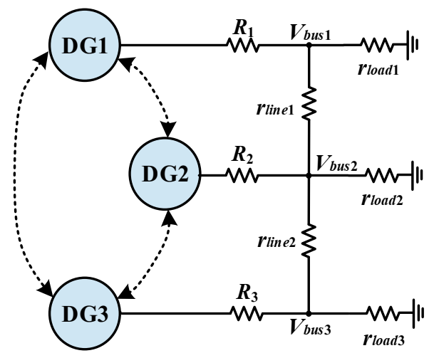
Figure 1. Hierarchical control structure for DC microgrid.
Processes 09 01992 g001
Figure 2. Schematic diagram of clock triggering process.
Processes 09 01992 g002
Figure 3. Network structure.
Processes 09 01992 g003
Figure 4. Periodicity in the sampling time offset during information interaction.
Processes 09 01992 g004
Figure 5. Control diagram for the proposed dynamic consensus algorithm.
Processes 09 01992 g005
Figure 6. Structure of the test DC microgrid.
Processes 09 01992 g006
Figure 7. (a) Evaluation of T3 when T1 and T2 are fixed. (b) Evaluation of T2 when T1 and T3 are fixed. (c) Evaluation of T1 when T2 and T3 are fixed. (d) Stability region of sampling periods for T1, T2 and T3.
Processes 09 01992 g007
Figure 8. Simulations with different control periods. (a) T1, T2, T3 = 0.1 s. (b) T1 = 0.12 s, T2 = 0.16 s, T3 = 0.07 s. (c) T1 = 0.12 s, T2 = 0.16 s, T3 = 0.18 s. (d) T1 = 0.12 s, T2 = 0.16 s, T3 = 0.04 s.
Processes 09 01992 g008
Figure 9. Simulation results for asynchronous sampled system with conventional algorithm. (a) Active powers. (b) Average voltage. (c) Secondary control inputs.
Processes 09 01992 g009
Figure 10. Simulation results for asynchronous sampled system with proposed algorithm. (a) Active powers. (b) Average voltage. (c) Secondary control inputs.
Processes 09 01992 g010
Figure 11. Simulation results in case of load variation under proposed algorithm.
Processes 09 01992 g011
Figure 12. Simulation results in case of topology switch under proposed algorithm.
Processes 09 01992 g012
Table 1. Network and control parameters.
ParameterValueParameterValue
MG voltage800 VConnection impedances
DG power ratingsR1/R2/R30.15 Ω/0.3 Ω/0.4 Ω
DG1, DG2, DG3120 kWLine impedances
Voltage droop coefficientrline1/rline20.2 Ω
mP1, mP2, mP31 × 10−3 V/WLoad ratings
Control parametersrload160 Ω/5 Ω
ki1/kp16/0.5rload260 Ω/5 Ω
ki2/kp210/0.5rload380 Ω/15 Ω
ki33
Publisher’s Note: MDPI stays neutral with regard to jurisdictional claims in published maps and institutional affiliations.

