Article

Design and Implementation of Integral Backstepping Sliding Mode Control for Quadrotor Trajectory Tracking

1
Department of Electrical Engineering, National Sun Yat-sen University, Kaohsiung 80424, Taiwan
2
Graduate Institute Automation Technology, National Taipei University of Technology, Taipei 10608, Taiwan
3
High-Tech Facility Research Center, Department of Civil Engineering, National Taiwan University, Zhubei 30264, Taiwan
*
Author to whom correspondence should be addressed.
Processes 2021, 9(11), 1951; https://doi.org/10.3390/pr9111951
Submission received: 5 October 2021 / Revised: 20 October 2021 / Accepted: 26 October 2021 / Published: 30 October 2021
(This article belongs to the Section Process Control and Monitoring)

Abstract

:
A robust trajectory tracking control scheme for quadrotor unmanned aircraft vehicles under uncertainties is proposed herein. A tracking controller combined with the sliding mode and integral backstepping is performed for position and attitude tracking. The stability of the trajectory tracking controller of the quadrotor is investigated via Lyapunov stability analysis. By incorporating force and torque disturbances into numerical simulations, the results demonstrate the effectiveness of the proposed quadrotor trajectory controller. Finally, the experiments validate the feasibility of the proposed controller.

1. Introduction

Recently, the rapid development of unmanned aircraft vehicles (UAVs) has received significant attention in various applications, such as search-and-rescue, safety inspections for civil buildings, agriculture, and forest surveillance. Different types of UAVs exist, including those that can take-off and land vertically in limited spaces, as well as those that can easily hover over the desired target. Compared with a helicopter, a quadrotor is typically constructed using a symmetrical lightweight airframe, with four brushless direction current (BLDC) motors mounted on it, and four fixed-pitch propellers attached to the respective motors. A quadrotor offers better mobility in attitude change and path planning compared with helicopters. However, the design of the flight controller of a quadrotor is associated with at least two challenges. First, the quadrotor is a multiple-input multiple-output (MIMO) unstable nonlinear system. Second, quadrotors, similar to other types of UAVs, are always subjected to external and internal disturbances, model uncertainties, and parametric perturbation. Therefore, they are difficult to control accurately in terms of trajectory tracking. Hence, the design and implementation of a stable and robust quadrotor flight controller are essential [1].
Proportional–integral–derivative (PID) control is a typical control technique that is typically used in industry. PID control involves many iterative trials for adjusting the parameters of the PID controller [2]. In [3], a nonlinear PID-type controller for the total thrust and torques was applied to perform trajectory tracking and the authors derived the adjustment guidelines. Meanwhile, in terms of the design of the flight controller of a V-tail quadrotor, Castillo–Zamora et al. performed the comparisons of tracking capability among a proportional-derivative (PD) controller, PID controller, and sliding mode controller (SMC) [4]. In their study, the simulation results showed that the PD controller presented an error in the stable state that would not disappear. This can be problematic if an application with precision is required. Meanwhile, the SMC has a facile and rapid response that drives the quadrotor to converge to the desired point in space.
Model-based controllers have been shown to exhibit excellent performance in resolving nonlinear control system problems. Observer-based backstepping and SMC for the trajectory tracking of a quadrotor have been presented in many studies. In [5], the authors designed an extended state observer (ESO) to estimate unmeasurable states and external disturbances. Wind gust and actuator faults can be considered as lumped disturbances, the disturbance torque caused by lumped disturbances happen suddenly, and cannot be estimated by traditional ESO. In order to alleviate lumped disturbances, high-order ESO have been applied. Nevertheless, higher observer orders will lead to higher control gains with fixed bandwidth, which will in return excite the sensor noise and introduce them into the control loop. Shi D. et al. proposed the super-twisting based ESO (ST-ESO) to estimate and attenuate the impact of lumped disturbances in finite time. In the same study, the super-twisting based SMC (ST-SMC) is also designed as the feedback controller to drive the attitude angle and angular velocity to their desired value in finite time [6]. In [7], the nonlinear disturbance observer (NDO) was used to compensate the disturbances and model-system errors. A backstepping SMC and observer-based fault estimation for a quadrotor was proposed in [8], where a regular SMC was used for attitude control, and the backstepping SMC was utilized for position and yaw angle control. An observer-based fault estimation serves as an alarming module as well as provides an estimation of faults occurring during the take-off and hovering modes. In the same paper, a stability analysis of the overall system based on the Lyapunov stability theory was presented.
Actuator dynamics, including transient responses and control input constraints, directly affect and limit the torque inputs to the propeller rotation of a quadrotor. It is risky to design the controller when the actuator saturation situation is omitted. By incorporating the SMC and dynamic surface controller (DSC) into a backstepping-like framework, the authors of [9,10] proposed a backpropagating constraint-based controller to solve the constrained actuator dynamics problem.
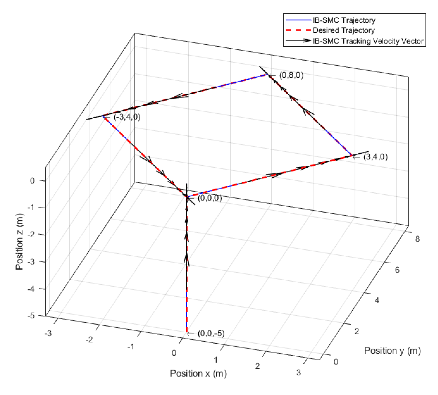
The contribution of this study is the design and implementation of an integral backstepping sliding mode controller (IB-SMC) of a quadrotor for real-time trajectory tracking [11,12]. For the hardware design of the quadrotor, we used a PX4 module as the flight control board; it contains six degree-of-freedom (DOF) inertial measurement unit (IMU) sensors, i.e., a three-axis accelerometer and a three-axis gyroscope [13]. A global positioning system (GPS) was used as the position estimator of the quadrotor. A radio frequency (RF) module was utilized to receive the control commands of the quadrotor from the user. The remainder of this paper is organized as follows: Section 2 presents the kinematics and dynamical model of the quadrotor. In Section 3, the design and stability analysis of the IB-SMC for the quadrotor are discussed. Section 4 provides the simulations and experimental results of the IB-SMC of the quadrotor. The conclusions are presented in Section 5.

2. Quadrotor Model

In navigation, guidance, and control of an aircraft or rotorcraft applications, several frame systems are used in design and analysis. These frame systems are the geodetic frame system, the earth-centered earth-fixed (ECEF) frame system, the local north-east-down (NED) frame system, the vehicle-carried NED frame system, and the body-fixed frame system. The geodetic frame system is widely used in GPS-based navigation. A coordinate point near the earth’s surface is characterized by longitude, latitude, and height. The ECEF frame system rotates with the earth around its spin axis, the origin of the ECEF frame system is located at the center of the earth. The local NED frame system is known as a navigation or ground coordinate system. It is a coordinate frame fixed to the earth’s surface and the origin of the local NED frame system is arbitrarily fixed to a point on the earth’s surface. The local NED frame plays an important role in flight control and navigation. Navigation of small-scale UAVs rotorcraft is normally carried out with this frame. The vehicle-carried NED frame system is associated with the flying vehicle and the origin of the vehicle-carried NED frame system is located at the center of gravity of the flying vehicle. The body-fixed frame system is vehicle-carried and is directly defined on the body of the flying vehicle. The origin of the body-fixed frame system is located at the center of gravity of the flying vehicle. The six DOFs IMU sensor is intensively used to capturing the rigid-body dynamics of unmanned systems [14]. Due to the inherent mechanical design and power limitation of quadrotor, the applications of quadrotor are normally operated at low speeds in small regions, so the local NED frame and the body-fixed frame are considered in this article.
The structure of the quadrotor is depicted in Figure 1a; the quadrotor has six DOFs and four control inputs. The six DOFs include translational motion in three directions and rotational motion around the three axes. Four rotors driven by a motor were mounted at the endpoint of two cross-shaped frames [8].
To establish a mathematical model for the quadrotor, it is assumed that the quadrotor frame is a symmetric grid body, the center of mass is at the geometric center of the body, and the flapping dynamics of the frame are negligible. For describing the attitude and position of the quadrotor, the local NED frame, i.e., the inertial frame, and the body-fixed frame are introduced. The inertial frame denoted as E = ( X E , Y E , Z E ) and the body-fixed frame denoted as B = ( X B , Y B , Z B ) . The inertial frame is based on the Earth with its origin coinciding with the origin of the body-fixed frame prior to take-off. Frame B is fixed with the quadrotor, and the origin of frame B is at the center of mass of the body.

2.1. Kinematics

The linear position vectors of the quadrotor expressed in the inertial frame E and body-fixed frame B are P E = [ x E y E z E ] T and P B = [ x B y B z B ] T , respectively. The attitude representation can be described by the quaternions and the Euler angles. The advantages of the Euler angles are an intuitive way to represent the attitude and their physical meanings are quite clear. Based on Euler’s theorem, the rotation of a rigid body around one fixed point can be regarded as the composition of several finite rotations around the fixed point. Recently, quaternions are getting more and more attention due to the wide application of high-performance computer and the rapid development of the aircraft’s attitude control technologies [15].
As shown in Figure 1b, the attitude (i.e., angular position) of the quadrotor defined in frame E is described by three Euler angles η E = [ ϕ θ ψ ] T , where ϕ , θ , and ψ denote the angles of roll, pitch, and yaw, respectively. ϕ is the angle between planes X E Y E and X B Y B , θ is the angle between planes Y E Z E and Y B Z B , and ψ is the angle between planes Z E X E and Z B X B . The angular velocity vector of the quadrotor is expressed as η ˙ E = [ ϕ ˙ θ ˙ ψ ˙ ] T . It is assumed that all attitude angles are limited between ( π 2 , π 2 ) . The linear position transformed from frame E to frame B is expressed as P B = R E B P E , where the rotation matrix R E B is written as follows:
R E B = [ cos θ cos ψ cos θ sin ψ sin θ sin ϕ sin θ cos ψ cos ϕ sin ψ sin ϕ sin θ sin ψ + cos ϕ cos ψ sin ϕ cos θ cos ϕ sin θ cos ψ + sin ϕ sin ψ cos ϕ sin θ sin ψ sin ϕ cos ψ cos ϕ cos θ ]  
If R E B is nonsingular, then the rotation matrix R E B is an orthogonal matrix, and the inverse matrix ( R E B ) 1 is obtained via a simple transpose, i.e., ( R E B ) 1 = ( R E B ) T . Hence, the linear position is transformed from frame B to frame E, expressed as P E = ( R E B ) T P B = R B E P B .
Three-axis gyroscopes are generally used in the aerospace industry to measure body rotations. The relationship between time rates of change of the Euler angles and the body axis angular rates are required. Assume that the angular velocity of the quadrotor with respect to frame B is ω B = [ p q r ] T , where p , q , and r are the angular velocities of the roll, pitch, and yaw, respectively. Therefore, the transformation matrix W E B for the angular velocity from frame E to frame B is written as
ω B = [ p q r ] = W E B η ˙ E = [ 1 0 sin θ 0 cos ϕ cos θ sin ϕ 0 sin ϕ cos θ cos ϕ ] [ ϕ ˙ θ ˙ ψ ˙ ]  
The angular velocity from the body-fixed frame to the inertial frame is expressed as [16,17,18,19].
η ˙ E = [ ϕ ˙ θ ˙ ψ ˙ ] = ( W E B ) - 1 ω B = [ 1 sin ϕ tan θ cos ϕ tan θ 0 cos ϕ sin ϕ 0 sin ϕ cos θ cos ϕ cos θ ] [ p q r ]
When the quadrotor executes many angular motions with low amplitude, ω B can be assimilated to [ ϕ ˙ θ ˙ ψ ˙ ] T .

2.2. Dynamics

Newton’s translational motion equation and Euler’s rotational motion equation are used to describe the dynamics of a quadrotor.

2.2.1. Translational Dynamics

As depicted in Figure 1a, the speed Ω i of the rotor R i generates a force F i in the direction of the rotor axis and creates a torque M i around the rotor axis. Hence,
F i = k t Ω i 2   and   M i = k d Ω i 2 ,
where k t is the thrust coefficient, and k d is the drag force coefficient. The thrust T in the z-axis direction of the body is obtained by the combined effect of forces generated by the four motors.
T = i = 1 4 F i = k t i = 1 4 Ω i 2
Subsequently, the thrust vector T B of the quadrotor with respect to frame B is written as
T B = [ F x B F y B F z B ] = [ 0 0 T ]
The moment is generated by creating a differential thrust across the two motors on the same arm of the quadrotor. M B is defined as the rotational torque provided by the four rotors with respect to frame B.
M B = [ M ϕ B M θ B M ψ B ] = [ d k t ( Ω 4 2 Ω 2 2 ) d k t ( Ω 3 2 Ω 1 2 ) k d ( Ω 2 2 + Ω 4 2 Ω 1 2 Ω 3 2 ) ] ,
where d is the distance between the center of the mass and the axis of the propeller. Based on Equation (7), the roll movement is obtained by decreasing the rotor velocity of the second motor and increasing the rotor velocity of the fourth motor. The pitch movement is obtained by decreasing the first rotor velocity and increasing the third rotor velocity. The yaw movement is obtained by increasing the angular velocities of the two opposite rotors and decreasing the velocities of the other two rotors [17]. Combining Equations (6) and (7), the matrix in Equation (8) shows the relationships among the vertical thrust F z B along the z-axis, rotational torques associated with the thrust difference of each rotor pair, i.e., M ϕ B , M θ B and M ψ B , and the angular velocities of the four propellers.
[ F z B M ϕ B M θ B M ψ B ] = [ k t k t k t k t 0 d k t 0 d k t d k t 0 d k t 0 k d k d k d k d ] [ Ω 1 2 Ω 2 2 Ω 3 2 Ω 4 2 ]
According to Newton’s second law of motion, the translational dynamics model of the quadrotor in frame E is expressed as follows:
V ˙ E = 1 m ( R B E T B G E F d ) ,
where V E = [ x ˙ E y ˙ E z ˙ E ] T is the linear velocity along the three axes in the inertial frame; m is the total mass of the quadrotor; R B E is the rotation matrix derived from Equation (1); T B is the lift force from Equation (6); G E = [ 0 0 m g ] T is gravity, where g is the acceleration due to gravity; F d = [ k 1 x ˙ k 2 y ˙ k 3 z ˙ ] T is the drag force caused by translational motions of the quadrotor, where, k 1 , k 2 and k 3 are the air drag coefficients. Substituting Equations (1) and (6) into Equation (9) yields
[ x ¨ E y ¨ E z ¨ E ] = 1 m ( R B E T B ) g [ 0 0 1 ] 1 m [ k 1 x ˙ k 2 y ˙ k 3 z ˙ ] = T m [ cos ϕ sin θ cos ψ + sin ϕ sin ψ cos ϕ sin θ sin ψ sin ϕ cos ψ cos ϕ cos θ ] g [ 0 0 1 ] 1 m [ k 1 x ˙ k 2 y ˙ k 3 z ˙ ]
Using Equations (6) and (10), we can extract the expressions for the pitch angle, roll angle, and thrust T, as follows:
ϕ E = sin 1 ( ( x ¨ E + k 1 m x ˙ E ) sin ψ ( y ¨ E + k 2 m y ˙ E ) cos ψ ( x ¨ E + k 1 m x ˙ E ) 2 + ( y ¨ E + k 2 m y ˙ E ) 2 + ( z ¨ E + g + k 3 m z ˙ E ) 2 )
θ E = tan 1 ( ( x ¨ E + k 1 m x ˙ E ) cos ψ + ( y ¨ E + k 2 m y ˙ E ) sin ψ ( z ¨ E + g + k 3 m z ˙ E ) )
T = m [ ( x ¨ E + k 1 m x ˙ E ) ( cos ϕ sin θ cos ψ + sin ϕ sin ψ ) + ( y ¨ E + k 2 m y ˙ E ) ( cos ϕ sin θ sin ψ sin ϕ cos ψ ) + ( z ¨ E + g + k 3 m z ˙ E ) ( cos ϕ cos θ ) ]

2.2.2. Rotational Dynamics

The quadrotor is a symmetric structure with four arms aligned with the body’s x- and y-axes. Based on Euler’s second law of motion, the rotational dynamics model of the quadrotor in frame B is expressed as follows:
ω ˙ B = ( I B ) 1 [ ( M B ω B × ( I B ω B ) M g M d ]
where M B is the torque in Equation (7); I B is the symmetric positive definite constant matrix expressed in Equation (15); I B ω ˙ is the angular acceleration of the inertia; ω × ( I B ω ) is the centripetal force, where the notation × denotes the cross product; M g is the resultant torque due to gyroscopic effects; M d is the resultant aerodynamic friction torque. The expressions for M g and M d are shown in Equation (16) and Equation (17), respectively [8,17,18,20,21].
I B = [ I x 0 0 0 I y 0 0 0 I z ]
M g = i = 1 4 ω × I r [ 0 0 ( 1 ) i + 1 Ω i ] T
M d = [ k 4 0 0 0 k 5 0 0 0 k 6 ] [ ϕ ˙ θ ˙ ψ ˙ ] = [ k 4 ϕ ˙ k 5 θ ˙ k 6 ψ ˙ ]
where I x , I y , and I z in Equation (15) are the rotary inertia for the x-, y-, and z-axes of the body, respectively; I r in Equation (16) is the moment of inertia of each rotor; k 4 , k 5 , and k 6 in Equation (17) are the aerodynamic drag coefficients.
Considering that I B is nonsingular and substituting Equations (16) and (17) into Equation (14), we obtain
ω ˙ B = [ p ˙ q ˙ r ˙ ] = ( I B ) 1 ( M B ω B × ( I B ω B ) M g M d ) = ( I B ) 1 ( M B [ p q r ] × [ I x p I y q I z r ] I r [ p q r ] × [ 0 0 1 ] Ω Γ [ k 4 ϕ ˙ k 5 θ ˙ k 6 ψ ˙ ] ) , = [ M ϕ B I x M θ B I y M ψ B I z ] + [ ( I y I z ) q r I x ( I z I x ) p r I y ( I x I y ) p q I z ] I r [ q I x p I y 0 ] Ω Γ [ k 4 ϕ ˙ I x k 5 θ ˙ I y k 6 ψ ˙ I z ]
where Ω Γ = Ω 4 + Ω 3 Ω 2 Ω 1 represents the overall speed of the quadrotor rotor. As shown in Equation (3), the angular acceleration vector in frame E is obtained from the angular acceleration in frame B comprising the transformation matrix, ( W E B ) 1 , and its time derivative is expressed as
η ¨ E = [ ϕ ¨ θ ¨ ψ ¨ ] = d d t [ ( W E B ) 1 ω B ] = [ d d t ( W E B ) 1 ] ω B + ( W E B ) 1 ω ˙ B
By substituting Equations (3) and (18) into Equation (19), we obtain
η ¨ E = [ ϕ ¨ θ ¨ ψ ¨ ] = [ ( I y I z ) θ ˙ ψ ˙ I x ( I z I x ) ϕ ˙ ψ ˙ I y ( I x I y ) ϕ ˙ θ ˙ I z ] I r [ θ ˙ I x ϕ ˙ I y 0 ] Ω Τ + [ M ϕ B I x M θ B I y M ψ B I z ] [ k 4 I x ϕ ˙ k 5 I y θ ˙ k 6 I z ψ ˙ ]

2.3. Model Simplification

The motions of the quadrotor are generated by combining a series of forces and moments from different physical effects. The model developed using Equations (10) and (20) describes the differential equation of the quadrotor system. In order to implement the flight controller in the resource limited microcontroller and consider the requirements of the dynamic response for the attitude controller which is 4 to 10 times faster than that of the position controller, it is assumed that the quadrotor is operated in a hovering state, so the models of quadrotor are linearized and the high-order effects of the force and moment models of the quadrotor can be simplified. Hence, the drag force F d in Equation (9) and the aerodynamic friction torque M d in Equation (14) were disregarded, and the thrust coefficient k t and drag force coefficient k d in Equation (4) were assumed to be constants [20]. The quadrotor system can be rewritten in the state-space form X ˙ = f ( X , U ) . The following input vector U and state vector X were selected:
X = [ x 1 x 2 x 3 x 4 x 5 x 6 x 7 x 8 x 9 x 10 x 11 x 12 ] T = [ ϕ ϕ ˙ θ θ ˙ ψ ψ ˙ x x ˙ y y ˙ z z ˙ ] T
U = [ U 1 U 2 U 3 U 4 ] = [ F z B M ϕ B M θ B M ψ B ]
The state representations of the system expressed in Equations (10) and (20) were simplified to the following
{ x 1 = ϕ x 2 = x ˙ 1 = ϕ ˙ x 3 = θ x 4 = x ˙ 3 = θ ˙ , x 5 = ψ x 6 = x ˙ 5 = ψ ˙ { x 7 = x x 8 = x ˙ 7 = x ˙ x 9 = y x 10 = x ˙ 9 = y ˙ x 11 = z x 12 = x ˙ 11 = z ˙
f ( X , U ) = [ ϕ ˙ ϕ ¨ θ ˙ θ ¨ ψ ˙ ψ ¨ x ˙ x ¨ y ˙ y ¨ z ˙ z ¨ ] = [ ϕ ˙ θ ˙ ψ ˙ a 1 θ ˙ a 2 Ω Τ + b 1 U 2 θ ˙ ϕ ˙ ψ ˙ a 3 + ϕ ˙ a 4 Ω Τ + b 2 U 3 ψ ˙ ϕ ˙ θ ˙ a 5 + b 3 U 4 x ˙ u x 1 m U 1 y ˙ u y 1 m U 1 z ˙ u z 1 m U 1 g ]
{ a 1 = ( I y I z ) I x a 2 = I r I x a 3 = ( I z I x ) I y a 4 = I r I y a 5 = ( I x I y ) I z , { b 1 = 1 I x b 2 = 1 I y b 3 = 1 I z , { u x = cos ϕ sin θ cos ψ + sin ϕ sin ψ u y = cos ϕ sin θ sin ψ sin ϕ cos ψ u z = cos ϕ cos θ
Subsequently, Equations (11) and (13) can be rewritten as
ϕ E = sin 1 ( x ¨ E sin ψ y ¨ E cos ψ ( x ¨ E ) 2 + ( y ¨ E ) 2 + ( z ¨ E + g ) 2 )
θ E = tan 1 ( x ¨ E cos ψ + y ¨ E sin ψ z ¨ E + g )
T = m [ x ¨ E u x + y ¨ E u + y ( z ¨ E + g ) u z ]
The revolutions per minute (rpm) to throttle conversion between the angular velocity of the rotors and the inputs is written as
[ Ω 1 2 Ω 2 2 Ω 3 2 Ω 4 2 ] = [ 1 4 k t 0 1 2 d k t 1 4 k d 1 4 k t 1 2 d k t 0 1 4 k d 1 4 k t 0 1 2 d k t 1 4 k d 1 4 k t 1 2 d k t 0 1 4 k d ] [ U 1 U 2 U 3 U 4 ]

3. Quadrotor Control

The SMC switches between two structures and causes the system states to approach the sliding surface. This sliding surface is defined over the state space or the error state space of the system. During the design of the SMC, a Lyapunov function was used to derive the stability of the system. The backstepping control approach sets a Lyapunov function and results in a stabilizing control law. The backstepping controller allows the entire system to be segregated into small subsystems. An error or regulatory variable is defined based on the designed Lyapunov function for each subsystem. Subsequently, a virtual control law is applied such that the subsystem is equivalent to a linear system and the derivative of the Lyapunov function is negative definite to ensure the stability of the system. However, the backstepping controller is not robust to parametric variations. To design a robust controller against matched and mismatched uncertainties, an integrator backstepping controller and an SMC are combined to achieve a continuous controlled signal, thereby eliminating the chattering effect from the control input [11].

3.1. Control Architecture

The system structure of a quadrotor is shown in Figure 2. The external uncertainties D = [ d 1 d 2 ] T are considered, where d 1 and d 2 represent the force and torque disturbances, respectively. The general form of the IB-SMC that reflects the dynamics of the quadrotor is shown in Figure 3. The backstepping controller is used to control the first subsystem and the SMC is utilized to control the second subsystem.

3.2. Attitude Tracking Control

As shown in Figure 2, the rotational controller is designed to ensure the trajectory tracking capability of the current pitch angle ϕ c E ( t ) , roll angle, θ c E ( t ) and yaw angle ψ c E ( t ) of the body along the desired pitch angle ϕ d E ( t ) , roll angle, θ d E ( t ) and yaw angle ψ d E ( t ) , respectively. Consider the first subsystem of the rotational controller with virtual control input α 1 as follows:
η ˙ E = α 1
The angle tracking error e 1 of the first subsystem is defined as
e 1 = η d E η E + J 1 ( η d E η E ) d t ,
where e 1 R 3 × 1 and J 1 R 3 × 3 are positive definite diagonal integral coefficient matrices. A backstepping controller was used to control the first subsystem. A Lyapunov function V 1 ( t ) = 1 2 e 1 T e 1 was considered for the first subsystem, and the time derivative of V 1 ( t ) is expressed as
V ˙ 1 ( t ) = e 1 T e ˙ 1 = e 1 T [ η ˙ d E η ˙ E + J 1 ( η d E η E ) ] = e 1 T [ η ˙ d E α 1 + J 1 ( η d E η E ) ]
The stabilization of the first subsystem can be obtained by designing the virtual control signal α 1 as follows:
α 1 = η ˙ d E + A 1 e 1 + J 1 ( η d E η E ) ,
where A 1 R 3 × 3 is a positive-definite diagonal matrix. Substituting Equation (33) into Equation (32), we obtain
V ˙ 1 ( t ) = e 1 T A 1 e 1 < 0 , e 1 0
Considering the simplified version of Equation (14) discussed in Section 2.3 and the torque disturbance d 2 , the second subsystem with virtual control input α 2 can be defined as
ω ˙ B = ( I B ) 1 α 2 f ( ω B ) + ( I B ) 1 d 2
where α 2 R 3 × 1 and f ( ω B ) are expressed as
{ f ( ω B ) = ( I B ) 1 [ ω B × ( I B ω B ) ] α 2 = M B M g
The SMC was used to control the second subsystem, and the angle-tracking error e 2 of the second subsystem is defined as
e 2 = α 1 η ˙ E
Next, the sliding surface S 1 is expressed as
S 1 = e ˙ 1 + A 1 e 1 = ( η ˙ d E η ˙ E ) + J 1 ( η d E η E ) + A 1 e 1 = α 1 η ˙ E = e 2
A Lyapunov function V 2 ( t ) = V 1 ( t ) + 1 2 S 1 T S 1 was considered for the second subsystem. Combining Equations (34) and (38),the time derivative of V 2 ( t ) is written as
V ˙ 2 ( t ) = V ˙ 1 ( t ) + S 1 T S ˙ 1 = ( e 1 T A 1 e 1 ) + S 1 T ( e ¨ 1 + A 1 e ˙ 1 ) = ( e 1 T A 1 e 1 ) + S 1 T [ η ¨ d E + J 1 ( η ˙ d E η ˙ E ) + A 1 ( S 1 A 1 e 1 ) η ¨ E ] = ( e 1 T A 1 e 1 ) + S 1 T [ η ¨ d E + J 1 ( η ˙ d E η ˙ E ) + A 1 ( S 1 A 1 e 1 ) ( I B ) 1 α 2 + f ( ω B ) ( I B ) 1 d 2 ]
The second subsystem can be stabilized by designing the virtual control signal α 2 as follows:
α 2 = I B [ η ¨ d E + A 1 ( S 1 A 1 e 1 ) + J 1 ( η ˙ d E + S 1 α 1 ) + f ( ω B ) + ε 1 s a t ( S 1 ) + Q 1 S 1 ]
where ε 1 R + and Q 1 R 3 × 3 are the positive real number and positive definite diagonal matrix, respectively; s a t ( S ) is the saturation function of the sliding surface, defined as [12]
s a t ( S ) = { S S   S > Δ 0     S = 0 S S S < Δ ( S Δ S ) S o t h e r w i s e ,
where Δ is a positive constant. To improve the robustness of the rotational controller, it was assumed that ε 1 ( I B ) 1 d 2 . By substituting Equation (40) into Equation (39), we obtain
V ˙ 2 ( t ) = ( e 1 T A 1 e 1 ) S 1 T Q 1 S 1 S 1 T ε 1 s a t ( S 1 ) S 1 T ( I B ) 1 d 2 ( e 1 T A 1 e 1 ) S 1 T Q 1 S 1 ε 1 S 1 + ( I B ) 1 d 2 S 1 = ( e 1 T A 1 e 1 ) S 1 T Q 1 S 1 ( ε 1 ( I B ) 1 d 2 ) S 1 < 0 , e 1 0 , S 1 0
Based on Equations (34) and (42), the stability of the rotational controller of the quadrotor is globally asymptotically stable; hence, the attitude trajectory tracking capability is confirmed [12].

3.3. Position Tracking Control

As shown in Figure 2, the objective of the translational controller is to ensure the excellent tracking performance of the position and yaw angle along the desired reference path P d E = [ x d E ( t ) y d E ( t ) z d E ( t ) ] T and ψ d E ( t ) . The first subsystem of the translational controller with a virtual control input α 3 is defined as
P ˙ E = α 3
The second subsystem of the translational controller with a virtual control input α 4 and force disturbance d 1 is defined as
V ˙ E = α 4 + 1 m d 1
where α 4 = 1 m ( R B E T B G E ) . The position tracking error e 3 of the first subsystem is defined as
e 3 = P d E P E + J 2 ( P d E P E ) d t
where J 2 R 3 × 3 is a positive-definite diagonal matrix. A backstepping controller was used to control the first subsystem. A Lyapunov function V 3 ( t ) = 1 2 e 3 T e 3 was considered for the first subsystem, and the time derivative of V 3 ( t ) is written as
V ˙ 3 ( t ) = e 3 T e ˙ 3 = e 3 T [ P ˙ d E P ˙ E + J 2 ( P d E P E ) ] = e 3 T [ P ˙ d E α 3 + J 2 ( P d E P E ) ]
The first subsystem can be stabilized by designing the virtual control signal α 3 as
α 3 = P ˙ d E + A 2 e 3 + J 2 ( P d E P E )
where A 2 R 3 × 3 is a positive-definite diagonal matrix. Substituting Equation (47) into Equation (46) yields
V ˙ 3 ( t ) = e 3 T A 2 e 3 < 0 , e 3 0
The SMC was used to control the second subsystem, as shown in Equation (44), and the position tracking error e 4 of the second subsystem is defined as
e 4 = α 3 P ˙ E
The sliding surface S 2 is defined as
S 2 = e ˙ 3 + A 2 e 3 = P ˙ d E P ˙ E + J 2 ( P d E P E ) + A 2 e 3 = α 3 P ˙ E = e 4
A Lyapunov function V 4 ( t ) = V 3 ( t ) + 1 2 S 2 T S 2 was considered for the second subsystem. Combining Equations (48) and (50), the time derivative of V 4 ( t ) is expressed as
V ˙ 4 ( t ) = V ˙ 3 ( t ) + S 2 T S ˙ 2 = ( e 3 T A 2 e 3 ) + S 2 T ( α ˙ 3 P ¨ E ) = ( e 3 T A 2 e 3 ) + S 2 T [ P ¨ d E + A 2 ( S 2 A 2 e 3 ) + J 2 ( P ˙ d E P ˙ E ) α 2 1 m d 1 ]
The second subsystem can be stabilized by designing the virtual control signal α 4 as
α 4 = P ¨ d E + A 2 ( S 2 A 2 e 3 ) + J 2 ( P ˙ d E + S 2 α 3 ) + Q 2 S 2 + ε 2 s a t ( S 2 )
where ε 2 R + and Q 2 R 3 × 3 are the positive real number and positive definite diagonal matrix, respectively; s a t ( S ) is the saturation function of the sliding surface shown in Equation. (41). To improve the robustness of the controller, it was assumed that ε 2 1 m d 1 . By substituting Equation (52) into Equation (51), we obtain
V ˙ 4 ( t ) = ( e 3 T A 2 e 3 ) + S 2 T [ Q 2 S 2 ε 2 s a t ( S 2 ) 1 m d 1 ] ( e 3 T A 2 e 3 ) S 2 T Q 2 S ε 2 S 2 + 1 m d 1 S 2 = ( e 3 T A 2 e 3 ) S 2 T Q 2 S ( ε 2 1 m d 1 ) S 2 < 0 , e 3 0 , S 2 0
The combination of Equations (48) and (53) indicates that the stability of the translational controller of the quadrotor is globally asymptotically stable, and that positional trajectory tracking capability is confirmed [12].

4. Simulations and Experimental Results

In this section, numerical simulations and experiments for trajectory tracking were implemented to validate the merit and effectiveness of the IB-SMC of the quadrotor. By considering external disturbances, the trajectory tracking results, including those for take-off, hovering, and landing, are shown in Section 4.1. The simulations were conducted using the MATLAB & Simulink software tool, and the computations were performed on a personal computer with an Intel Core i5-8265 CPU, 16 GB of RAM, and an Nvidia Geforce MX110 graphical card. The trajectory tracking experiments for the IB-SMC of the quadrotor are explained in Section 4.2.

4.1. Simulations

The designs of the IB-SMC of the quadrotor for attitude control and position control described in Section 3 were simulated. For simplicity, the physical phenomenon presented in the real world, i.e., fluid dynamics, the friction of the four rotors, the error range from the GPS modules which are mounted on the quadrotor are ignored, therefore, the conceptual behavior for the trajectory tracking of the tracking controller in the real world are simulated. The parameters of the quadrotor model are listed in Table 1. The parameters of the quadrotor controllers are listed in Table 2. The initial states of the quadrotor were η E ( 0 ) = 0 , V E ( 0 ) = 0 , and ω B ( 0 ) = 0 .
To demonstrate the physical disturbance, the force d 1 and torque disturbance d 2 were assumed as the following:
{ d 1 = d 1 , s t a t i c + d 1 , r a n d o m 0   s t < 5   s d 2 = d 2 , s t a t i c + d 2 , r a n d o m 5   s t < 10   s
d 1 , s t a t i c = 0.25 [ 1 1 1 ] T , 0.05 [ 1 1 1 ] T d 1 , r a n d o m 0.05 [ 1 1 1 ] T d 2 , s t a t i c = 0.1 [ 1 1 1 ] T , 0.05 [ 1 1 1 ] T d 2 , r a n d o m 0.05 [ 1 1 1 ] T
Here, d i , s t a t i c ( i = 1 , 2 ) represents a slow change, and the unknown constant disturbances along with time d i , s t a t i c can be regarded as static wind or unmodeled dynamic errors; d i , r a n d o m ( i = 1 , 2 ) represents the fast varying and unknown stochastic disturbance with the assumption of a uniform distribution, and d i , r a n d o m can be regarded as stochastic wind or uncertain measurement noise; t is the simulation time [12].
To emulate the tracking performance of the quadrotor in the experiment, five trajectory paths were planned, as follows:
( x , y , z ) = { ( 0 ,   0 , 5 + 2.5 t ) ( 1.5 ( t 2 ) ,   2 ( t 2 ) ,   0 ) ( 3 1.5 ( t 4 ) ,   4 + 2 ( t 4 ) ,   0 ) ( 1.5 ( t 6 ) ,   8 2 ( t 6 ) ,   0 ) ( 3 + 1.5 ( t 8 ) ,   4 2 ( t 8 ) ,   0 ) 0   s t 2   s 2   s < t 4   s 4   s < t 6   s 6   s < t 8   s 8   s < t 10   s
The initial posture of the quadrotor was set to P 0 E ( t ) = P 0 E ( 0 ) = ( 0 , 0 , 5 ) at t = 0   s . Five target positions were set: the first position was located at P 1 E ( 2 ) = ( 0 , 0 , 0 ) at t = 2   s , the second position was P 2 E ( 4 ) = ( 3 , 4 , 0 ) , the third position was P 3 E ( 6 ) = ( 0 , 8 , 0 ) , the fourth position was P 4 E ( 8 ) = ( 3 , 4 , 0 ) ; Subsequently, the quadrotor returns to the final target position P 5 E ( 10 ) = ( 0 , 0 , 0 ) at t = 10   s . Figure 4 shows the tracking for the desired, IB-SMC trajectories and IB-SMC tracking velocity vector.
Figure 5a,c,e show the position response of the trajectory tracking presented in Figure 4. The position error between the desired and real trajectories with disturbance is shown in Figure 5b,d,f. At t = 5   s , the position errors in the x-, y-, and z-axes were −0.0009372, −0.001187, and −0.001044, respectively.
Figure 6a,c,e show the Euler’s angle response for the trajectory tracking. The Euler’s angle error between the desired and real trajectories under disturbance is shown in Figure 6b,d,f. As shown in these figures, when disturbance was considered, the developed IB-SMC enabled the attitude-tracking capability of the quadrotor.
As shown in Figure 7a, the value of the thrust T was 3.142 × 10 4 . However, owing to the physical limitation of the rotor, the speed of the rotor was limited; therefore, the real thrust was less than 3.142 × 10 4 . Figure 7b–d show the rotational torques M ϕ ,   M θ and M ψ , and the variation range of these rotational torques was from 0.05   N m to 0.15   N m . It was observed that the developed IB-SMC of the quadrotor was robust against disturbance.

4.2. Experiments

Figure 8 shows the prototype of the proposed quadrotor. The hardware components of the quadrotor are listed in Table 3.
In order to validate the path tracking performance of the proposed quadrotor, the original proportional-PID (P-PID) translational controller implemented in Pixhawk was replaced by the IB-SMC translational controller. Figure 9 shows the trajectory tracking plan in the experiment, where the tracking targets were set using the QGround control (QGC) software tool in the ground station. The experiments were performed at the stadium of the university. The tracking targets were denoted as P 1 , P 2 , P 3 and P 4 on the Google map. The original position was P 1 , which was located at ( 24 58 05.9   N ,   121 11 25.2   E ) ; P 2 was at ( 24 58 06.9   N ,   121 11 24.4   E ) , P 3 was at ( 24 58 06.1   N ,   121 11 23.8   E ) , and P 4 was at ( 24 58 05.5   N ,   121 11 24.5   E ) . The tracking path was from P 1 to P 4 , followed a return to P 1 by passing through P 2 and P 3 . The flight height of the quadrotor was set to 5 m.
The trajectory tracking processes of the quadrotor are shown in Figure 10a–e. The link to the video is provided in the Supplementary Material. The flight data of the quadrotor were obtained using the Pixhawk module and then transmitted via the RF module. Subsequently, these flight data were received by the ground station. Figure 11 shows the position response of the trajectory tracking in the experiment. As shown, the developed IB-SMC of the quadrotor can provide effectiveness trajectory tracking in the experiment.

5. Conclusions and Future Works

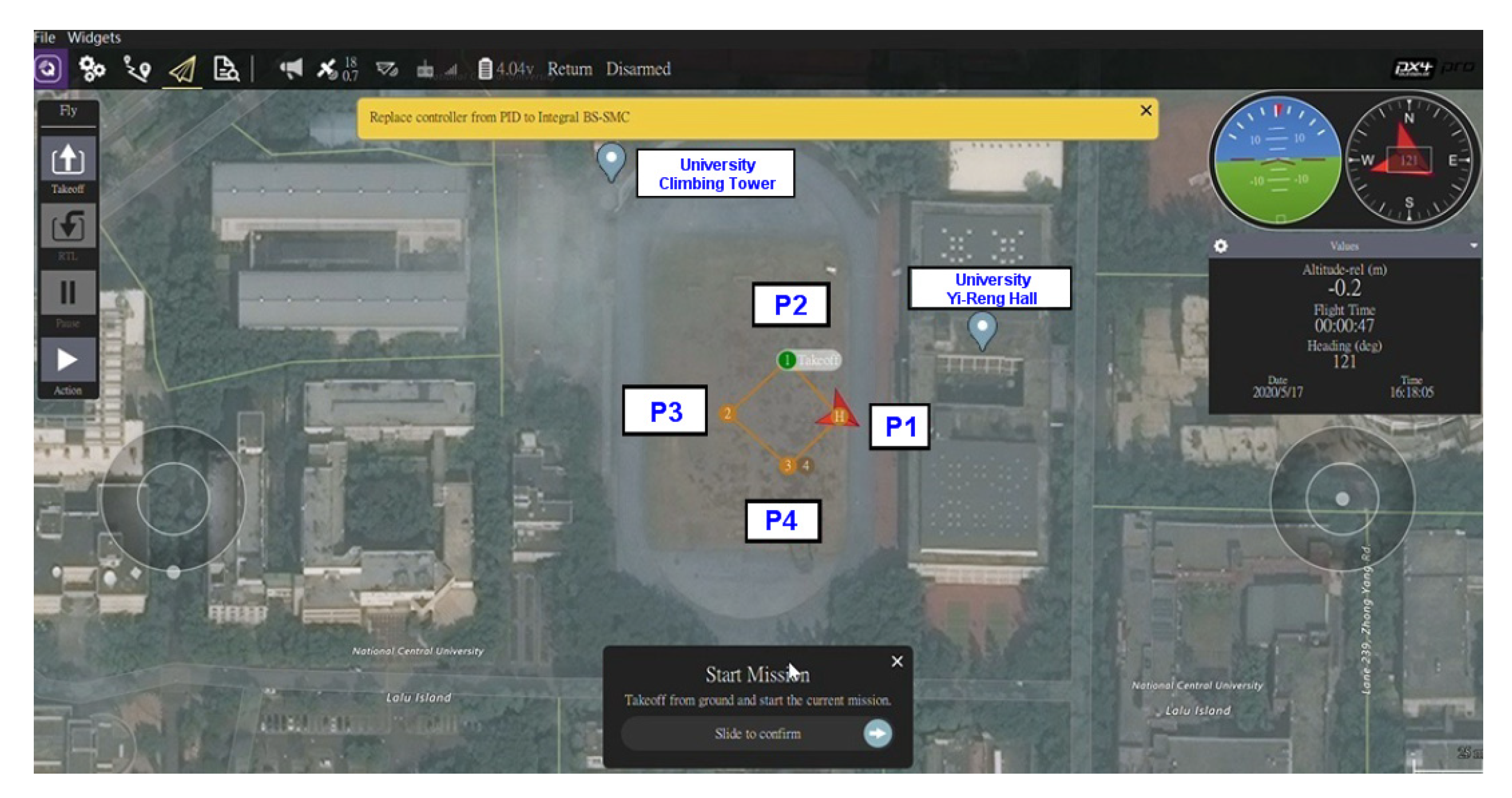
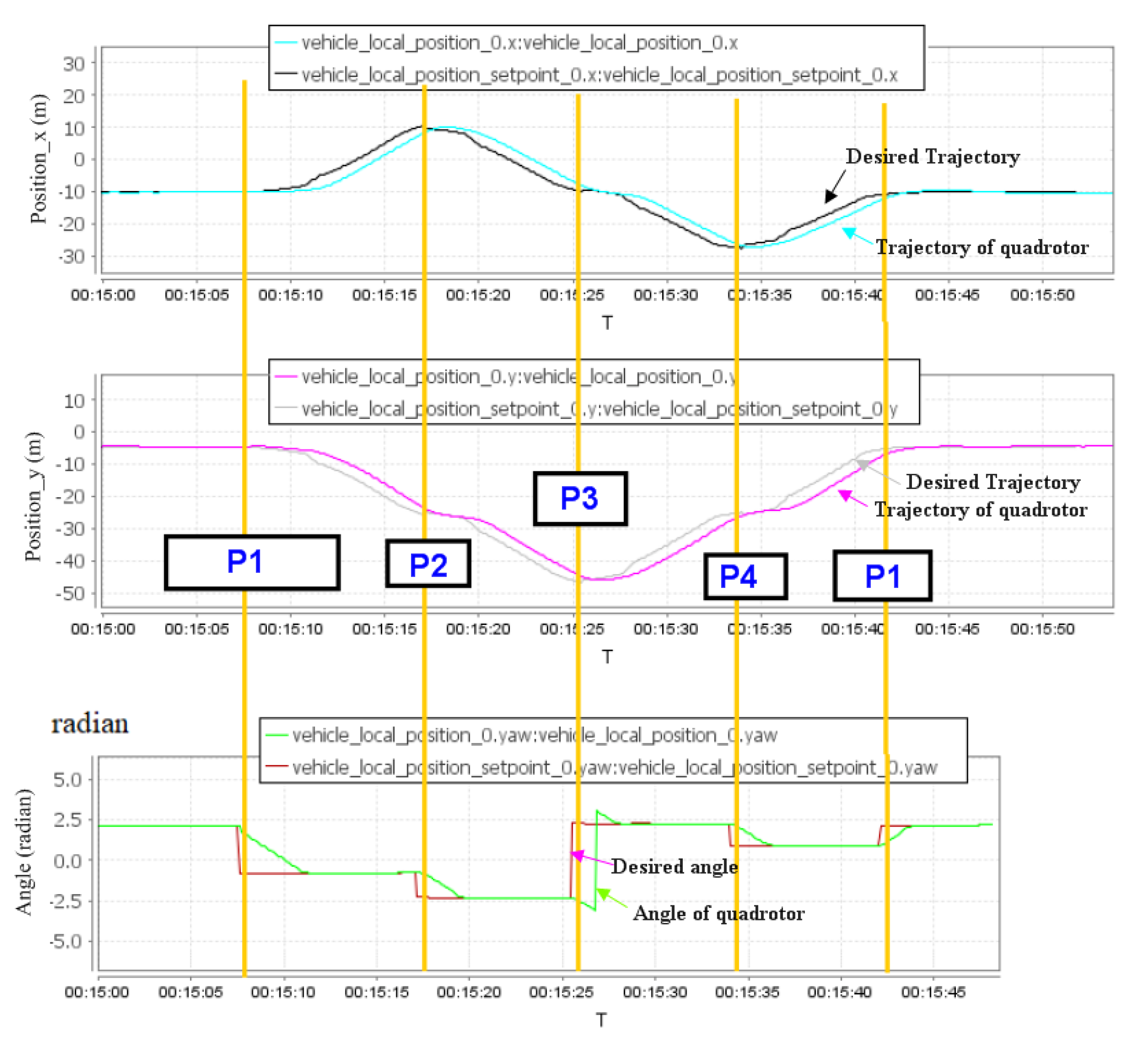
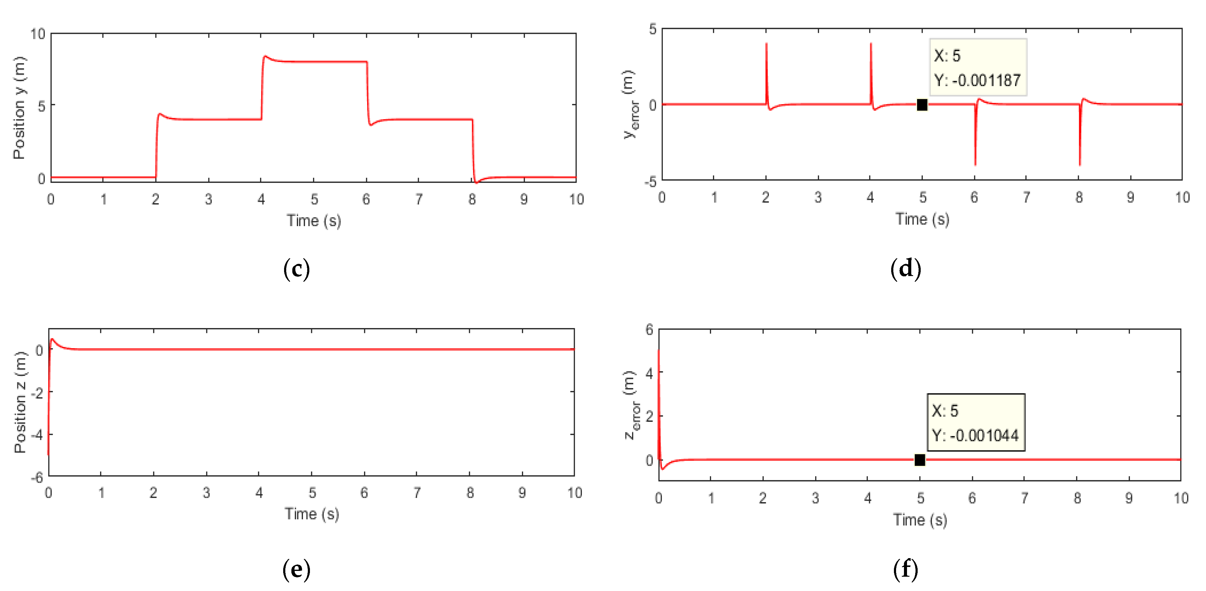
In this study, the design of the IB-SMC of a quadrotor for trajectory position tracking was investigated. A GPS and six-axis IMU sensors, which constituted the Pixhawk module, were utilized to measure the position and attitude of the quadrotor. Theoretical analysis and numerical simulations for designing the IB-SMC were provided. Finally, experiments were performed to validate the feasibility and effectiveness of the proposed IB-SMC for a quadrotor.
For designing the next generation of the quadrotor, the quadrotor with the capabilities of obstacle avoidance, slug-payload are two main research topics. For obstacle detection and collision avoidance approaches, the readouts of the ultrasonic sensor, millimeter-Wave (mmWave) radar sensor and Light-detection and ranging (LIDAR) sensor can be integrated by the multi-sensor fusion algorithm and then pattern recognition technologies are used to identify objects by utilizing the machine learning algorithms [22,23,24]. For aerial transportation applications, delivering cargo via quadrotor is a new trend. However, a quadrotor with a slug-payload system is an underactuated, strong coupling, and nonlinear system. How to achieve the quadrotor with precise positioning, maximum payload, and minimum oscillation of suspended load simultaneously needs be investigated in the future [25]. Moreover, for extending the operating time of quadrotor, power management strategies need to be carefully planned further.

Supplementary Materials

The following are available online at https://www.mdpi.com/article/10.3390/pr9111951/s1, Video S1.

Author Contributions

Conceptualization, S.-H.T.; Embedded program implementation, S.-H.T. and H.-Y.L.; Matlab program, Y.-P.C. and H.-Y.L.; Validation, S.-H.T. and L.-M.C.; Writing draft, H.-Y.L. and Y.-P.C.; Math Review, L.-M.C.; Funding, L.-M.C.; Literature Review, S.-H.T., H.-Y.L. and L.-M.C. All authors have read and agreed to the published version of the manuscript.

Funding

This work was supported by the Ministry of Science and Technology of Taiwan, under Grant MOST 110-2221-E-002-165, Grant MOST-110-2221-E-110-067, Grant MOST 109-2221-E-110-080, and Grant MOST 110-2811-E-002-561.

Acknowledgments

The authors also gratefully acknowledge the helpful comments and suggestions of the Editor and anonymous reviewers, which had improved the presentation of this paper.

Conflicts of Interest

The authors declare no conflict of interest.

References

  1. Almakhles, D.J. Robust backstepping sliding mode control for a quadrotor trajectory tracking application. IEEE Access 2020, 8, 5515–5525. [Google Scholar] [CrossRef]
  2. Golnaraghi, F.; Kuo, B.C. Automatic Control Systems, 9th ed.; Wiley: Hoboken, NJ, USA, 2009; pp. 528–532. [Google Scholar]
  3. Moreno-Valenzuela, J.; Pérez-Alcocer, R.; Guerrero-Medina, M.; Dzul, A. Nonlinear PID-type controller for quadrotor trajectory tracking. IEEE/ASME Trans. Mechatron. 2018, 23, 2436–2447. [Google Scholar] [CrossRef]
  4. Castillo-Zamora, J.J.; Camarillo-Gόmez K., A.; Pérez-Soto, G.I.; Rodríguez-Reséndiz, J. Comparison of PD, PID and sliding-mode position controllers for V-Tail quadcopter stability. IEEE Access 2018, 6, 38086–38096. [Google Scholar] [CrossRef]
  5. He, M.; He, J. Extended state observer-based robust backstepping sliding mode control for a small-size helicopter. IEEE Access 2018, 6, 33480–33488. [Google Scholar] [CrossRef]
  6. Shi, D.; Wu, Z.; Chou, W. Super-twisting extended state observer and sliding mode controller for quadrotor UAV attitude system in presence of wind gust and actuator faults. Electronics 2018, 7, 128. [Google Scholar] [CrossRef] [Green Version]
  7. Fethalla, N.; Saad, M.; Michalska, H.; Ghommam, J. Robust observer-based dynamic sliding mode controller for a quadrotor UAV. IEEE Access 2018, 6, 45846–45859. [Google Scholar] [CrossRef]
  8. Chen, F.; Jiang, R.; Zhang, K.; Jiang, B.; Tao, G. Robust backstepping sliding-mode control and observer-based fault estimation for a quadrotor UAV. IEEE Trans. Ind. Electron. 2016, 63, 5044–5056. [Google Scholar] [CrossRef]
  9. Zhu, Z.; Xia, Y.; Fu, M. Adaptive sliding mode control for attitude stabilization with actuator saturation. IEEE Trans. Ind. Electron. 2011, 58, 4898–4907. [Google Scholar] [CrossRef]
  10. Wang, N.; Su, S.-F.; Han, M.; Chen, W.-H. Backpropagating constraints-based trajectory tracking control of a quadrotor with constrained actuator dynamics and complex unknowns. IEEE Trans. Syst. Man. Cybern. Syst. 2019, 49, 1322–1337. [Google Scholar] [CrossRef]
  11. Adhikary, N.; Mahanta, C. Integral backstepping sliding mode control for underactuated system: Swing-up and stabilization of the cart-pendulum system. ISA Trans. 2013, 52, 870–880. [Google Scholar] [CrossRef] [PubMed]
  12. Jia, Z.; Yu, J.; Mei, Y.; Chen, Y.; Shen, Y.; Ai, X. Integral backstepping sliding mode control for quadrotor helicopter under external uncertain disturbances. Aerosp. Sci. Technol. 2017, 68, 299–307. [Google Scholar] [CrossRef]
  13. Moeini, A.; Rafique, M.A.; Xue, Z.; Lynch, A.F.; Zhao, Q. Disturbance observer-based integral backstepping control for UAVs. In Proceedings of the International Conference on Unmanned Aircraft Systems, Athens, Greece, 1–9 September 2020; pp. 382–388. [Google Scholar]
  14. Cal, G.; Chen, B.; Lee, T.H. Unmanned Rotorcraft Systems, 1st ed.; Springer: London, UK, 2011; pp. 23–34. [Google Scholar]
  15. Quan, Q. Introduction to Multicopter Design and Control, 1st ed.; Springer Nature: Singapore, 2017; pp. 99–120. [Google Scholar]
  16. Alderete, T.S. Simulation Aero Model Implementation. Available online: https://aviationsystems.arc.nasa.gov/publications/hitl/rtsim/Toms.pdf (accessed on 20 August 2021).
  17. Luukkonen, T. Modeling and Control of Quadrotor. Available online: https://www.mecharithm.com/wp-content/uploads/2020/11/quadrotor_dynamics.pdf (accessed on 20 August 2021).
  18. Kayacan, E.; Maslim, R. Type-2 fuzzy logic trajectory tracking control of quadrotor VTOL aircraft with elliptic membership function. IEEE/ASME Trans. Mechatron. 2017, 22, 339–348. [Google Scholar] [CrossRef]
  19. Antonelli, G.; Cataldi, E.; Arrichiello, F.; Giordano, P.R.; Chiaverini, S.; Franchi, A. Adaptive trajectory tracking for quadrotor MAVs in presence of parameter uncertainties and external disturbances. IEEE Trans. Control. Syst. Technol. 2018, 26, 248–254. [Google Scholar] [CrossRef]
  20. Bouabdallah, S. Design and Control of Quadrotors with Application to Autonomous Flying. Ph.D Thesis, École Polytechnique Fédéral de Lausanne, Lausanne, Switzerland, February 2007. [Google Scholar]
  21. Fay, G. Derivation of the Aerodynamic Forces for the Mesicopter Simulation. Available online: https://media.gradebuddy.com/documents/340594/59482841-8400-4d1d-890d-8932a64a24d1.pdf (accessed on 17 October 2021).
  22. Gageik, N.; Benz, P.; Montenegro, S. Obstacle detection and collision avoidance for a UAV wiith complementary low-cost sensors. IEEE Access 2015, 3, 599–609. [Google Scholar] [CrossRef]
  23. Safa, A.; Verbelen, T.; Keuninckx, L.; Ocket, I.; Hartmann, M.; Bourdoux, A.; Catthoor, F.; Gielen, G.G.E. A low-complexity radar detector outperforming OS-CFAR for indoor drone obstacle avoidance. IEEE J. Sel. Top. Appl. Earth Observ. Remote Sens. 2021, 14, 9162–9175. [Google Scholar] [CrossRef]
  24. Singla, A.; Padakandla, S.; Bhatnagar, S. Memory-based deep reinforcement learning for obstacle avoidance in UAV with limited environment knowledge. IEEE Trans. Intell. Transp. Syst. 2021, 22, 107–118. [Google Scholar] [CrossRef]
  25. Xian, B.; Wang, S.; Yang, S. An online trajectory planning approach for a quadrotor UAV with a slug payload. IEEE Trans. Ind. Electron. 2020, 67, 6669–6678. [Google Scholar] [CrossRef]
Figure 1. (a) Quadrotor configuration frame scheme comprising body-fixed and inertial frames. (b) Transfer of Euler angles from body-fixed frame to inertial reference frame.
Processes 09 01951 g001
Figure 2. Block diagram of control structure of quadrotor.
Processes 09 01951 g002
Figure 3. General form of IB-SMC reflecting dynamics of quadrotor.
Processes 09 01951 g003
Figure 4. Three-dimensional trajectory tracking with disturbance.
Processes 09 01951 g004
Figure 5. (a,c,e) Position response of quadrotor. (b,d,f) Position error between desired and real trajectories.
Processes 09 01951 g005aProcesses 09 01951 g005b
Figure 6. (a,c,e) Euler’s angle response of quadrotor. (b,d,f) Euler’s angle error between desired and real trajectories.
Processes 09 01951 g006
Figure 7. (a) Virtual control input: total thrust T. (bd) Rotational torques M ϕ , M θ , and M ψ .
Processes 09 01951 g007
Figure 8. Prototype of proposed quadrotor.
Processes 09 01951 g008
Figure 9. Tracking plan of quadrotor in experiment.
Processes 09 01951 g009
Figure 10. (ae) Trajectory tracking processes of quadrotor in experiment.
Processes 09 01951 g010aProcesses 09 01951 g010b
Figure 11. Position response of quadrotor in experiment.
Processes 09 01951 g011
Table 1. Model parameters of quadrotor.
SchemeValue (Units)SymbolValue (Unit)
m0.5 (kg)d0.2 (m)
I x 2.35 × 10 3 ( kg m 2 ) g 9.81 ( m / s 2 )
I y 2.35 × 10 3 ( kg m 2 ) k t 6.13 × 10 5 ( N s 2 )
I z 5.26 × 10 2 ( kg m 2 ) k d 2.5 × 10 6 ( N m s 2 )
Table 2. Controller parameters.
SymbolValue (Unit)SymbolValue (Unit)
A 1 1.5 I 3 × 3 A 2 9 I 3 × 3
ε 1 10 ε 2 2
Q 1 5 I 3 × 3 Q 2 50 I 3 × 3
J 1 3 I 3 × 3 J 2 0.9 I 3 × 3
Δ 5
Table 3. Hardware components quadrotor model parameters.
ComponentPart NameSpecifications
AirframeTarot FY450Diameter: 450 mm
Weight: 282 g
X-configuration skeleton
4 × BLDC motorsTarot2214–920 KV920 rpm/V
Maximum current: 10.3 A
Resistance :   180   Ω
Electric batteryATC Li–Po 3 CellsVoltage: 11.1 V
Capacity: 5200 mAh
GPS moduleNEO–M8NFrequency: 1575.42 MHz,
Transmission rate: 9600 bps
4 × propellers 10 × 4.52 blades (CC and CCW pair)
RF moduleRFD900Frequency: 902–928 MHz
Electronic speed controllerORun 30 APWM to PPM
Flight control modulePixhawkVersion: 2.4.8
Publisher’s Note: MDPI stays neutral with regard to jurisdictional claims in published maps and institutional affiliations.

