Mobile Emergency Power Source Configuration Scheme considering Dynamic Characteristics of a Transportation Network

Abstract

Recently, with the large scale of power grids and the increase in frequency of extreme weather, the safe and stable operation of power systems is facing great challenges. Therefore, mobile emergency power source (MEPS) are a promising and feasible way to deal with extreme weather and reduce economic losses. However, the current urban power grid and transportation network are closely coupled, and the congested traffic hinders the rapid configuration of MEPSs. Therefore, this paper proposes an MEPS configuration scheme considering real-time traffic conditions. Firstly, the dynamic road traffic index (DRTI) is defined, which can fully describe the dynamic characteristics of traffic. The wavelet neural network (WNN) is used to predict the traffic flow. Then, combined with the knowledge of graph theory, an A-Star algorithm (AS) is used to determine the optimal path. Secondly, the optimal installation location of MEPSs is determined by forward–backward sweep method in distribution network. Finally, the feasibility, accuracy, and time cost of the proposed method are verified by numerical simulations, which can meet the requirements of online application.

1. Introduction

With the development of economy and society, power systems play an increasingly important role, and have become the pillar of national economic development. Therefore, it is of great significance to guarantee the security and stable operation of a power system. However, some extreme weather, such as typhoons, hail, and cold tides will greatly affect the safety level of power systems. Extreme weather will damage the transmission line of the power grid, and even lead to the destruction of power equipment and voltage collapse of the whole system [1]. In addition, the load is mainly concentrated in the distribution network, especially the urban power grid [2], so the requirements for reliable power supply are more stringent. When an urban power system is in a great power outage caused by an extreme climate disaster [3,4], the daily life of residents will be greatly affected, and a large number of economic losses and serious consequences will occur at the same time. In addition, the impact of extreme weather on a distribution network is also reflected in other aspects. The large-scale trip of transmission and distribution lines and the collapse of towers are difficult to avoid. For example, on 12th August 2004, typhoon named Ranamin landed in Wenling of the Zhejiang Province, which posed a serious threat to the Zhejiang power grid and caused frequent and concentrated trip times of transmission lines over 220 kV. In mid-February 2021, Texas, USA experienced a once-in-a-century cold tide, with the lowest temperature 10–20 °C lower than that of the same period in the past year. The local power grid faced the most serious power supply crisis in history from 15 to 19 February, with large area and long-term power failure affecting more than 4 million families [5,6,7].

Although extreme weather is uncontrollable, with the development of information technology, the occurrence time and place of extreme weather, such as typhoons and cold tides, can be predicted in advance, so as to guide the relevant operators of power systems to implement risk aversion action and emergency repair. Relevant researchers have carried out some constructive and valuable research. The methods of the distribution network reconfiguration and the line reinforcement are adopted from literature [8,9,10], which yielded positive effects.

The above methods focus on power system control and dispatching; another effective way to meet the needs of urban power emergency support is to configure mobile emergency power sources (MEPSs) [11,12,13]. Mobile emergency power sources, i.e., the installation of power resources on large vehicles, provide high mobility, flexibility, and quick response to emergency events. As shown in Figure 1, the China National Grid Corporation has begun to use MEPSs to provide power supply in extreme weather scenarios, and has achieved remarkable results. MEPSs have become an important and fundamental means to improve the reliability of power systems and respond to various kinds of faults and disasters. Therefore, the power systems of modern cities are actively allocating MEPSs, which are listed as one of the most essential resources. A great deal of research about mobile emergency power source has been carried out and relevant methods are listed in

Table 1. Research about MEPSs and relevant methods.

References	Methods Adopted in the References
[14,15]	Two-stage restoration scheme is designed to facilitate the distribution system restoration following the high-impact low-probability (HILP) seismic disasters.
[16,17]	A post-event restoration framework for the distribution system in response to high impact low probable events is presented.
[18]	This paper proposes a service restoration method considering interdependency between the power distribution system and transportation system, which is formulated as a mixed-integer linear program (MILP).
[19]	This paper proposes an optimization model of a power emergency repair path under a typhoon disaster. It aims to deploy the repair team in advance, based on the advance prediction of the power outage.
[20]	This paper proposes a robust receding horizon recovery strategy that dispatches MEPSs and forms multiple microgrids (MGs) to maximize the restored critical loads (CLs).

.

However, some challenges still remain:

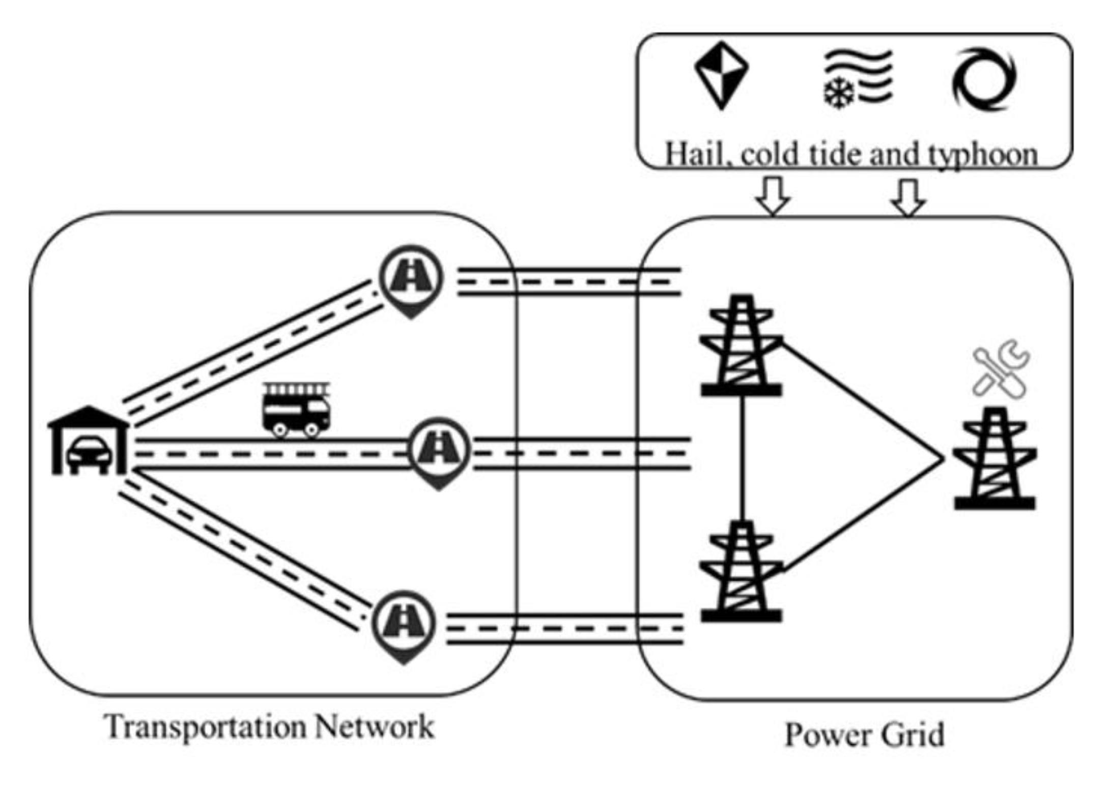
• First, as mentioned above, urban power grids and transportation networks are closely coupled, so MEPSs need to reach the fault location through the urban transportation network shown in Figure 2. However, when extreme weather occurs, it will affect the urban transportation network, such as cold tide weather leading to road icing, which makes it difficult for MEPS to reach the destination quickly. In addition, some static traffic planning methods are not optimal because they ignore the real-time traffic conditions and dynamic traffic flow.
• Secondly, the traditional path selection and determination algorithm, such as the Dijkstra algorithm and Warshall–Floyd algorithm, are still limited by the solution speed, which limits the online application. For urban traffic networks, there is an urgent need for an efficient path determination algorithm.

Thus, this paper proposes a novel MEPS configuration scheme considering dynamic characteristics of transportation networks, which decompose the original configuration problem into a two-stage problem. The first stage aims for the transportation network and determines the optimal route of MEPS; in the second stage, the aim is to determine the optimal accessing location of MEPS for urban power grid. The remainder of the paper is as follows: The concept of dynamic road traffic index (DRTI) is given in Section 2.1, which fully reflects the dynamic characteristics of the transportation network, such as traffic flow, route length and congestion time. In Section 2.2, the wavelet neural network (WNN) is used to predict traffic flow, and the mathematical model and corresponding calculation procedure of A-Star (AS) algorithm are introduced in Section 2.3. In the third section, the forward–backward sweep method is used to solve the distribution network power flow. On the premise of ensuring the power supply, the optimal installation location of MEPS is determined to minimize the power loss of the system. Finally, the performance of the proposed method is demonstrated in Section 4. The accuracy of the WNN, the feasibility of the AS algorithm and the efficiency of the forward–backward sweep method are verified by numerical simulations.

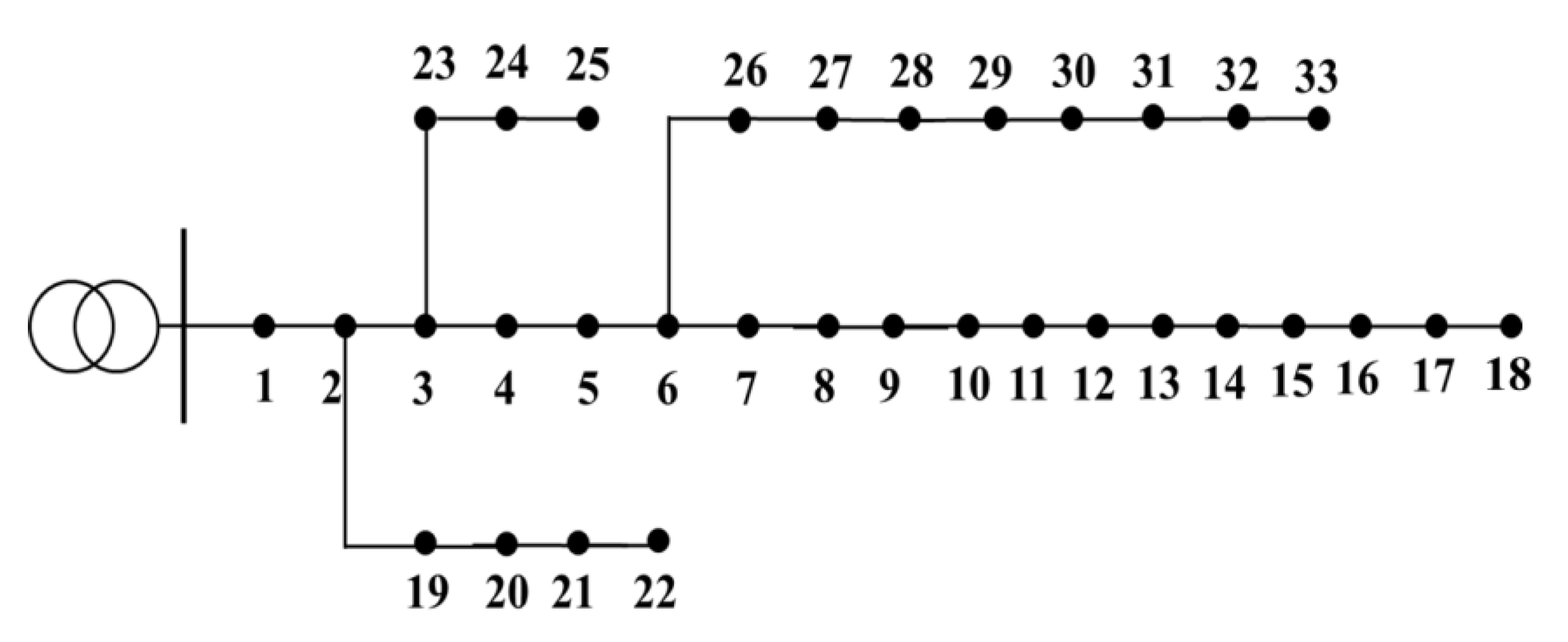
2. The Determination of Optimal Route in an Urban Transportation Network

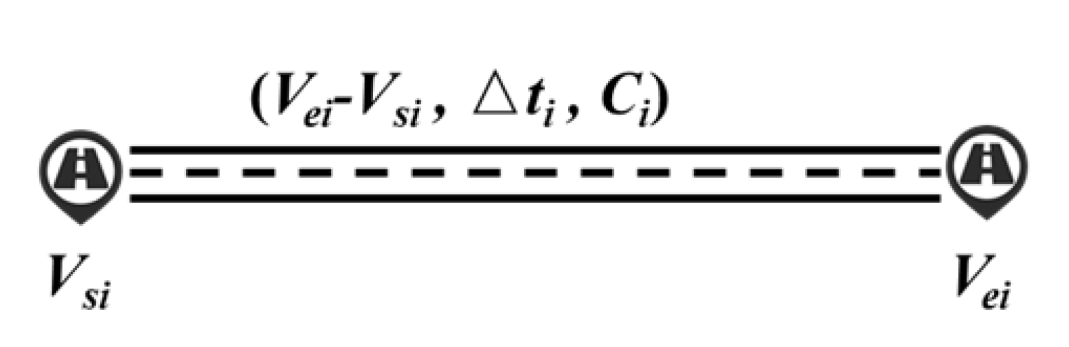
2.1. The Definition and Mathematical Model of DRTI

In order to obtain the optimal route, we must comprehensively consider the road congestion time, traffic flow, and road length. Thus, this paper defines a dynamic road traffic index (DRTI) as shown in Equation (1).

$$DRT{I}_i = \frac{(v_{ei}-v_{si}) \times (t_{ei}-t_{si})}{C_i}$$

(1)

Here, v_si represents the starting point of the i-th road, v_ei represents the ending point of the i-th road, t_ei represents the time to reach the ending point of the i-th road, t_si represents the time to start from the starting point of the i-th road, and C_i represents the traffic flow of the i-th road, i.e., the number of vehicles passing through the i-th road per minute. Obviously, C_i is an integer variable. The objective function (2) is given and should be minimized in order to obtain the optimal route scheme. Constraints (3)–(5) represent the topology constraint of the transportation network, congestion time constraint, and traffic flow constraint respectively.

$$\begin{array}{cc}min& {\displaystyle \sum _{i=1}^{n}DRT{I}_i = {\displaystyle \sum _{i=1}^n\frac{∆t_i(v_{ei}-v_{si})}{C_i}}}\end{array}$$

(2)

$$v\in \left\{v_1,v_2,v_3,\dots ,v_i\right\}$$

(3)

$$∆t_i \ge 0$$

(4)

$$C_i^{min} \le C_i \le C_i^{max}$$

(5)

It should be noted that the value of $∆t_i$ and $(v_{ei}-v_{si})$ can be obtained by some mature navigation software, such as Google Maps, Baidu Maps, etc. The traffic flow C_i can be predicted by a wavelet neural network, and the details are discussed in the next section. Thus, as shown in Figure 3, the dynamic characteristics of the transportation network can be described by these variables.

2.2. The Determination of Traffic Flow C_i

In this paper, a wavelet neural network (WNN) is used to predict the value of C_i. The WNN is developed from wavelet analysis theory. Combined with signal theory, wavelet has the following characteristics: it is a waveform with limited length, not an infinite waveform and from the point of numerical characteristics, the average value of a wavelet is zero and the DC component is zero too. The wavelet function is obtained from the basic mother wavelet function through translation transform and size compression. The time domain expression of wavelet transform is shown in Equation (6).

$$f_x(a,\tau ) = \frac{1}{\sqrt{a}}{\displaystyle {\int }_{-\infty }^{\infty }x(\omega )}\phi (a\omega )e^{j\omega }dt,a > 0$$

(6)

Here, $\phi (t)$ represents a basic wavelet function, the parameter $\tau$ refers to the size of translation transform, also named as translation factor; the parameter a represents the size of scale transform, also named as scale factor; and x(t) is the inner product function. From Equation (6), it can be seen that wavelet analysis can be used to analyze part of the signal; thus wavelet has a very good signal direction selectivity, and is widely used in the field of mathematics and physics. As shown in Figure 4, the structure of the WNN is the same as with that of the general neural network, such as BPNN. However, the difference is that the wavelet function with analytic form is selected as the activation function. According to the different practical application scenarios, the translation factor and scale factor of the wavelet function are adjusted to achieve the best training effect.

Assume that the training input set and the training output set are $x_i\in {\varphi }_x,y_i\in {\varphi }_y$ respectively. Then the mathematical expressions of the input layer, hidden layer, and output layer are respectively written as Equations (7)–(9).

$$u_i = x^T\cdot w(:,i)$$

(7)

$$h_i = \varphi (\frac{u_i-b_i}{a_i})$$

(8)

$$y_i = {\displaystyle \sum _{i=1}^m{c}_i}.h_i$$

(9)

Here, m is the number of hidden nodes, u_i and h_i are the input and output of the i-th node in a hidden layer respectively, and a, b and c are the structure parameters of the WNN respectively. According to the actual needs, the general optimization mathematical model of the WNN structure is written as shown in Equation (10).

$$minJ(w,a,b,c) = \frac{1}{N}{\displaystyle \sum _{n=1}^N{‖y_i-{\widehat{y}}_i‖}^2}+\lambda R(w,a,b,c)$$

(10)

Here, ${\widehat{y}}_i$ is the prediction output of the WNN’s output layer and R is the regular term constrained on the weight matrix W and C.

In this paper, a WNN is used to predict the traffic flow in the transportation network [21,22], and the time scale of prediction is 1 min. The WNN consists of three layers: input layer, hidden layer, and output layer. Part of the traffic flow data in the history database are used as training data, and the output layer outputs the predicted traffic flow data according to the trained model. Then, a detailed flow chart, as shown in Figure 5, is used to help the reader gain a better understanding. It should be noted that the WNN essentially adopts the gradient descent method; therefore, it may fall into the local optimal solution. Some valuable research has used PSO and GA algorithm to optimize the threshold selection of the WNN, which will not be discussed in detail here [23,24].

2.3. The Introduction of A-Star Algorithm

The traditional path determination algorithm includes the Dijkstra algorithm and the Warshall–Floyd algorithm. The Dijkstra algorithm is widely used to find the shortest route in complicated transportation networks. Its main feature is to extend from the starting point to the outside, layer by layer. Each time, it traverses the adjacent point of the nearest and inaccessible vertex from the starting point until it reaches the ending point. Obviously, the solving process of Dijkstra algorithm is complex and time consuming. It is a backward search algorithm in essence. When a subsequent node is added, the weight matrix of the transportation network stored in hardware needs to be calculated and updated again. For a real-time calculation of an urban transportation network with many nodes, it will be extremely time consuming and hardly realized as an online application.

The Warshall–Floyd algorithm is a dynamic programming algorithm used to find the shortest route between multisource points in the given weighted graph. Although the Floyd algorithm is easy to understand, it is also limited by computational complexity, and it is not suitable for an online computing complex network containing a large number of high-dimensional data.

In addition, the above two methods also have a common disadvantage: they can only deal with static transportation network information, only select the length of the line to establish the weight matrix, and ignore the complex traffic condition and dynamic characteristics, which are difficult to apply to the scene of an urban transportation network.

Thus, an A-Star (AS) algorithm is used to determine the optimal dynamic route in this paper, which avoids much repeated calculation and significantly improves the computational efficiency. The weight matrix a_ij used to depth search in the AS algorithm is constructed by DRTI, referred to in (1).

For the convenience of expression, this paper first makes the following definition:

• When the vertex i and vertex j coincide, the weight matrix a_ij can be expressed as Equation (11).

$$a_{ij} = 0$$

(11)

2.

When the vertex i and vertex j do not coincide and there are associated edges between them, the weight matrix a_ij can be expressed as Equation (12).

$$a_{ij} = \frac{\mathsf{∆}{t}_{ij}(v_j-v_i)}{C_{ij}}$$

(12)

3.

When the vertex i and j do not coincide and there is no associated edge between them, the weight matrix a_ij can be expressed as Equation (13).

$$a_{ij} = \infty$$

(13)

Similar to the Dijkstra algorithm, a priority queue is established in this paper, and we take the weight matrix a_ij between starting vertex and ending vertex as the priority, i.e., the optimal route is the route with the minimum value of a_ij. The priority of each vertex in an AS algorithm can be calculated by Equation (14). Here, P(i) is the comprehensive priority of vertex i, f(i) is the forward priority of vertex i, which represents the sum of weight a_ij between starting vertex and vertex i, and b(i) is the backward priority of vertex i, which represents the sum of weight a_ij between ending vertex and vertex i. Both f(i) and b(i) can be calculated by Equations (11)–(13).

$$P(i) = f(i) + b(i)$$

(14)

To gain a better understanding, a detailed flow chart of AS algorithm is given in

Table 2. The flow chart of AS algorithm to determinate optimal route.

Step 1	Initialize open set 1 and close set 2;
Step 2	Add starting vertex to the open set and set priority of starting vertex to 0, i.e., the highest priority;
Step 3	If the open set is not empty, select the vertex n with the highest priority in set;
Step 3.1	If vertex n is the ending vertex, the parent vertex is tracked gradually from the ending vertex n until it reaches the starting vertex;
Step 3.2	Return the found result route, and the algorithm ends;
Step 4	If vertex n is not the ending vertex, then remove vertex n from the open set and add it into the close set;
Step 4.1	Traverse all neighbor vertexes of vertex n;
Step 4.1.1	If the neighbor vertex m is in the close set, then skip vertex m and select the next neighbor vertex;
Step 4.1.2	If the neighbor vertex m is not in the open set, then set the parent vertex of vertex m as vertex n, calculate the priority of vertex m and add it into the open set;
Step 5	Repeat steps 2–4 until ending vertex is reached.

¹ The set including vertexes that have not been traversed is named open set; ² The set including vertexes that have been traversed is named close set.

.

3. The Optimal Installation Location of MEPS in a Power Grid

After the first stage that determines the optimal route in an urban transportation network, MEPSs can quickly reach the power grid. Then, determining the optimal installation location of a MEPS becomes an urgent problem to solve. There are several points that should be noted. The two steps mentioned in this paper are defined in a spatial dimension instead of a time dimension. The first step is that MEPS can go through the transportation network in the shortest time. Then, the second step is installing MEPSs. In terms of time dimension, the installation locations of MEPSs are determined by a control center after a fault occurs; this process can cost tens of seconds or several minutes. The emergency workers can obtain the MEPS allocation points before they reach the distribution network. Urban distribution networks contain many loads and the length of the transmission line is short; thus resistance of the transmission line cannot be ignored. Traditional power flow calculation methods, such as the Newton–Raphson method and the PQ decomposition method are no longer suitable for a distribution network, which will cause large errors. Therefore, this paper uses the forward–backward sweep method to calculate the power flow of the distribution network.

The forward–backward sweep method contains two steps of iterative calculation. First, take the feeder as the basic unit and calculate the power distribution from the ending node to the starting node section by section to obtain the injected power. Second, calculate the node voltage from the starting node to the ending node with the help of the obtained power distribution in the first step. The convergence criterion is whether the maximum value of voltage amplitude difference between two adjacent iterations is less than the allowable error. Equations (15) and (16) are the core of the forward–backward sweep method.

$$∆S_{ij}^k = \frac{{(P_j + P_{sum,j}^k)}^2 + {(Q_j + Q_{sum,j}^k)}^2}{{(V_j^k)}^2}(r_{ij} + j{x}_{ij})$$

(15)

$$S_{ij}^k = S_{sum,j}^k + S_j^k + ∆S_{ij}^k$$

(16)

Here, k represents iteration times, $∆S_{ij}^k$ represents power loss of branch connected nodes i and j; $P_j, Q_j, S_j^{}$ represent active power, reactive power, and load power of node j; $P_{sum,j}, Q_{sum,j}, S_{sum,j}^{}$ represent the sum of active power, reactive power, and load power of all branches which take node j as the starting node; $r_{ij}, x_{ij}$ represent the resistance and reactance of the branch connected nodes i and j; V_j represents the voltage of node j; S_ij represents the power from node i to node j.

It should be noted that in a distribution network, the ratio of resistance to reactance (R/X) is large. In order to improve the accuracy of calculation, the transverse component of voltage drop cannot be ignored. Thus, the accuracy voltage can be obtained by Equations (17)–(19).

$$∆V_{ij}^{k+1} = \frac{P_{ij}^k{r}_{ij} + Q_{ij}^k{x}_{ij}}{V_i^{k+1}}$$

(17)

$$\delta V_{ij}^{k+1} = \frac{P_{ij}^k{x}_{ij}-Q_{ij}^k{r}_{ij}}{V_i^{k+1}}$$

(18)

$$V_j^{k+1} = \sqrt{{(V_i^{k+1}-∆V_{ij}^{k+1})}^2 + {(\delta V_{ij}^{k+1})}^2}$$

(19)

Here, $∆V_{ij}^{k+1}, \delta V_{ij}^{k+1}$ represents the longitudinal and transverse component of voltage drop of branch connected nodes i and j; $P_{ij},Q_{ij}$ represent active power and reactive power from node i to node j, respectively. The model can be simplified if the backward–forward sweep method was used based on the ladder iterative technique. Detailed information can be seen from reference [25].

When extreme weather occurs in the distribution network, it will have an adverse impact on the stable power supply and power quality. In this paper, the optimal installing location of MEPS is determined by the objective to minimize the network loss under the premise of ensuring the power supply. The objective function and the corresponding constraints are expressed as (20)–(23), respectively. Among them, (21)–(23) represent voltage amplitude constraint, line current constraints, and power supply constraints, respectively. Here, g_i,j is the conductance of branches i to j. Equation (23) represents installation position constraint.

$$P_{loss} = min{\displaystyle \sum _{i=1,j=1,i\ne j}^{n_l}{g}_{i,j}[V_i^2+V_j^2-2V_i{V}_j\cos ({\theta }_i-{\theta }_j)]}$$

(20)

$$V^{min} \le V_i, V_j \le V^{max}$$

(21)

$$I \le I^{max}$$

(22)

$$L_{MEPS}\in \left\{n_1,n_2,n_3,n_4\dots ,n_i\right\}$$

(23)

4. Case Study

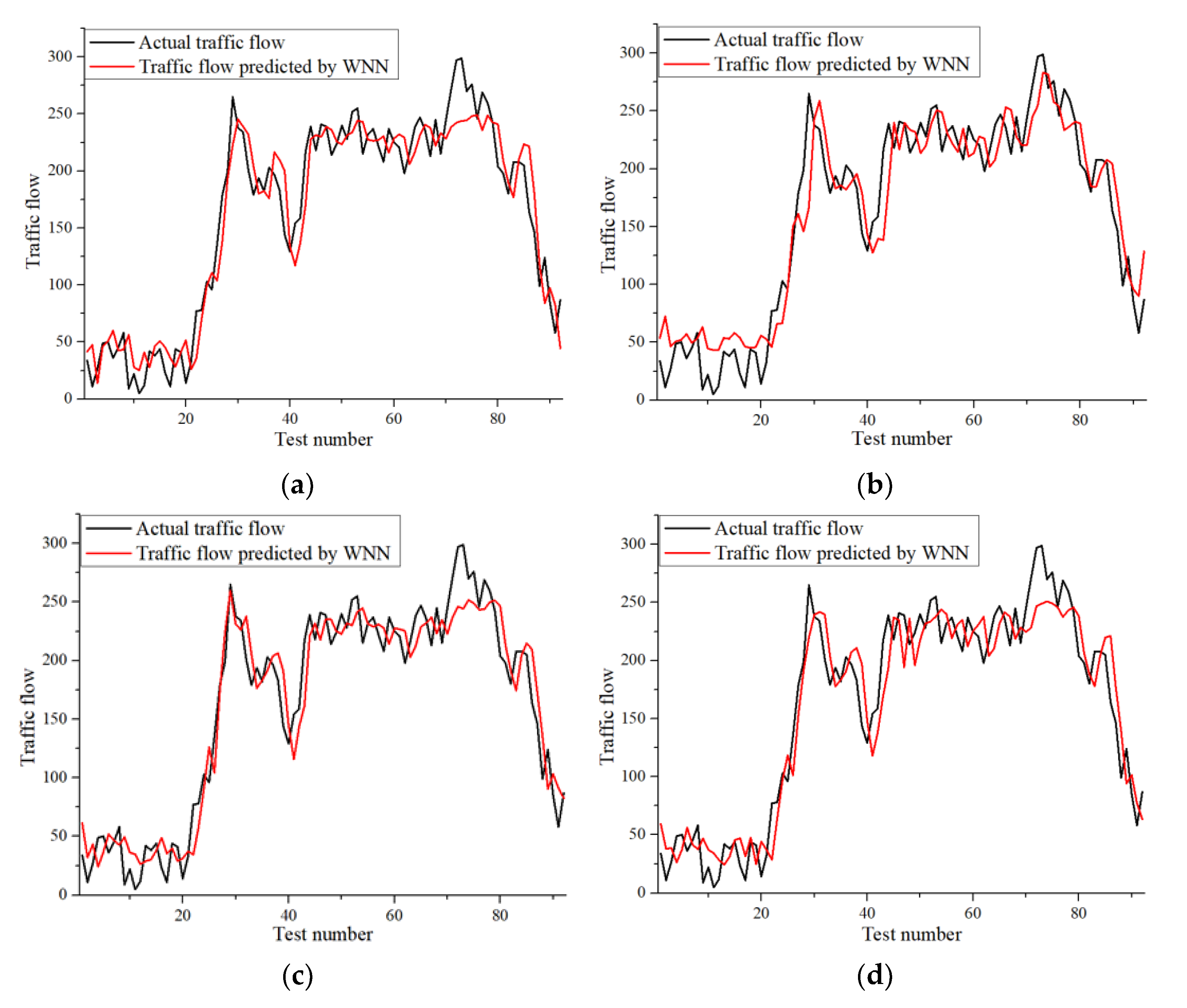
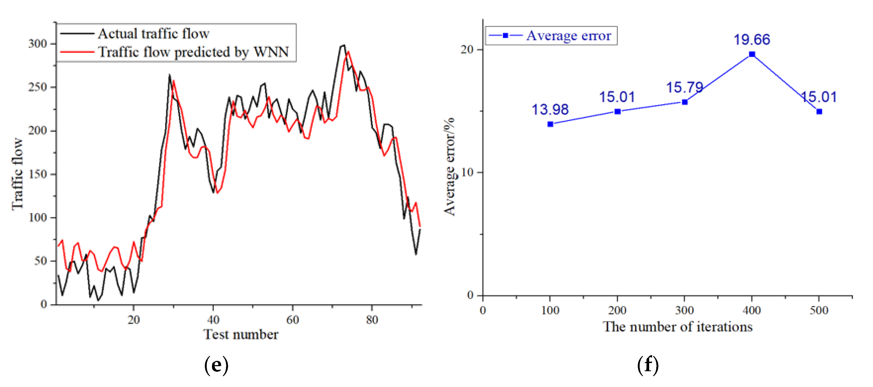
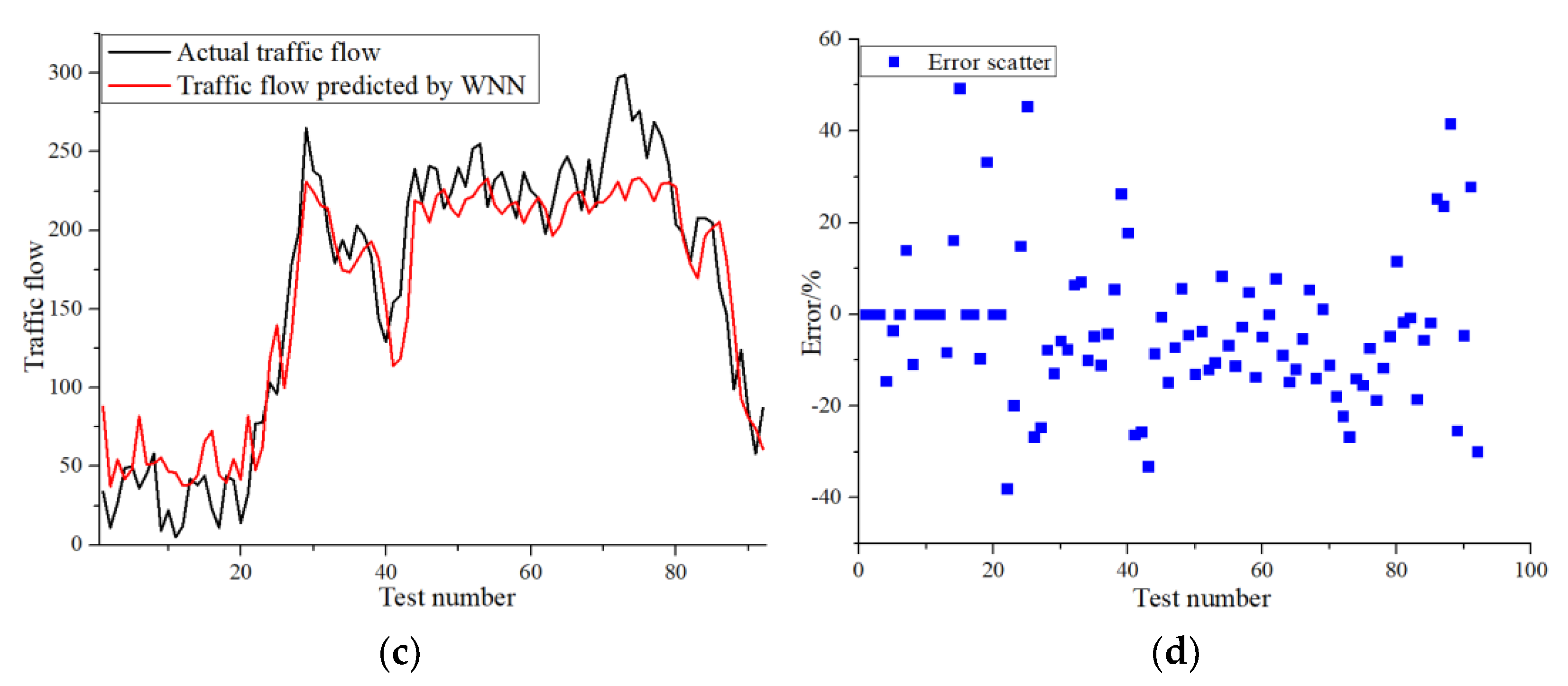
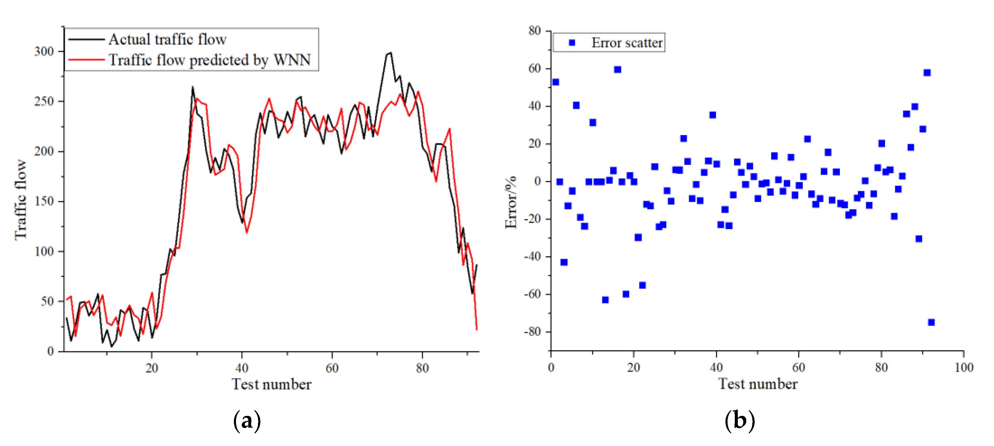
4.1. The Accuracy of WNN

In this paper, an WNN is used to predict traffic flow and the traffic flow data of an urban transportation network in China is used for training and testing. The parameters of the WNN are as follows: a total of 380 groups of traffic flow data are selected. Among them, 285 groups are selected as training samples, and the remaining 95 groups are used to test the performance of the network. The number of hidden layer nodes is 10 and the learning probability of the WNN is set to 0.1 and 0.01, respectively. Figure 6 shows the training output and average error analysis results of the WNN under different iteration times.

From the above results, it can be seen that the traffic flow predicted by the WNN is basically in line with the actual traffic flow, and the average error can be controlled below 15%, which can meet the needs of practical applications. When the iteration time is set to 100, the WNN can achieve the best results; when iteration times increase, the average error increases at the same time because the WNN essentially adopts the gradient descent method. That means that with the increasing of iteration times, it is possible to obtain the local optimal solution.

In addition, Scenario 1 and Scenario 2 are given to test the parameter sensitivity of the WNN. Detailed information of Scenario 1 and Scenario 2 is given below.

Scenario1: The number of hidden layer nodes is 10 and the learning probability of the WNN is set to 0.001 and 0.0001, respectively. Finally, the iteration time is set to 100.

Scenario 2: The number of hidden layer nodes is 10 and the learning probability of the WNN is set to 0.01 and 0.001, respectively. Finally, the iteration times are both set to 100.

From Figure 7, it can be seen that the predict output of the WNN remains unchanged under different scenarios in general. The error scatter mainly concentrated in the range of ±15%, which shows great performance of the WNN.

4.2. The Feasiblity of AS Algorithm

Three different transportation networks are used to illustrate the effectiveness and feasibility of an AS algorithm. The topology of the three transportation networks is shown in Figure 8. According to the expression method as shown in Figure 3, the dynamic characteristics of each route are shown in Figure 8. In order to reduce the complexity of the calculation, the original value of C_i is converted to the number of vehicles passing through the road per second. In the three transportation networks, the starting vertexes are 1, 1, 1 and the ending vertexes are 8, 8, 11, respectively.

Table 3. The time cost contrast among different transportation networks.

The Number of Transportation Networks	AS Algorithm		Dijkstra Algorithm		Warshall–Floyd Algorithm
	Calculation Results	Calculation Time	Calculation Results	Calculation Time	Calculation Results	Calculation Time
1	1, 3, 6, 8	0.0526 s	1, 2, 5, 8	1.2568 s	1, 2, 5, 8	1.6017 s
2	1, 3, 8	0.1486 s	1, 4, 7, 8	1.2362 s	1, 4, 7, 8	1.745 s
3	1, 2, 5, 9, 8, 11	1.357 s	1, 2, 5, 9, 6,7, 10, 11	3.4758 s	1, 2, 5, 9, 6,7, 10, 11	6.976 s

and

Table 4. The DRTI contrast among three different transportation networks.

The Number of Transportation Networks	AS Algorithm		Dijkstra Algorithm		Warshall–Floyd Algorithm
	Calculation Results	ΣDRTIi	Calculation Results	ΣDRTIi	Calculation Results	ΣDRTIi
1	1, 3, 6, 8	29.25	1, 2, 5, 8	38.667	1, 2, 5, 8	38.667
2	1, 3, 8	18.75	1, 4, 7, 8	37.5	1, 4, 7, 8	37.5
3	1, 2, 5, 9, 8, 11	31.83	1, 2, 5, 9, 6,7, 10, 11	50.83	1, 2, 5, 9, 6,7, 10, 11	50.83

show the results of the optimal route obtained by different methods and a comparison of computational efficiency. It can be seen from Table 3 that the AS algorithm adopted in this paper has the fastest computing speed, and the Warshall–Floyd algorithm has the slowest computing speed. This is because the AS algorithm avoids a large number of repeated calculations; thus improving the efficiency of the solution, which can meet the requirements of online computation. Table 4 shows the values of DRTI using different methods. Obviously, the DRTI value obtained by the AS algorithm is the smallest, that is, the route obtained by AS algorithm is optimal.

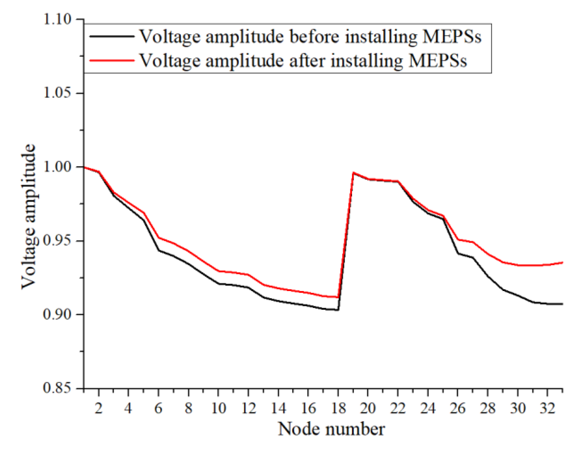
4.3. The Determination of the MEPS’s Location

In this section, an IEEE 33 test system is used to verify the effectiveness of the proposed method. The topology of the test system is shown in Figure 9. The case is tested on a laptop with 12G RAM and CPU Intel i5-7300HQ. This paper assumes that there are three MEPSs, and the capacity configurations of the three MEPSs are 100 kW + j40 kVar, 300 kW + j80 kVar, and 500 kW + j220 kVar. When the system is not installed with MEPSs, the forward–backward sweep algorithm is used to calculate the power flow of the distribution network and the voltage amplitude of each node, and the total active and reactive power loss of the system can be obtained. At this time, the active power loss of the system is 253.97 kW, and the reactive power loss is 169.03 kVar.

According to the calculation results, the optimal installation position of MEPSs is 18, 17, and 32, respectively. After the installation of MEPSs, the active power loss of the system is 185.68 kW, and the reactive power loss is 123.59 kVar. The active/reactive power loss of the system is significantly reduced, i.e., the power quality and economic performance of the system have been improved. Figure 10 shows the voltage amplitude comparison curve before and after installing MEPSs. It can be clearly seen that after the installation of MEPSs, the voltage amplitude of the system is higher than the original voltage amplitude, which improves the ability of the distribution network to cope with extreme weather.

In order to further verify the feasibility of the proposed method, another test system-IEEE 69 is adopted. The detailed information can be seen from the MATPOWER toolbox [26]. When the number of MEPSs in the system is three, the capacity configurations of the three MEPSs are 150 kW + j90 kVAR, 350 kW + j130 kVAR, and 550 kW + j270 kVAR. Before installing the MEPS in the distribution network, the active power loss and reactive power loss are 225 Kw and 100 kVAR, respectively. After installing the MEPS in the distribution network, the active power loss and reactive power loss are 125.6 Kw and 46.8 kVAR, respectively. Obviously, as shown in

Table 5. Analysis of energy loss before and after installing MEPS.

Test System		IEEE 33	IEEE 69
Energy loss before installing MEPS	Active power loss/Kw	253.97	225
	Reactive power loss/kVAR	169.03	100
Energy loss after installing MEPS	Active power loss/Kw	185.68	125.64
	Reactive power loss/kVAR	125.39	46.80

, the installation of a MEPS can effectively reduce network loss in a distribution system.

5. Conclusions

In this paper, a novel mobile emergency power source configuration scheme considering dynamic characteristics of a transportation network was presented. In the first stage, the optimal route can be determined in transportation network to meet the demand of real-time online application. In the second stage, with the help of the forward–backward sweep method, the optimal installation location of a MEPS can be obtained, and the power quality and economic benefits of the power grid can be improved significantly.

In future research, we will consider the extreme weather scenario generation and the uncertainty of modeling technology, and how to create the corresponding software application in the actual system as the core of our research.

References

1. Panteli, M.; Trakas, D.N.; Mancarella, P.; Hatziargyriou, N.D. Boosting the Power Grid Resilience to Extreme Weather Events Using Defensive Islanding. IEEE Trans. Smart Grid 2016, 7, 2913–2922. [Google Scholar] [CrossRef]
2. Dong, L.; Wang, C.; Li, M.; Sun, K.; Chen, T.; Sun, Y. User Decision-based Analysis of Urban Electric Vehicle Loads. CSEE J. Power Energy Syst. 2021, 7, 190–200. [Google Scholar]
3. Mohamed, M.A.; Chen, T.; Su, W.; Jin, T. Proactive Resilience of Power Systems Against Natural Disasters: A Literature Review. IEEE Access 2019, 7, 163778–163795. [Google Scholar] [CrossRef]
4. Pearson, J.; Wagner, T.; Delorit, J.; Schuldt, S. Meeting Temporary Facility Energy Demand with Climate-Optimized Off-Grid Energy Systems. IEEE Open Access J. Power Energy 2020, 7, 203–211. [Google Scholar] [CrossRef]
5. Yang, Y.; Tang, W.; Liu, Y.; Xin, Y.; Wu, Q. Quantitative Resilience Assessment for Power Transmission Systems Under Typhoon Weather. IEEE Access 2018, 6, 40747–40756. [Google Scholar] [CrossRef]
6. Ding, T.; Qu, M.; Wang, Z.; Chen, B.; Chen, C.; Shahidehpour, M. Power System Resilience Enhancement in Typhoons Using a Three-Stage Day-Ahead Unit Commitment. IEEE Trans. Smart Grid 2021, 12, 2153–2164. [Google Scholar] [CrossRef]
7. Liu, X. A Planning-Oriented Resilience Assessment Framework for Transmission Systems Under Typhoon Disasters. IEEE Trans. Smart Grid 2020, 11, 5431–5441. [Google Scholar] [CrossRef]
8. Liu, Y.; Li, J.; Wu, L. Coordinated Optimal Network Reconfiguration and Voltage Regulator/DER Control for Unbalanced Distribution Systems. IEEE Trans. Smart Grid 2019, 10, 2912–2922. [Google Scholar] [CrossRef]
9. Zheng, W.; Huang, W.; Hill, D.J.; Hou, Y. An Adaptive Distributionally Robust Model for Three-Phase Distribution Network Reconfiguration. IEEE Trans. Smart Grid 2021, 12, 1224–1237. [Google Scholar] [CrossRef]
10. Anagnostatos, S.D.; Halevidis, C.D.; Polykrati, A.D.; Koufakis, E.I.; Bourkas, P.D. High-Voltage Lines in Fire Environment. IEEE Trans. Power Deliv. 2011, 26, 2053–2054. [Google Scholar] [CrossRef]
11. Zhou, B.; Xu, D.; Li, C.; Cao, Y.; Chan, K.; Xu, Y.; Cao, M. Multi-objective Generation Portfolio of Hybrid Energy Generating Station for Mobile Emergency Power Supplies. IEEE Trans. Smart Grid 2018, 9, 5786–5797. [Google Scholar] [CrossRef]
12. Xu, Y.; Wang, Y.; He, J.; Su, M.; Ni, P. Resilience-Oriented Distribution System Restoration Considering Mobile Emergency Resource Dispatch in Transportation System. IEEE Access 2019, 7, 73899–73912. [Google Scholar] [CrossRef]
13. Lei, S.; Chen, C.; Zhou, H.; Hou, Y. Routing and Scheduling of Mobile Power Sources for Distribution System Resilience Enhancement. IEEE Trans. Smart Grid. 2019, 10, 5650–5662. [Google Scholar] [CrossRef]
14. Yang, Z.; Dehghanian, P.; Nazemi, M. Enhancing Seismic Resilience of Electric Power Distribution Systems with Mobile Power Sources. In Proceedings of the 2019 IEEE Industry Applications Society Annual Meeting, Baltimore, MD, USA, 29 September–3 October 2019; pp. 1–7. [Google Scholar]
15. Erenoğlu, A.K.; Erdinç, O.; Sancar, S.; Catalão, J.P.S. Post-Event Resiliency-Driven Strategy Dispatching Mobile Power Sources Considering Transportation System Constraints. In Proceedings of the 2021 8th International Conference on Electrical and Electronics Engineering (ICEEE), Antalya, Turkey, 9–11 April 2021; pp. 161–167. [Google Scholar]
16. Ye, H.; Chen, W.; Hu, Q.; Hao, W.; Wang, C.; Hou, K.; Jiang, X. A Voltage Control of Energy Storage Mobile Shelter Under Multi Energy Access. In Proceedings of the 2021 IEEE 4th International Electrical and Energy Conference (CIEEC), Wuhan, China, 28–30 May 2021; pp. 1–6. [Google Scholar]
17. Erenoğlu, A.K.; Erdinç, O. Post-Event restoration strategy for coupled distribution-transportation system utilizing spatiotemporal flexibility of mobile emergency generator and mobile energy storage system. Electr. Power Syst. Res. 2021, 199, 378–386. [Google Scholar] [CrossRef]
18. Wang, Y.; Xu, Y.; Li, J.; He, J.; Liu, J.; Zhang, Q. Dynamic load restoration considering the interdependencies between power distribution systems and urban transportation systems. CSEE J. Power Energy Syst. 2020, 6, 772–781. [Google Scholar]
19. Zhu, S.; Hou, H.; Zhu, L.; Liang, Y.; Wei, R.; Huang, Y.; Zhang, Y. An optimization model of power emergency repair path under typhoon disaster. Energy Rep. 2021, 7, 204–209. [Google Scholar] [CrossRef]
20. Sedgh, S.A.; Doostizadeh, M.; Aminifar, F.; Shahidehpour, M. Resilient-enhancing critical load restoration using mobile power sources with incomplete information. Sustain. Energy Grids Netw. 2021, 26, 104–113. [Google Scholar]
21. Khan, M.A.; Uddin, M.N.; Rahman, M.A. A Novel Wavelet-Neural-Network-Based Robust Controller for IPM Motor Drives. IEEE Trans. Ind. Appl. 2013, 49, 2341–2351. [Google Scholar] [CrossRef]
22. Shi, B.; Xu, L.; Meng, W. Applying a WNN-HMM Based Driver Model in Human Driver Simulation: Method and Test. IEEE Trans. Intell. Transp. Syst. 2018, 19, 3431–3438. [Google Scholar] [CrossRef]
23. Song, Y.; Chen, Z.; Yuan, Z. New Chaotic PSO-Based Neural Network Predictive Control for Nonlinear Process. IEEE Trans. Neural Netw. 2007, 18, 595–601. [Google Scholar] [CrossRef] [PubMed]
24. Liu, J.; Huang, J.; Sun, R.; Yu, H.; Xiao, R. Data Fusion for Multi-Source Sensors Using GA-PSO-BP Neural Network. IEEE Trans. Intell. Transp. Syst. 2021, 22, 6583–6598. [Google Scholar] [CrossRef]
25. Marchesan, A.C.; Marconato, G.V.; Costa, L.M.A.; Gallas, M.R.; Ferri, C.B.; Cardoso, G. Performance analysis of forward/backward sweep power flow methods for radial distribution systems. In Proceedings of the 2018 Simposio Brasileiro de Sistemas Eletricos (SBSE), Niteroi, Brazil, 12–16 May 2018; pp. 1–6. [Google Scholar]
26. Zimmerman, R.D.; Murillo-Sánchez, C.E.; Thomas, R.J. MATPOWER: Steady-State Operations, Planning, and Analysis Tools for Power Systems Research and Education. IEEE Trans. Power Syst. 2011, 26, 12–19. [Google Scholar] [CrossRef] [Green Version]
Figure 1. MEPS in China National Grid Corporation.
Processes 09 01935 g001
Figure 2. Diagram of MEPS configuration scheme.
Processes 09 01935 g002
Figure 3. The expression of the transportation network’s dynamic characteristics.
Processes 09 01935 g003
Figure 4. The structure of the WNN.
Processes 09 01935 g004
Figure 5. The structure of the WNN flow chart of traffic flow prediction using the WNN model.
Processes 09 01935 g005
Figure 6. The predict output of the WNN and average error analysis. (a) Iteration times = 100; (b) Iteration times = 200; (c) Iteration times = 300; (d) Iteration times = 400; (e) Iteration times = 500; (f) Average error analysis.
Processes 09 01935 g006aProcesses 09 01935 g006b
Figure 7. The predict output of different scenarios and error scatter. (a) The output of Scenario 1; (b) Error scatter of Scenario 1; (c) The output of Scenario 2; (d) Error scatter of Scenario 2.
Processes 09 01935 g007aProcesses 09 01935 g007b
Figure 8. The topology of three different transportation networks. (a) Transportation network 1; (b) Transportation network 2; (c) Transportation network 3.
Processes 09 01935 g008
Figure 9. The topology of an IEEE 33 test system.
Processes 09 01935 g009
Figure 10. The voltage amplitude comparison curve before and after installing MEPSs.
Processes 09 01935 g010