Article

A Multi-Scale Model for the Spread of HIV in a Population Considering the Immune Status of People

by
Sol de Amor Vásquez-Quintero
1,
Hernán Darío Toro-Zapata
1,* and
Dennis Alexánder Prieto-Medellín
2
1
Licenciatura en Matemáticas, Universidad del Quindío, Quindío 630004, Colombia
2
Gerontología, Universidad del Quindío, Quindío 630004, Colombia
*
Author to whom correspondence should be addressed.
Processes 2021, 9(11), 1924; https://doi.org/10.3390/pr9111924
Submission received: 10 April 2021 / Revised: 11 October 2021 / Accepted: 20 October 2021 / Published: 27 October 2021
(This article belongs to the Section Biological Processes and Systems)

Abstract

:
A multi-scale mathematical model is proposed, seeking to describe the propagation of Human Immunodeficiency Virus (HIV) in a group of young people between 15 and 24 years of age, through unprotected sexual contact. The uses of antiretroviral therapy (ART) and therapeutic failure are considered to show how the rate of propagation and prevalence are affected. The model consists of a complex network modeling the interactions on the population scale, coupled with the immunological dynamics of each individual, which is modeled by a system of differential equations. The immunological model allows to observe some known facts from the literature, such as to control HIV infection in the immune system, it is necessary to reduce the probability of healthy CD4 T cells becoming infected or increase the probability at which cells of the specific cell response against HIV eliminate infected CD4 T cells. At the population level, it is shown that, to have a high prevalence, it is not necessary for the virus to spread rapidly at the beginning of the simulation time. Additionally, it is observed that a greater number of sexual partners induces higher HIV prevalence. Using ART in the immune system reduces the number of infected CD4 T cells and, consequently, helps to reduce the spread of infection at the population scale. An important result observed in simulations is that the average number of HIV carriers who abandon ART is greater than those who access it. The study adds to the available literature an original simulation model that describes the dynamics of HIV propagation in a population, considering the immune state of people within that population, and serves as a basis for future research involving more detailed aspects aiming for a model closest to reality.

1. Introduction

The Human Immunodeficiency Virus (HIV) has managed to propagate and remain in the human population for decades; it is one of the most serious public health problems globally, having no cure and each year taking new lives when the infection goes on to become an acquired immunodeficiency syndrome (AIDS) [1,2]. Additionally, over time, not only does it increase the number of infected people, but it increases the number of new infections every year [3].
The HIV attacks the immune system of the infected person, specifically, attacking and destroying the CD4 T lymphocytes, which are a type of cell in charge of the fabrication of antibodies to combat infections caused by external agents [4]. Once the virus enters the person’s body, it is recognized by the body’s defense system and starts the infection process. First, it adheres to healthy CD4 T cells, then, the virus introduces its genetic material and viral components into the cell nucleus that then begins replication (after immunological activation) of the virus within it, goes into the bloodstream, and starts propagating throughout the body until infecting other healthy CD4 T cells [5].
One of the populations most vulnerable to acquire the virus are young people between 15 and 24 years of age; different studies reveal that it is in this stage when they start an active sex life, may have a greater number of sex partners, engage in unprotected sexual intercourse, and incur in the use of drugs and alcohol that are scenarios of increased risk; furthermore, many young people ignore how HIV is transmitted and most fear being tested to know their serological status [6,7,8]. This is how one third of new infections occurs in this age range globally [9] and in Colombia, for 2019, 24.8 % of those infected were young people [10]. This is why it is fundamental to conduct research that contributes to studying the epidemic, taking this age group as the object of study.
Antiretroviral therapy (ART) consists of the combination of three or more medications that help to maintain low levels of viral load, stable levels of healthy CD4 T cells, and diminish the probability of infecting other people [11]. In 2020, of the 37.7 million people who lived with HIV worldwide, 27.5 million had access to ART, that is, 73.3 % of those infected [3]. Unfortunately, not everyone manages to have access to ART, primartly because they do not know their serological status; more so, many reasons cause people, in spite of using ART, to abandon it; among the known factors, there are the high costs of medications, side effects, and not adhering to therapy [12]. By early 2020, in eastern and southern Africa, of the 20.7 million people living with HIV, 15 million had access to ART; in Asia and the Pacific, there were an estimated 5.8 million people with HIV of which 3.5 million had access to treatment; in West and Central Africa, there were 4.9 million people with HIV and only 2.9 million had access to ART; in Latin America, the number of HIV infected was 2.1 million and only 1.3 million had access to ART; on the other hand, in the Caribbean there were 330,000 people infected with HIV and 210,000 of them had access to ART. Additionally, in the Middle East and North Africa, there were 240,000 people who had HIV and only 92,000 used ART; in Eastern Europe and Central Asia as well, the figures were alarming, given that of the 1.7 million people living with HIV, only 730,000 had access to treatment. Finally, it is worth mentioning the cases of western and Central Europe, and North America, where 2.2 million people had HIV and 1.8 million people had access to treatment [3]. Therefore, in a population model for the spread and control of HIV infection, it is convenient to consider access and adherence to ART [3].
Prior research has sought to understand the behavior of the virus in the immunological and/or population scale. This is the case of [13] that studies the dynamics of infection by HIV through stochastic birth and death processes and from the systems of differential equations that represent a real system. Additionally, ref. [14] shows the behavior of the virus in a population of susceptible people, people infected without ART, and people infected with ART; they propose a mathematical model based on ordinary differential equations that interprets the effect of effective access and therapeutic failure have on said populations. Finally, a study that elaborates a mathematical model for the dynamics of HIV transmission centered on the functions of the immune response cells, and considering active and inactive cytotoxic immune cells, was conducted in [14], which evaluates two different scenarios of the infection (early stage and advanced stage) and employs the optimal control theory.
During the last two decades, there has been an increase in the study and use of complex networks in different contexts [15,16,17,18,19,20,21,22]; particularly, complex networks have gained strength when representing sexual contacts among people. We, herein, introduce a model that uses complex networks to study the dynamics of HIV propagation in people between 15 and 24 years of age, who interact through sexual contacts, considering at the same time the dynamics of infection in the immune system of each young person; the immune system is modeled through the system of ordinary differential Equations (ODE) proposed in [23]. The research gains importance by being a multi-scale model that integrates two components: the population (network) and the immunological (ODE system) because the population dynamics cannot be detached from the immunological, thus, adding to previous research that studies both components separately.
The study permits obtaining some standard results that essentially validate the model, for example, that the infection is controlled when reducing the values of the probability of healthy CD4 T cells becoming infected and increasing the probability of active cytotoxic cells of eliminating infected CD4 T cells. In addition, when using reverse transcriptase inhibitors (RTI) and protease inhibitors (PI), the rate of virus propagation is reduced and the infection is also controlled in the immune system, obtaining better results when these medications are used in combination. Moreover, it is shown that the greater the number of sex partners a person has, the greater the prevalence of the virus within the population and the infection will propagate at higher rates, as long as the sexual encounters take place unprotected. A result that is not trivial at all is that, to have a population with high prevalence of HIV carriers, it is not necessary for the virus to propagate rapidly at the beginning of the propagation process. It is observed in all the network simulations performed that the number of HIV carriers without ART was higher than the number of HIV carriers with ART, which indicates a higher number of HIV carriers who abandon ART than those who have access to it.
This paper is carried out in the following manner: Section 2 describes the population model (the sexual contact network) and presents the immunological model. Section 3 conducts the respective local stability analysis of the immunological model, discussing the invariance region, equilibrium points, and the basic reproduction number. The local stability is illustrated through simulations performed for the immunological model, varying the different parameters; then, the coupling algorithm of the immunological and population scales is formulated. Finally, simulations are performed of the coupled model. Section 4 exposes the conclusions obtained and, in the end, the references used are shown.

2. Materials and Methods

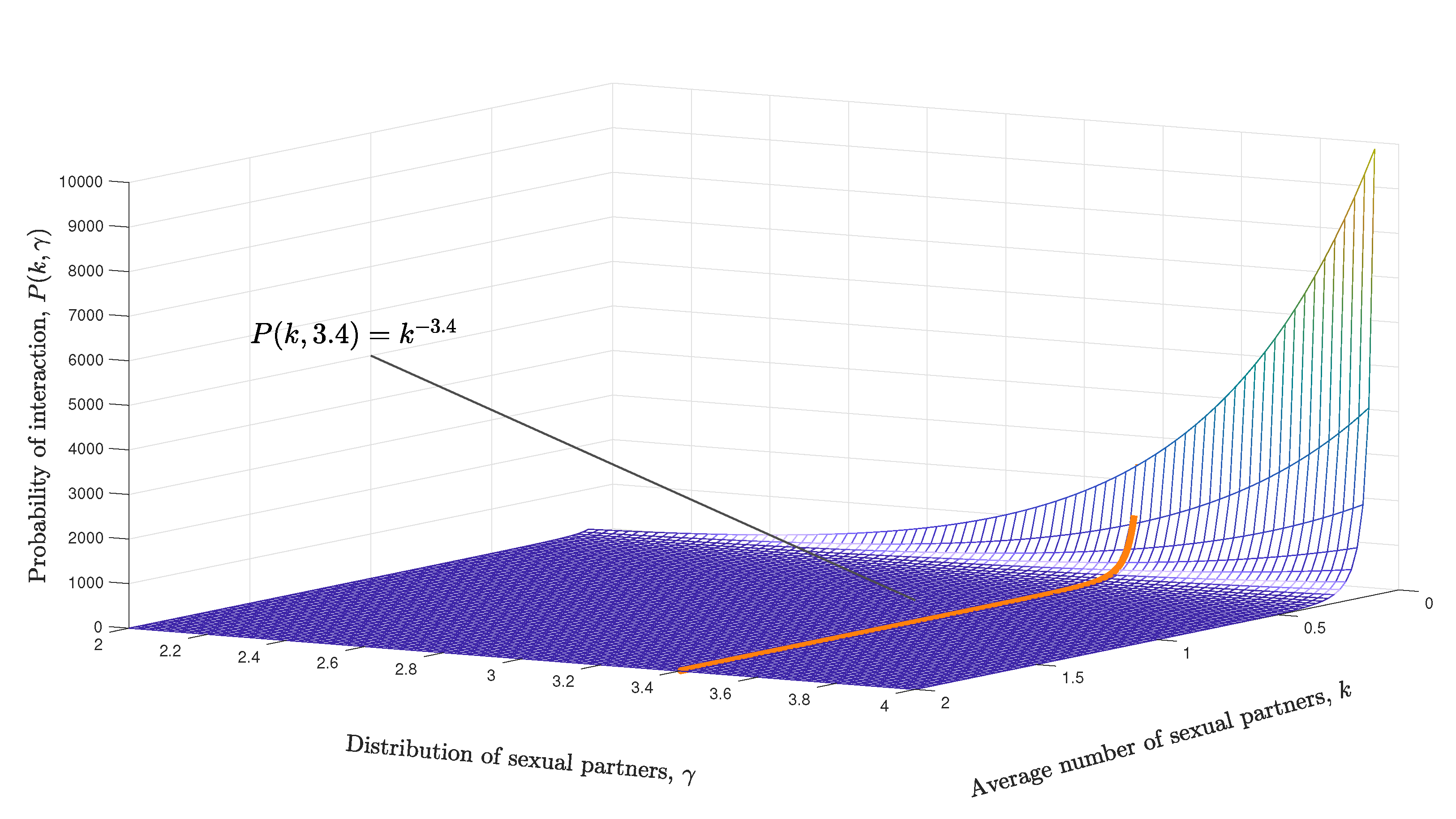
2.1. Population Model: Sexual Contact Network

The study population are young people between 15 and 24 years of age and is modeled through a complex network, where the vertices represent people and the edges are the potential unprotected sexual encounters with each other, through which the virus can propagate. No differentiation is made regarding gender, sexual orientation; nor does the study consider the use of stimulants, like hallucinogenic drugs or alcohol. The model considers a constant and finite population N T ; hence, it does not take into account new young people entering the network, nor their deaths. A cluster scale-free network is generated (according to the Barabási–Albert model, being scale-free means that there is no preferred scale or preferred number of edges for each vertex with respect to the rest [15]), in which the probability P ( k , γ ) of a vertex in the network interacting with other vertices decays through a power law P k γ [15], where k is the average number of sexual partners and γ is related to the partners’ distribution, it is a parameter whose value depends on the specific type of network; more precisely, γ modulates the probability P, given that for values greater than γ , P decreases faster [24,25]. In addition, the network is random non-directed and uses the algorithm by Holm and Kim [24]. It is noteworthy that it is considered a complex scale-free network cluster type because it best adjusts to the phenomena that occur in nature, also due to its high heterogeneity, which means that nodes exist with very few connections, moderately connected nodes, and extremely connected nodes. It is not considered a small world model because it is a homogeneous network in which all nodes have approximately the same number of links, and what is sought is to achieve a somehow more realistic situation; therefore, it must be considered that there will be people in our population with a greater number of sexual partners than others [25,26,27,28].
Figure 1 shows the plot of P in the ( k , γ , P ) -space, where the orange curve corresponds to the fixed value γ = 3.4 used in the simulations in this study. Figure 1 shows how the probability P diminishes as the average number of sexual partners increases; also, at a low average number of sexual partners and high values in the distribution of said partners, the probability of a vertex from the network to interact with others will be higher.
Use of ART is taken into account, considering that for a person to have access to it, they must first be tested, diagnosed as a carrier, and have the economic resources (their own or from health insurance) to acquire the medications. The model includes non-adherence to therapy that can be caused by consumption of psychoactive substances, depression, low level of schooling, low levels of trust in the benefits of ART, greater number of tablets and dosage, lack of family and/or social support, etc. [29], and considers therapeutic failure, which has drug resistance, drug toxicity (degree of adverse effects), and non-observance of ART as principal causes [30].
The study comprised a population of N T young people between 15 and 24 years of age, where x i = x i ( τ ) , y i = y i ( τ ) , and z i = z i ( τ ) are the number of young people susceptible of acquiring the virus, young carriers of the virus who use ART, and young carriers who do not use ART, respectively, where τ is the discrete simulation time and we define t f as the final simulation time, thus, τ = 0 , , t f . Finally, x i = 1 , , m , y i = 1 , , n and z i = 1 , , l , then the relation m + n + l = N T holds for every τ since the population is assumed constant over time, an oversimplification that can be relaxed in future work.
The complex network is defined by the { G , Γ } pair, where G is a graph, that is, an ordered pair of disjointed sets V , A that correspond to the set of vertices V and edges A, and Γ an evolution operator that determines changes of the network [18]; that is,
V , A τ + 1 = Γ V , A τ V , A 0 = V 0 , A 0 , τ = 0 , , t f ,
where V 0 , A 0 is the initial configuration of vertices and edges of the network at τ = 0 . Additionally, the configuration V , A over time τ + 1 is given by the Γ operator applied in the previous iteration τ , thus originating a “sequence” of networks that correspond to iterations over time. The evolution operator Γ , governing the network changes, implicitly considers two fundamental aspects:
1.
Infection dynamics by the virus in the immunological scale.
2.
Defines the virus propagation in the population scale, considering aspects from the immunological scale.
The coupling of both dynamics takes place aiming to achieve a somewhat more realistic model where the events in the population scale are affected by the state of the infection in the immune system of each infected individual in the population. The parameters and variables considered to define changes in the network are effective use and abandonment of ART, average viral load, and number of healthy CD4 T cells of each infected person (details of the coupling algorithm are described in the Results section). Table 1 shows the parameters used in the population model with their respective values used in simulations.

2.2. Model for HIV Infection in the Immunological Scale

A mathematical model that considers the dynamics of the HIV infection while using ART has been described in [23], which will be used in this work. The following describes the model and the Appendix A contain proofs for the local stability analysis. Use of ART seeks to reduce the number of new infected cells through RTI and PI, which are denoted, respectively, by u 1 and u 2 , such that u i ∈ [0, 1] for i = 1 , 2 . When u i = 1 , it means that use of medication was efficient by 100% and u i = 0 represents a 0% efficiency or absence of ART.
In the first place, T = T ( t ) is the average number of healthy CD4 T cells in a time t, these cells are produced at a constant rate σ in the organism and their natural death is described by the rate μ , so that μ T represents the average of healthy CD4 T dying naturally. The CD4 T cells are infected upon contact with the viral particles V = V ( t ) over time, at a probability β . The mass-action principle permits establishing that the average of new infected cells is proportional to the product of healthy CD4 T cells with the infectious viral particles [13]; this permits the assumption that the average number of cells that become infected is β ( 1 u 1 ) T V , where ( 1 u 1 ) is the failure rate of RTI. The equation to describe the variation of healthy CD4 T cells with respect to time t is:
T ˙ = σ β ( 1 u 1 ) T V μ T
where the dot denotes time derivative. The average number of infected cells over time is denoted T * = T * ( t ) ; which die at a rate δ ; thus, δ T * is the average number of infected cells that die due to causes associated with the virus. This death is known as cellular lysis, consisting in the rupture of the cell membrane. The differential equation that describes the variation of infected CD4 T cells is:
T * ˙ = β ( 1 u 1 ) T V γ T * M * δ T *
To explain the term γ T * M * , consider that T * cells stimulate the specific cell immune response against HIV (CD8 T cells) that are inactive M = M ( t ) and become active M * = M * ( t ) . The CD8 T cells recognize and destroy only the infected cells through direct attack, injecting toxic enzymes that cause their destruction [30,31]. Thus, M is the average number of CD8 T immune cells inactive at a given time t and M * represents the average number of activated CD8 T immune cells at a given time t. The M * cells are in charge of destroying the T * cells with a probability γ , then γ T * M * , through the mass-action principle, is the average number of infected cells destroyed by the specific cell immune response. The CD8 T cells are produced in the organism at a constant rate λ and the average of cells dying naturally is described by ρ M , where ρ is the death rate of the CD8 T cells. It is assumed that the influence of the T * cells stimulates the active immune response M * , according to the mass-action principle at a probability ψ , hence, the average number of inactive M cells that activate against HIV is given by ψ T * M . Thus, the equation for the average number of M cells remains:
M ˙ = λ ψ T * M ρ M
Furthermore, it is considered that proliferation of activated CD8 T cells at a probability α stimulated by the presence of infected cells T * ; then, through the mass-action principle, α T * M * represents the average of new active CD8 T cells produced through proliferation. Finally, it is considered that cells from the active cell response M * die at a rate ρ , thus, ρ M * is the average of M * cells dying naturally. Due to the aforementioned, the differential equation is:
M * ˙ = α T * M * + ψ T * M ρ M *
When the T * cells die due to cellular lysis, their cell membranes rupture, release intracellular material and a large amount of new infectious and non-infectious virions (the latter as long as the PI are used); recall V = V ( t ) is the average number of infectious viral particles in a time t and denote W = W ( t ) the average number of non-infectious viral particles at a given time t. The elimination rate of viral particles is represented with c; hence, c V and c W represent the average number of infectious and non-infectious viral particles eliminated, respectively. In the model, replication of V and W is described through N δ T * in which N is the average number of viral particles produced by an infected T * cell and the production of non-infectious virions depends on the use of PI (with effectiveness u 2 ). Therefore, expressions N δ ( 1 u 2 ) T * and N δ u 2 T * represent the average number of infectious and non-infectious virions, respectively, produced by each infected cell, bearing in mind the effect of ART. The differential equations that describe this behavior are:
V ˙ = N δ ( 1 u 2 ) T * c V
and
W ˙ = N δ u 2 T * c W
With the assumptions described, the system modelling HIV replication in an infected person’s organism, considering ART, is given by the system (7) of differential equations. Table 2 describes the parameters used in the immunological model.
T ˙ = σ β ( 1 u 1 ) T V μ T T * ˙ = β ( 1 u 1 ) T V γ T * M * δ T * M ˙ = λ ψ T * M ρ M M * ˙ = α T * M * + ψ T * M ρ M * V ˙ = N δ ( 1 u 2 ) T * c V W ˙ = N δ u 2 T * c W
The model (7) was proposed in [23], but its local stability was not analyzed with control; here, we perform this analysis and use it to describe the immune system of each person in the complex network.

3. Results

3.1. Local Stability Analysis of the Immunological Model

The model (7) is defined in an invariance region whose importance is to guarantee that the populations do not become negative or grow indefinitely; in other words, it guarantees that the model’s solutions make biological sense. Mathematically, the region is a compact set that finally ( t 0 ) will contain the system’s solutions, that is, ensuring that the system’s solutions (7) enter the region and remain in it for all t 0 . The demonstration of the Proposition 1 is found in the Appendix A.
Proposition 1.
If γ α , the system (7) is defined in the positively invariant region Ω = x R 6 | 0 T σ μ , 0 G σ + λ ε , 0 D N δ ( σ + λ ) ε c , where x = ( T , T * , M , M * , V , W ) ; G = T + T * + M + M * and D = V + W .
Condition γ α means that the probability of the active CD8 T cells of eliminating the infected CD4 T cells being higher than the probability of replicating the active CD8 T cells.
The stationary solutions or equilibrium points represent the values of variables T, T * , M, M * , V, and W where there is no change in the system’s behavior; that is, they are constant solutions E ¯ = T ¯ , T ¯ * , M ¯ , M ¯ * , V ¯ , W ¯ of system (7) whose coordinates are:
T ¯ = σ c N δ β ( 1 u 1 ) ( 1 u 2 ) T ¯ * + c μ , M ¯ = λ ψ T ¯ * + p , M ¯ * = λ ψ T ¯ * ( ψ T ¯ * + ρ ) ( ρ α T ¯ * ) , V ¯ = N δ ( 1 u 2 ) T ¯ * c , W ¯ = N δ u 2 T ¯ * c .
From (8) for T ¯ * = 0 , the virus free equilibrium E ¯ 0 =   σ μ , 0 , λ ρ , 0 , 0 , 0 is obtained, where σ μ represents the average number of healthy cells T and λ ρ represents the average number of inactive CD8 T cells. On the other hand, to have equilibria in presence of virus, note that it is required ρ > α T ¯ * to have a non-negative M ¯ * . In (8), we denote T ¯ * the solution of the cubic equation:
A ξ 3 + B ξ 2 + C ξ + D = 0 ,
where,
A = δ α ψ F , B = γ λ ψ F + δ F ρ ( α ψ ) + δ α ψ c μ α ψ σ F , C = δ ρ 2 F c μ γ λ ψ + δ ρ c μ ( α ψ ) + F ρ σ ( ψ α ) , D = δ ρ 2 c μ + σ ρ 2 F ,
and F = N δ β ( 1 u 1 ) ( 1 u 2 ) . To study the system’s behavior in presence of viremia through a stability analysis of (7), it is convenient to find the basic reproduction number R 0 , a number that has been widely studied in the spread of epidemics on a population scale, and whose definition is also applicable in this type of models on an immunological scale, indeed, it corresponds to the average number of secondary cells infected in a susceptible cellular population by an infected cell with certain initial viral load [13,34,35]. Mathematically, R 0 is the spectral radius of the next-generation matrix evaluated in the virus-free equilibrium [36] (see Appendix A). For system (7), it is given explicitly by:
R 0 = N β ( 1 u 1 ) ( 1 u 2 ) c σ μ .
The R 0 is important because, theoretically, it determines if there will be a peak in viral replication ( R 0 > 1 ) and, on the contrary, there will be no increase in the viral load when R 0 < 1 , which means that the infection is not established and manages to “disappear”, as established in the following results. In particular, the analysis of local stability of the virus-free equilibrium E ¯ 0 permits determining conditions for the system’s solutions to stabilize close to such values or approach them over time, i.e., determine “theoretical” conditions under which the infection does not manage to establish in the immune system.
Proposition 2.
The virus-free equilibrium E ¯ 0 = σ μ , 0 , λ ρ , 0 , 0 , 0 is locally asymptotically stable if and only if R 0 < 1 .
This means that if a person is susceptible of acquiring HIV, but satisfies R 0 < 1 , then the infection “theoretically” is not established in the immune system, and the initial viral load becomes undetectable; this result is theoretical, given that HIV infection has no cure [34,35,37]. The demonstration of the Proposition 2 is found in the Appendix A.
Proposition 3.
If R 0 > 1 , there is a single equilibrium in presence of viremia given by E ¯ 1 = T ¯ , T ¯ * , M ¯ , M ¯ * , V ¯ , W ¯ .
By the nature of the system, it is expected the equilibrium in presence of viremia E ¯ 1 to be locally asymptotically stable when R 0 > 1 (in that case, as already proven by Proposition 2, the virus-free equilibrium is unstable), since it was not possible to perform the analytical proof (due to the algebraic difficulty), this remains a conjectured result. Appendix A presents the demonstration of Proposition 3 and the conjecture will be illustrated numerically via simulation. However, the stability of the equilibrium in the presence of viremia implies the occurrence of infection peaks in the organism and the variation in time of the cellular levels and the viral loads. Usually, the system’s transient describes oscillations before reaching the stability values, which will be illustrated in the next subsection.

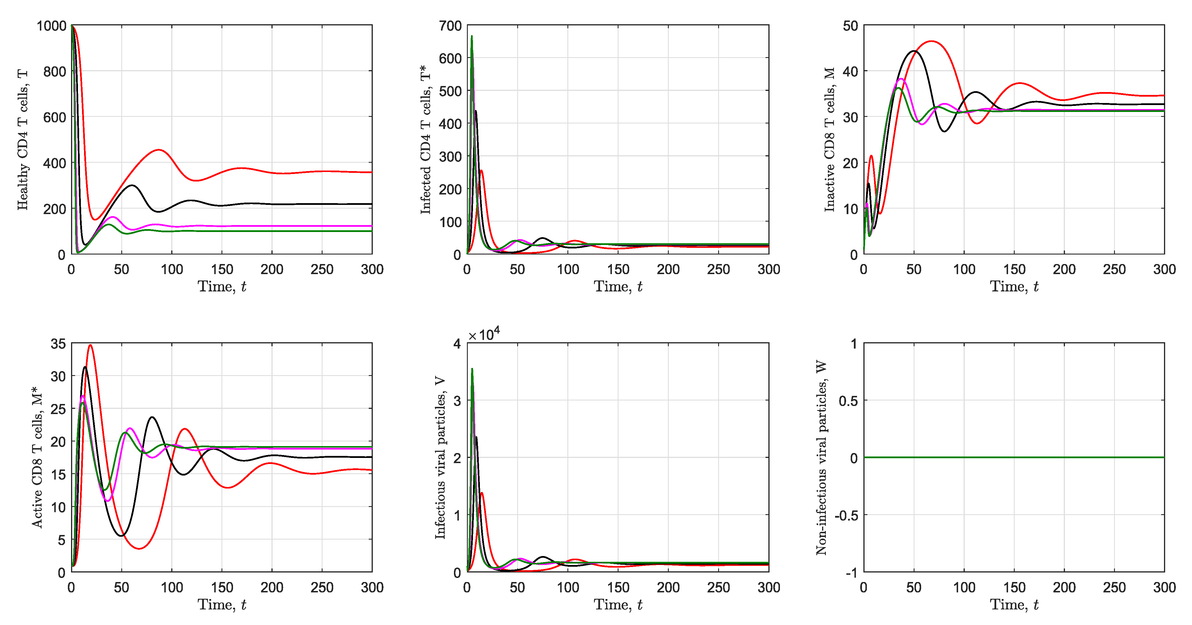
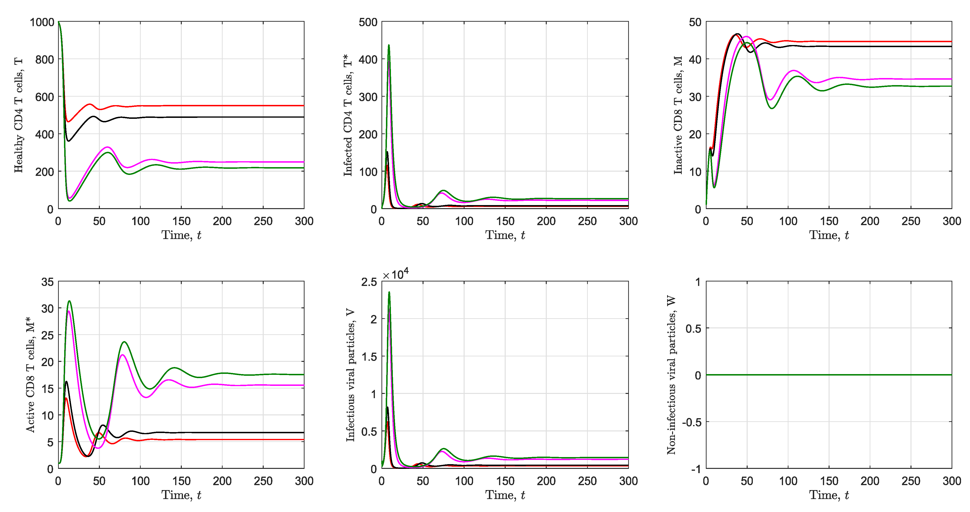
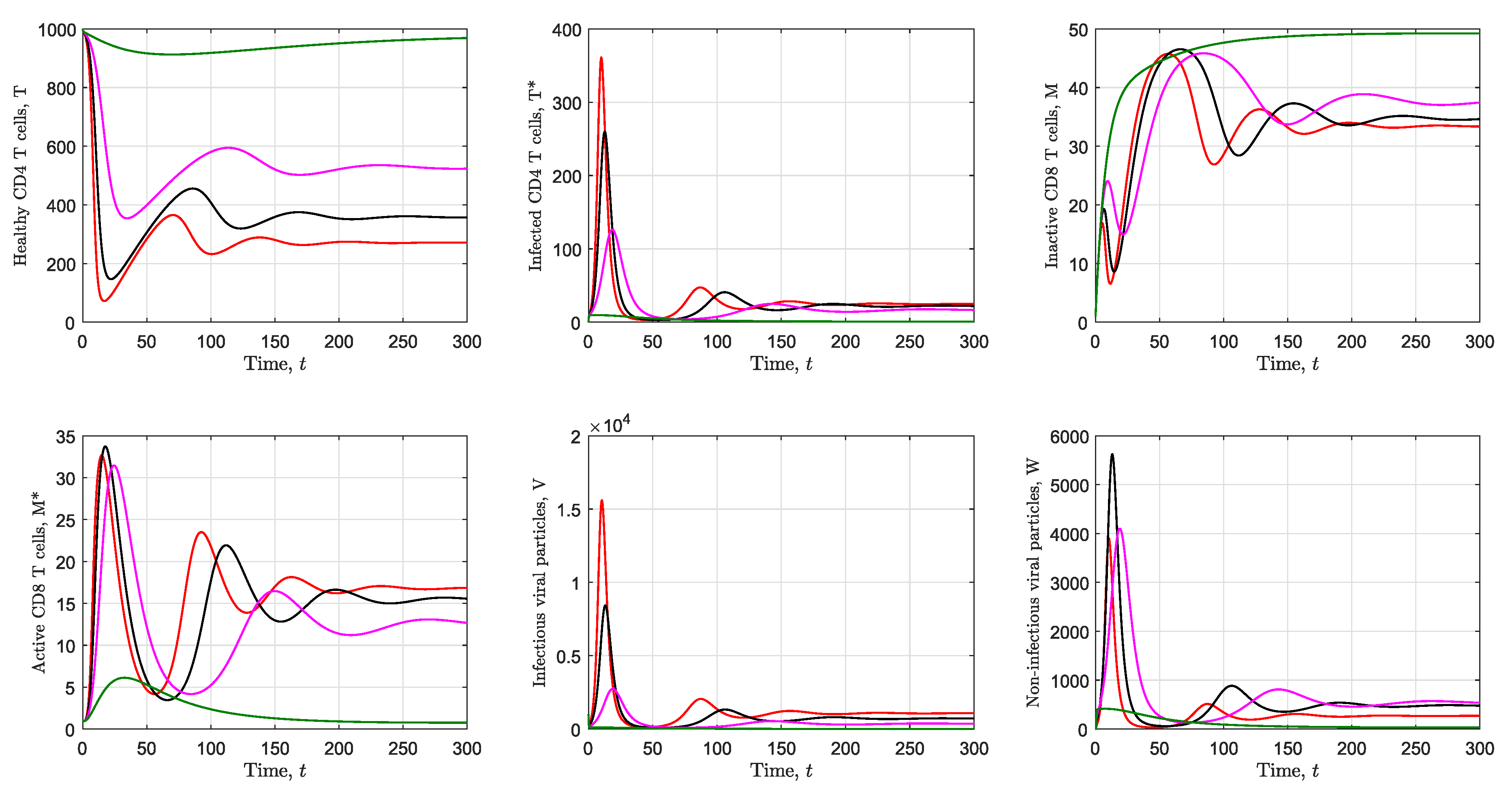
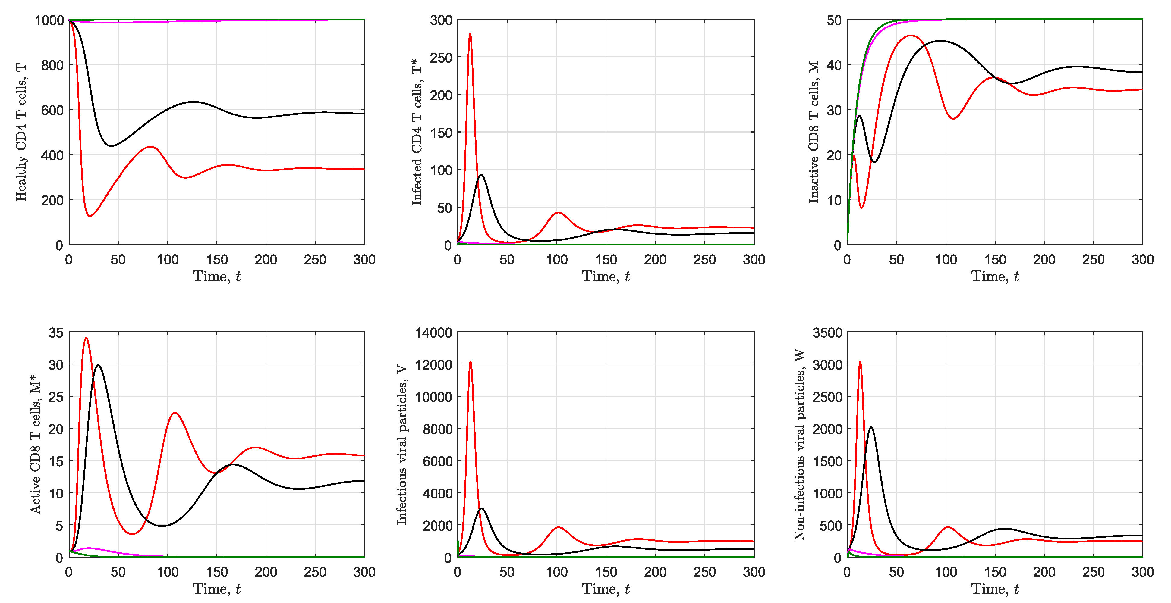
3.2. Simulation of the Immunological Model

For the purpose of studying the impact of some parameters on the system behavior, and analyzing which of them can be intervened for the infection in the immune system to be low or null, the numerical simulation of system (7) is performed by using the parameter values in Table 2 and varying the CD4 T cells infection probability β , and the probability of the active CD8 T cells eliminating the infected CD4 T cells γ (Figure 2 and Figure 3).
Figure 2 shows the variation of the CD4 T cell infection probability, β . A fixed value was used for γ = 2 × 10 3 , considering the values u 1 = 0 and u 2 = 0 that represent the effectiveness of RTI and PI, respectively, which implies no use of medications to control the infection. The red curve corresponds to β = 1.5 × 10 5 , the black curve to β = 2.5 × 10 5 , finally, the magenta and green curves represent β = 4.5 × 10 5 and β = 5.5 × 10 5 , respectively. It may be noted in the red curve (for the smaller value β = 1.5 × 10 5 ) that the number of T cells is kept at higher levels than 150 cell/mm 3 and stabilize at 358 cells. The green curve shows that for the highest value of β = 5.5 × 10 5 , the T cells remain at levels below 200 cell/mm 3 and stabilize at 100 cell/mm 3 . With respect to the number of infected cells T * , it was observed that these stabilize in the interval of ( 1 , 40 ) cell/mm 3 , for all the simulated values of β . The legend for Figure 2 shows the R 0 values obtained in each case, all greater than 1, and it was observed that the organism remains with presence of virus during the entire simulation time (active CD8 T cells M * , infected cells T * , and infectious viral particles V take values greater than zero), which illustrate the aforementioned conjecture, that is, that the equilibrium E ¯ 1 is locally asymptotically stable when R 0 > 1 . Regarding the non-infectious viral particles, it can be noted that these remain at zero during the entire simulation time because the PI are not used ( u 2 = 0 ), which leads to no production of non-infectious viral particles.
Moreover, different oscillations can be observed in each curve, in deed, when the infection begins, the body loses healthy CD4 T cells that become infected, which is why infectious viral particles also increase; then the immune system tries to recover by activating the cellular response (hence the oscillations in curves for M and M * , that are the inactive and active CD8 T cells, respectively) and increases the healthy CD4 T cell levels, decrease infected CD4 T cells and infectious viral particles. Thus, a constant battle is triggered between the immune system and the virus until, after a certain time (approximately 200 days in the simulations), the values of all cell populations and viral particles are stabilized; the same happens in the other simulations carried out in the following.
A fundamental reason for this behavior to occur is that this type of model does not describe the final phase of HIV infection, in which the diagnosis of AIDS implies that the weakened immune system allows the arrival of opportunistic diseases, which can even cause death. On the other hand, mathematically, the stability of the solutions is reached after a series of oscillations, which reflects that when analyzing the local stability of the system in a neighborhood of the equilibrium in the presence of viremia, complex eigenvalues would be obtained. This also implies that an analysis of bifurcations of the model would yield interesting results on the system’s behavior; however, such analysis is beyond the purposes of this study.
Figure 3 shows the dynamics when varying the parameter γ , which denotes the probability of active CD8 T cells M * eliminating the infected CD4 T cells T * . The simulation considers a fixed value for the infection probability β = 2.5 × 10 5 and null values for the RTI and PI effectiveness ( u i = 0 , for i = 1 , 2 ), that is, ART is not used. When taking large values of γ , i.e., γ = 9 × 10 2 (red curve) the T cells tend to stabilize at 525 cell/mm 3 approximately, infected cells T * stabilize at 15 cell/mm 3 and infectious viral particles V do so at 1000 vir/mm 3 , where they remain for most of the simulation time. On the contrary, for lower values of γ , the scenario was quite different, as expected, due to the diminished probability of the infected cells T * of being annihilated through the action of the active CD8 T cells. Thus, when simulating for γ = 2 × 10 3 (green curve) the healthy cells T tend to stabilize at 217 cell/mm 3 ; infected cells T * do so at 30 cell/mm 3 and infectious viral particles V at 3000 vir/mm 3 . It should be clarified that for every probability variation in γ , R 0 = 2.0280 was obtained, since R 0 does not depend on γ . These results also illustrate that when R 0 > 1 , there is viral presence during the entire simulation time. Note that there was no production of non-infectious viral particles, given that the PI are not used.
Observe that the variations in the infection probability of healthy cells β , and the probability of the active CD8 T cells eliminating the infected CD4 T cells γ , produce different scenarios for the infection, so that if the levels for β are high and those of γ are low, the virus will spread faster in the carrier’s organism, producing an outbreak of the infection and, vice versa, when β is low and γ is high, the virus may not establish in the body (provided R 0 < 1 ). These results basically validate the immunological model, given that they agree with known facts on the infection process and the specific cell immune response to HIV.
In Figure 4, Figure 5 and Figure 6, simulations of system (7) are conducted by varying the use of ART to control the infection, that is, the parameters that represent the effectiveness of RTI ( u 1 ) and PI ( u 2 ) are varied. Figure 4 simulates different scenarios for ART that use only the RTI, that is, varies the value of u 1 but u 2 = 0 . The values simulated for u 1 were 0.2 , 0.4 , 0.6 , and 0.8 represented by the curves in red, black, magenta, and green, respectively. Values were taken as fixed for the infection probability of the T cells ( β = 2.5 × 10 5 ), and for the probability of the active CD8 T cells eliminating infected cells T * ( γ = 2 × 10 3 ); due to the nonuse of PI, the number of non-infectious viral particles is null all the time. When simulating for high RTI effectiveness, u 1 = 0.8 (green), it is found that the infection is controlled, which is reflected by the value of R 0 = 0.7056 < 1 , and means that the immune system of the individual will be (theoretically) virus free. Additionally, the levels of infectious viral particles remained almost undetectable, that is, below 50 vir/mm 3 , the number of infected cells T * was close to zero throughout the simulation time, and the average number of active CD8 T cells was 2 cell/mm 3 . Conversely, when taking lower values for the RTI effectiveness ( u 1 = 0.2 ), the infected cells T * stabilize at 25 cell/mm 3 , the number of infectious viral particles V do so at 1500 per vir/mm 3 , the number of active CD8 T cells M * at 17 cell/mm 3 , and healthy cells T at 271 cell/mm 3 . The red curve corresponds to R 0 = 1.6224 , the black curve corresponds to R 0 = 1.3168 , and the magenta curve has R 0 = 1.0112 .
The simulation for the PI alone is shown in Figure 5 and very similar results are obtained, including the resulting value of R 0 . Fixed values were taken for the infection probability of the T cells and the probability of the active CD8 T cells eliminating infected cells T * ; thus, β = 2.5 × 10 5 and γ = 2 × 10 3 , respectively. The simulation uses u 1 = 0 and u 2 equal to 0.2, 0.4, 0.6, and 0.8 , represented by the red, black, magenta, and green curves, respectively. It may be observed that the viral particles V reach very high levels in the organism when u 2 0.6 , with these being greater than 3000 vir/mm 3 . Furthermore, the equilibrium values are in the interval of ( 500 , 2000 ) , which means an infection outbreak (in those cases R 0 was greater than 1). In spite of having varied the effectiveness of PI ( u 2 ), the results for the infected cells T * were also quite similar, almost equal to those obtained in the previous simulation (Figure 4), when using values of u 2 0.6 , T * tends to stabilize in the interval ( 5 , 30 ) cell/mm 3 , and the active CD8 T cells stabilize in the interval ( 13 , 17 ) . The most notable difference between both simulations performed for the RTI and PI effectiveness is that for the first (Figure 4), the levels of non-infectious viral particles is zero for the entire time, as expected. Indeed, defective viral particles are not produced, which does occur when PI are used (Figure 5). Moreover, it is observed, with the assumptions considered here, that when reaching PI effectiveness in the interval ( 0.8 , 1 ) the viral load becomes undetectable and very high values of healthy cells T are reached.
Figure 6 shows the simulation to control the virus by using RTI ( u 1 ) and PI ( u 2 ), simultaneously, under the assumption that u 1 = u 2 for convenience and simplicity. The values used were 0.2, 0.4, 0.6, and 0.8 represented by red, black, magenta and green curves, respectively. In addition, fixed values are taken for the infection probability of the T cells and the probability of active CD8 T cells eliminating infected cells T * , being β = 2.5 × 10 5 and γ = 2 × 10 3 , respectively. The panorama of the infection in this simulation is totally different from that shown in Figure 4 and Figure 5, given that in this case, HIV does not spread in the same magnitude; indeed, for values of RTI and PI effectiveness above 0.6 (magenta and green curves), the viral load is not detectable for both infectious and non-infectious viral particles, the infected cells T * are in values practically null and the number of active CD8 T cells per mm 3 remains for most of the simulation time very close to zero, which is why the green and magenta curves are over the horizontal axis. Note also that healthy cells T remain close to 1000 cell/mm 3 when effectiveness in using RTI and PI are 0.6 . Additionally, when said effectiveness takes on values 0.4 (red and black curves), the infected cells T * stabilize at interval ( 1 , 50 ) cell/mm 3 , the infectious viral particles stabilize at interval ( 100 , 1500 ) vir/mm 3 , and the non-infectious viral particles stabilize at interval ( 100 , 500 ) vir/mm 3 ; lastly, it is worth highlighting that the values obtained of R 0 in those cases are less than 1, as reported in the figure legend, which illustrates the result of the Proposition 2.
With the foregoing, it can be stated that when using different types of inhibitors to combat HIV, the results are much more encouraging when seeking to suppress viral load and diminish the rate at which the virus spreads within the organism of each carrier. With the parameters considered here, when the effectiveness of RTI and PI take on high values (> 0.6 ), small values for R 0 are achieved and, therefore, low levels of infected CD4 T cells, active CD8 T cells, and viral particles are achieved. Once again, these results permit validating the model, evidencing that using different inhibitors in combination is more convenient than using them in an isolated manner.

3.3. Coupling Algorithm of the Immunological and Population Scales

For the purpose of coupling the model in the immunological scale (system of differential equations) with the model for the propagation in the population scale (complex network), an algorithm was designed that permits manipulating the complex network, so that events in the population scale, that is, the way the virus will spread in the population, are influenced by the immune status of each individual.
1.
The network was constructed by beginning with the random values [38,39,40] shown in the following, which seeks for each individual i, for i = 1 , , N T , from the network to have a different immune system. Additionally, for the values of the other parameters used in the system of differential equations that describe the immunological scale, those described in Table 2 were used.
(a)
Initial number of healthy CD4 T cells in the i-th person per mm 3 : T i ( 0 ) [ 200 , 1000 ] .
(b)
Initial number of inactive CD8 T cells in the i-th person per mm 3 : M i ( 0 ) [ 70 , 980 ] .
(c)
Values of infected CD4 T cells, active CD8 T cells, infectious and non-infectious viral particles will be null, given that it is considered that the i th person is still not infected by the virus, that is, T i * ( 0 ) = M i * ( 0 ) = V i ( 0 ) = W i ( 0 ) = 0 .
(d)
Production rate of healthy cells of the i-th person: σ i [ 5 , 20 ] .
(e)
Infection probability of the healthy cells of the i-th person: β i [ 0 , 2.5 × 10 5 ] .
(f)
Production rate of viral particles of the i-th person: N i [ 100 , 1500 ] .
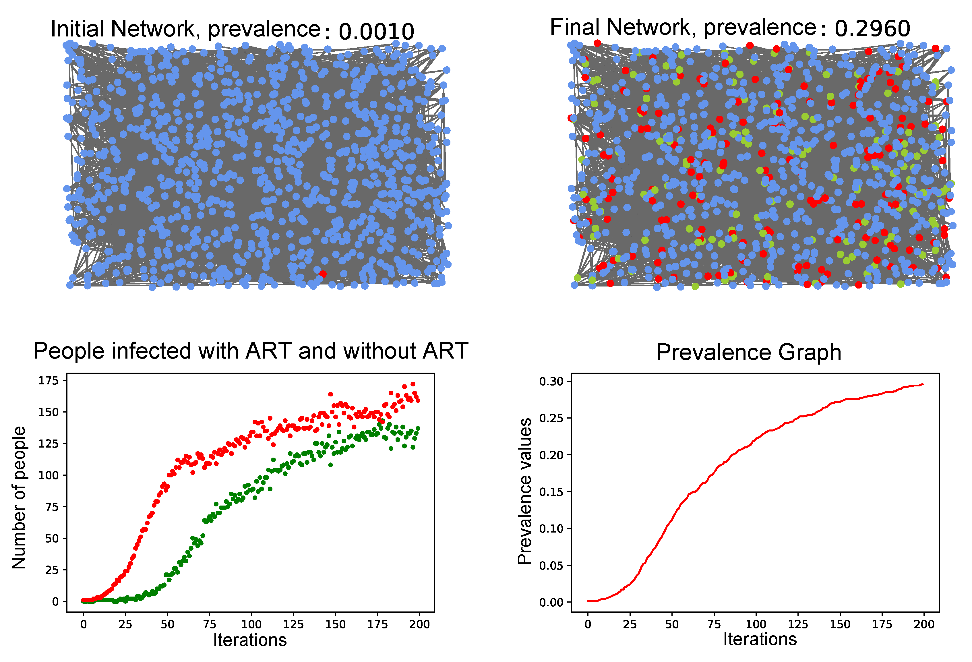
Then, a vertex from the network is chosen randomly as the first infected and is assigned a random viral load between 1 and 1000 vir/mm 3 [41]. With the aforementioned, the network is created, obtaining the initial state at τ = 0 .
2.
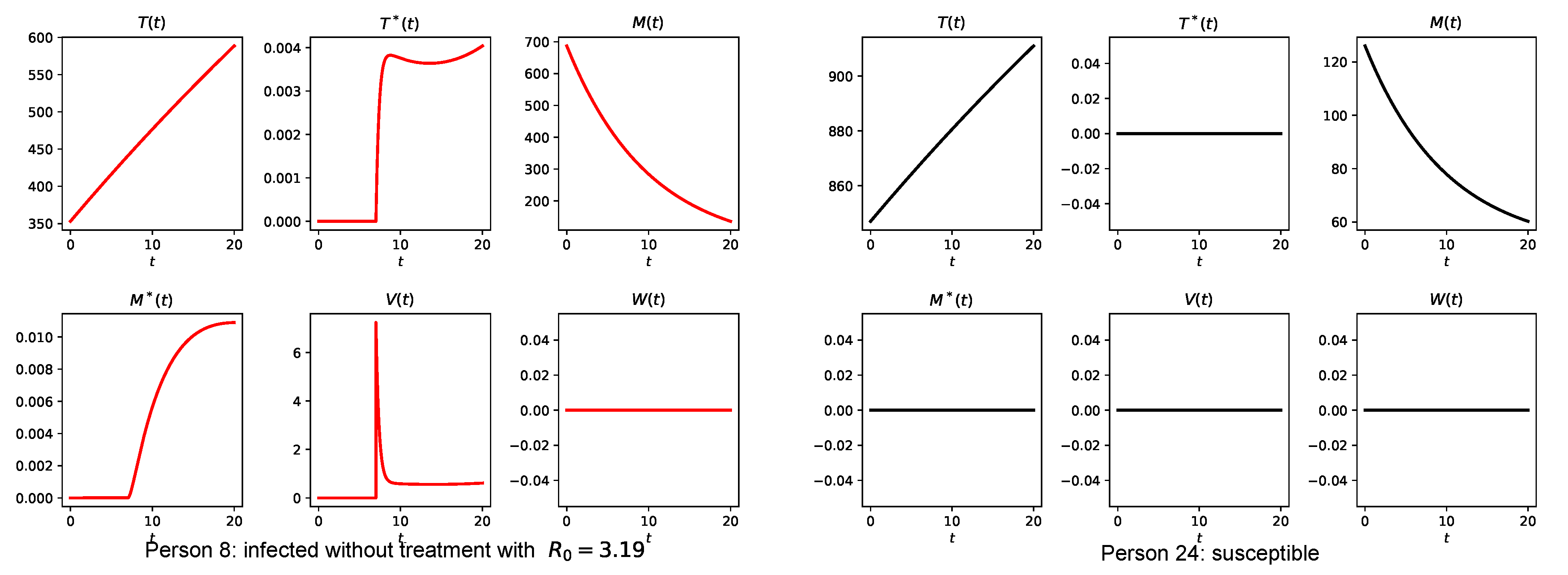
From the corresponding initial condition, we solve the system of differential equations of the immunological system (7) for each vertex i during one unit of time, saving the numerical solutions T i ( t ) , T i * ( t ) , M i ( t ) , M i * ( t ) , V i ( t ) and W i ( t ) ; therefore, we have the immunological status of each individual in the population during that unit of time. Additionally, the final value of each of the numerical solutions will be used as the initial condition in the following iteration. Furthermore, we saved the number of susceptible subjects, carriers with ART and carriers without ART at the end of the iteration.
3.
Based on the numerical solutions, the following decisions were made:
(a)
If the i-th person is an HIV carrier and presents a number of healthy CD4 T cells T i below 350 cell/mm 3 , a random probability of accessing to ART is assigned, if it is > 0.6 , it is established to use ART, so that a random value is assigned for u 1 and u 2 between ( 0 , 1 ) .
(b)
If the i-th person is an HIV carrier already using ART, a random probability of therapy abandonment is assigned, if it is < 0.2 , it is established that the individual leaves ART, that is u 1 = u 2 = 0 .
This is why in the simulations that will be presented ahead in different iterations, the state of the vertices will vary from carriers with therapy to carriers without therapy, and vice versa.
4.
The transmission process considers different factors. If the i-th person is an HIV carrier, the decision is made randomly whether to have a sexual encounter with only one of their susceptible “neighbors” (another susceptible vertex sharing an edge). If the random decision was affirmative, the infected person is partnered with one of their susceptible sex partners, then, the probability of transmitting the infection from the infected person i to the susceptible person j is given by λ i j = i j λ i k (taken from [16]), where k represents the average degree (associated with the potential number of sex partners) and λ i is the infection probability through sexual contact; the probability λ i is taken from [40] and is shown in Table 3 according to the values of vir/mm 3 .
Finally, if person j becomes infected, an initial viral load is assigned with 10% of the load owned by the person i who caused the infection.
5.
At the end of each iteration, the prevalence was calculated, as the rate between the number of HIV carriers with or without therapy and the total number of people from the network, that is,
P f = y i + z i x i + y i + z i .
The algorithm described is conducted until τ = τ f , the total number of iterations.

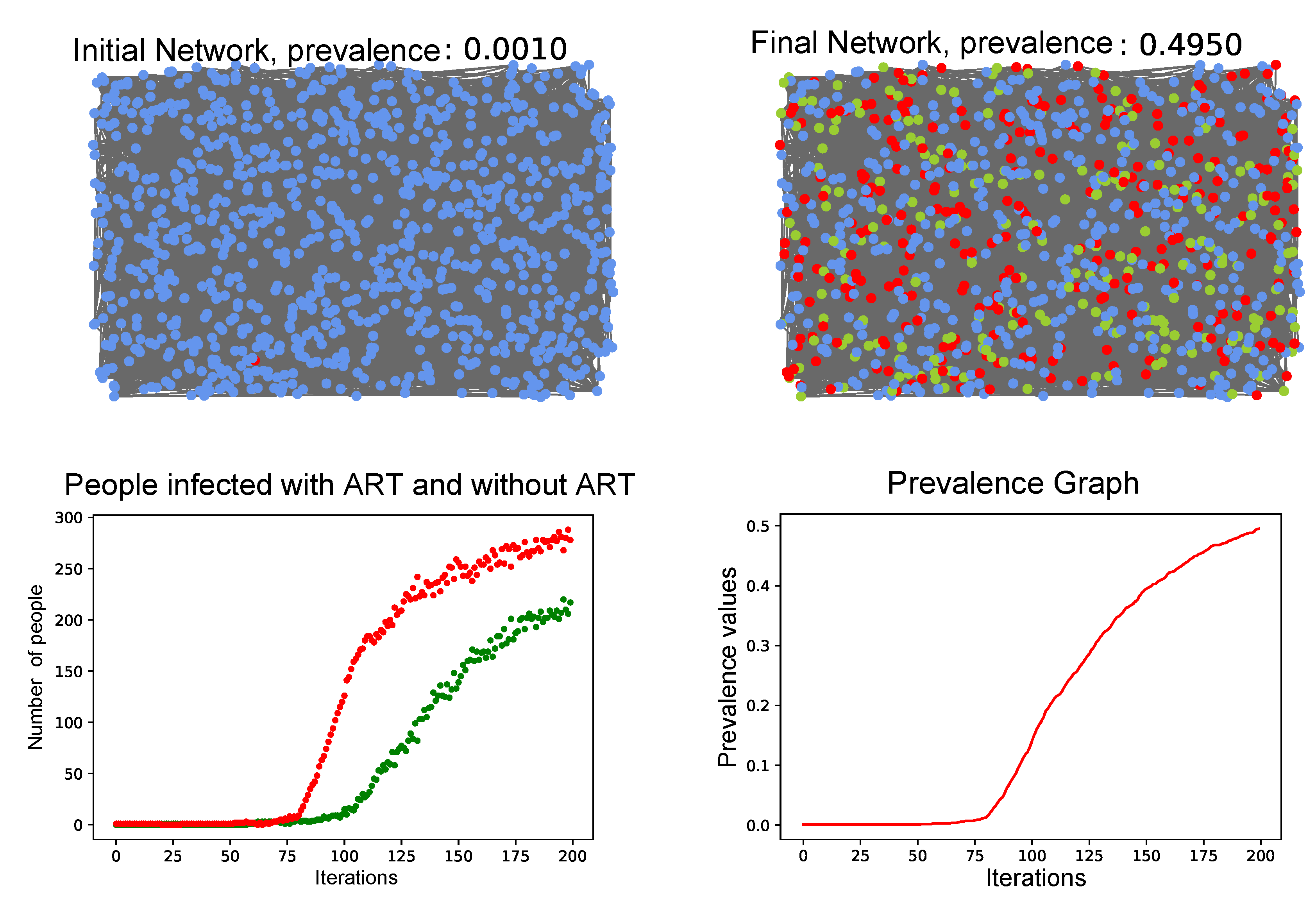
3.4. Simulation of the Coupled Model

To illustrate the coupled model, a simulation shown in Figure 7 was performed for N T = 25 people, k = 2 , and τ f = 20 iterations, and the corresponding immune status of selected nodes is presented in Figure 8; additionally, two more simulations are shown for N T = 1000 , τ f = 200 , k = 4 (Figure 9), and k = 10 (Figure 10). Those simulations illustrate the implementation of the model and do not intend to reflect real scenarios. In each case, the blue vertices represent people susceptible of acquiring HIV x i , those in red represent HIV carriers without therapy y i , and those in green represent HIV carriers taking ART z i .
Figure 7 shows the initial network, iterations 2, 6, 10, 11, 12, 13, 14, 17, and the final network; hence, it shows the infection’s spread over time, obtaining a final prevalence P f = 0.68 (again, this simulations are for illustration purposes only). The first vertex infected is 19; at iteration 6, it manages to infect vertex 8. Then, at iteration 10 the number of HIV carriers has increased because vertices 2 and 5 are the new ones infected. Later, at iteration 14, the number of HIV carriers is seven (vertices 1, 2, 5, 8, 9, 19, and 21). Lastly, the network ends with 17 people infected, from which two are taking ART (vertices 5 and 19 in green). Note that during the simulation time, vertex 19 accessed therapy and abandoned it on several occasions (in iterations 2, 10, 12, and 14, vertex 19 accessed ART, and abandoned it in iterations 6, 11, and 13). Vertex 5 was without therapy and accessed it in iteration 17. As mentioned, the numerical solutions of each person’s immune system were saved for each iteration of the network; hence, Figure 8 shows the cell populations T, T * , M, M * and viral loads V and W of individuals 1, 8, 19, and 24 of the network simulated in Figure 7, as an example. Black curves mean the person remained susceptible during the entire simulation time; red represents a person who is an HIV carrier and who in the final time τ f did not take ART; lastly, green represents a person who is an HIV carrier and who in the final time τ f uses ART. Note that each person began with a different number of T and M cells, which guarantees that a different immune system is considered for each one (numeral 1 of the previous subsection).
The simulation presented in Figure 8 shows the immune system of person 19, who was the first infected, upon ending the simulation time this person took ART (green). In the curves of viral particles V and W it may be estimated that ART had begun since iteration 2, but it is seen that therapy is alternatively taken and interrupted from iteration 10, which is revealed by the abrupt oscillations shown. As expected, when abandoning ART, HIV manages to replicate and high levels of viremia are reached. Furthermore, it is observed that person 19, during most of the simulation time, maintained low levels of healthy cells T, below 360 cell/mm 3 . Person 8 acquired the virus during an early stage of the simulation (iteration 6); this is why for τ = 7 its T * and M * cells and viral particles V began to reach high levels, also notice that this person started using RTI at iteration 9, but never used the PI during the simulation time, which is why the W values remain at zero. Upon ending the simulation time, this person did not take ART. It is also observed that, although person 8 is infected, the number of healthy cells T did not diminish at any moment during the simulation period, a situation that possibly would change if we increase the number of iterations. Person 1 did not use the PI at any moment of the simulation, which is why the number of non-infectious viral particles W remained at zero; furthermore, it is noted that this person acquired the infection almost at the end of the simulation (iteration 14), but in spite of that achieved an R 0 = 12.15 ; it could be inferred that, upon increasing the number of iterations, and if this person remains without taking ART, the viral spread will be accelerated, generating an infection outbreak and which would cause a much greater probability of infecting their susceptible sex partners and of the virus spreading faster in the population. In fact, although person 1 was infected in the almost final stage, its infectious viral particles V reached high values (note the high value of R 0 ). Finally, Person 24 is susceptible, hence, during the simulation time was never infected with HIV and this is the cause for only T and M cell populations having values different from zero.
Figure 9 shows the simulation for a bigger population with N T = 1000 , a higher number of iterations τ f = 200 , and takes γ = 3.4 from the literature [17,27]. This simulation refers to a slightly conservative population, given that it has been assigned a maximum number of sex partners of k = 4 . Figure 9 shows the initial network with the first vertex infected (red upper-left panel), the final network (upper-right panel), the plot showing the population of HIV carriers taking ART (green dots) and those not taking it (red dots) located on the lower left panel and, finally, the prevalence (lower-right panel). The plot for both HIV carrier populations with and without therapy is constructed by accounting for the number of people in the different states (susceptible, infected with ART, and infected without ART) in each iteration; we obtained, as a result, sequences of points that tended to stabilize over time, with the red curve being greater or equal to the one in green most of the time, which means that y i < z i . It may be inferred from the plot that both populations tend to stabilize at an equilibrium value: for the first, that equilibrium value is around 160 people, that is, 16 % of the HIV carriers take ART at the end of simulation, while for the population of HIV carriers without ART, the equilibrium point is around 135 people, that is, 13.5 % of the HIV carrier population does not take ART at the end of the simulation. This situation is repeated in all the simulations we performed, although, here, we are assuming the probability of accessing ART as 0.6 and the probability of abandoning ART as 0.2. This is an interesting result indicating that the number of people who do not access ART being higher than those who access ART is an interesting source of information that should be studied in more detail. The prevalence plot (lower-right panel) provides an approximate idea of when the virus spread may have started. In this case, it is observed that it was close to iteration 5. The prevalence values are found through Equation (10) computed at each iteration. It is necessary to highlight that the prevalence plot grows in its entire domain and this is due to HIV not having a cure; hence, a virus carrier, with or without therapy, cannot go on to become a susceptible person; in the simulation, the final prevalence value was 0.2960 .
Figure 10 shows the simulation of a more liberal population, where the average number of sex partners is k = 10 , taking the same amount of people for the population and the same number of iterations, that is, N T = 1000 and τ f = 200 , respectively, and γ = 3.4 was again taken from the literature [17,27]. Figure 10 also shows the initial network with its first infected (upper left panel), the final network (upper right panel), the graphic showing the relation between people infected with and without ART (lower-left panel), and the prevalence plot (lower-right panel). In the final network, a prevalence of 0.4950 is achieved, which is quite high and means that 49 % of the population are HIV carriers. This simulation shows a scenario where people have a large number of sex partners and use no protection. It is noteworthy that it was used k = 10 , because a population of 1000 young people between 15 and 24 years of age is considered, in a simulation time of 200 weeks (approximately 4 years), so it is not unreasonable to think that a person from a slightly more liberal population could have an average of 10 sexual partners in a 4-year period. In comparison, with the simulation shown in Figure 9, it is evidenced that values of k may cause the network to become susceptible to changes in the rate at which the virus spreads. Due to the aforementioned, the infection prevalence in the slightly conservative population with k = 4 was lower than that obtained in the more liberal population with k = 10 . Analogous to the previous simulation, for the graphic showing the relation between the population of carriers not taking ART and those taking it (lower-left panel), the population not taking ART continues being more numerous during the entire simulation time; additionally, this population tends to stabilize over time at values close to 270 people, approximately, this is 27 % of the total population, unlike the population of people infected who take ART, in which the equilibrium value is reached around 210 people, that is, 21 % of the 1000 people; again, this proves a higher number of people who do not have access to ART. The prevalence plot (lower-right panel) shows that close to iteration 50, virus spread begins to accelerate, the curve growth is more pronounced (greater slope) and, finally, the curve starts reducing (the slope diminishes) towards the end, indicating fast virus spread followed by slow propagation. It is also noted that this plot presents an equilibrium point, which coincides with the prevalence value in the final time τ f . Although in the simulation for a conservative population, the infection outbreak occurred in time τ = 5 , the prevalence was lower than the simulation made for a more liberal population, where the infection outbreak took place over later time, for τ = 50 .

4. Conclusions

This paper studies a multi-scale model for HIV propagation in a group of people between 15 and 24 years of age, through a cluster-type scale-free complex network, which follows a power law. The model relates the immunological scale with the population scale so that the information obtained from the immunological scale helped to model decision making on how the infection would spread in the population.
At an immunological level, the infection is controlled when reducing the probability of healthy CD4 T cells becoming infected. Thereby, when small values are achieved in said probability, the infection remains in low levels. It was also evidenced that when the cellular immune response has a high probability of eliminating infected cells, the infection can be controlled; essentially, these results validate the model, because they correspond with known facts about the infection process and the specific cell immune response to HIV. The model analysis reflects how the use of reverse transcriptase inhibitors (RTI) and protease inhibitors (PI) helps to control infection in the immune system of each HIV carrier, as well as in the spread of the infection within the population. Therapies help to reduce viral outbreaks, and evidence that when using different types of ART, at the same time, better results are achieved than using them in isolated manner, which again validates the model for the immunological scale studied here. Lastly, with the assumptions of the immunological model, and the values of the parameters used in the simulations, it was observed that when reaching combined ART effectiveness in the interval ( 0.6 , 1 ) , the viral load becomes undetectable and large values are reached for the healthy CD4 T cells.
Different scenarios were found in the immune system’s simulations for the population scale. The first deals with people uninfected during the entire simulation period, which is why there are only values in the number of healthy cells T and inactive cells of the cellular response M, while cellular and viral values remain null. Another scenario is that shown by people who take ART, but only use the RTI, which is why the non-infectious viral particles W are shown in zero. A very characteristic scenario was found, that of HIV carriers who take and abandon therapy on alternate occasions during the simulation period, which is why we get graphics with maximums and minimums in form of abrupt peaks. Finally, another scenario related with R 0 , is that showing that when large values are obtained (>1), the infection spreads faster in the organism of each carrier, unlike a low R 0 , which keep the HIV from propagating quickly, or that (theoretically) the person is not infected when R 0 < 1 , scenarios that can be associated with undetectable viral loads.
Moreover, it is observed from simulations that a higher number of sex partners a person has within a specific population, means a higher prevalence of the virus within said population, and that the infection will spread at higher rates, as long as the sexual encounters are unprotected. Additionally, in simulations that relate the number of HIV carriers with and without ART, we obtained sequences of points that tended to stabilize over time and, in all the cases simulated, the population of HIV carriers without ART was greater or equal to those with ART. This reflects an interesting relation between access and abandonment of ART, which is something we cannot explain as a consequence of the parameters considered here, indeed, the simulations consider the probability of ART access as 0.6 , and the probability of ART abandonment as 0.2 . Further studies should be performed in this regard. Nevertheless, our coupling algorithm of the immunological scale with the population scale takes random probabilities for access and abandonment of ART for each HIV carrier at each iteration; thus, we consider that for future research the most adequate would be to assign these values in non-random manner, using the viral load and the CD4 T cell count.
Regarding the prevalence, to obtain large values it is not necessary to start viral propagation during early stages of the simulation. This is due to many factors that influence decision making on the mode of virus spread in the model (it may occur that, although the first person is infected over early time of simulation, small prevalence values may be obtained); thus, it may be inferred that much uncertainty exists when not knowing clearly how the virus will spread and which variables to take into account in such modeling decisions. In addition, although equal values are used for the parameters, each simulation will lead to different prevalence results and a different virus propagation behavior, however, in a constant population, prevalence will tend to an equilibrium point (approximately the final value in simulations), this suggest that future works should conduct multiple simulations, with the same parameter values, to statistically infer the prevalence expected value for that parameter configuration.
Finally, it is believed that the formulation of this mathematical model is adequate, given that the assumptions made when modeling the spread of HIV, are improved by taking into account the two scales (immunological and population). Indeed, the multi-scale model studied here adds to the available literature an overview of what the dynamics of infection in a population would be like if the immune status of people within said population were considered, and serves as the basis for future research that seeks to consider more variables to achieve a model closer to reality. It is necessary to clarify that the parameter values used in the simulations (mainly from secondary sources) and the resulting data do not seek to show a real picture of HIV propagation in any specific population, because the main objective was the model’s description and its relevance. Only by comparing the real data worldwide, there are around 7.9-billion people [42] in the world, if the number of HIV carriers is considered as reported by [3], the prevalence as calculated here will result in approximately 0.005; however, models of this nature would allow us to explore the HIV propagation in population groups with specific risks in greater detail.

Author Contributions

Conceptualization, H.D.T.-Z. and S.d.A.V.-Q.; methodology, H.D.T.-Z.; software, H.D.T.-Z. and S.d.A.V.-Q.; validation, H.D.T.-Z., S.d.A.V.-Q. and D.A.P.-M.; writing: original draft, S.d.A.V.-Q.; writing: revision and editing, H.D.T.-Z., S.d.A.V.-Q. and D.A.P.-M.; supervision, H.D.T.-Z. All authors have read and agreed to the published version of the manuscript.

Funding

This research was funded by Universidad del Quindío through research project 922.

Acknowledgments

H. D. Toro-Zapata and S. A.Vásquez-Quintero were supported by Universidad del Quindío through research project 922.

Conflicts of Interest

The authors declare having no conflict of interest.

Abbreviations

The following abbreviations are used in this manuscript:
HIVHuman Immunodeficiency Virus
AIDSAcquired immune deficiency syndrome
ARTAntiretroviral therapy
RTIReverse transcriptase inhibitors
PIProtease Inhibitors
LAElocally asymptotically stable
SymSymbol

Appendix A. Demonstration of Propositions and Basic Reproduction Number

Proof of Proposition 1.
Starts by demonstrating that for each coordinated hyperplane of R 6 (if the initial conditions are non-negative and considering that 0 u i 1 by definition, with i = 1 , 2 ) the solutions are found in the non-negative octant of R 6 , in deed:
T ˙ T = 0 = σ β ( 1 u 1 ) ( 0 ) V μ ( 0 ) = σ > 0 T * ˙ T * = 0 = β ( 1 u 1 ) T V γ ( 0 ) M * δ ( 0 ) = β ( 1 u 1 ) T V 0 M ˙ M = 0 = λ ψ T * ( 0 ) ρ ( 0 ) = λ > 0 M * ˙ M * = α T * ( 0 ) ρ ( 0 ) + ψ T * M = ψ T * M 0 V ˙ V = 0 = N δ ( 1 u 2 ) T * c ( 0 ) = N δ ( 1 u 2 ) T * 0 W ˙ W = 0 = N δ u 2 T * c ( 0 ) = N δ u 2 T * 0 .
Now, it is guaranteed that the solutions are bound above. For V = 0 in (1) we obtain:
T ˙ σ μ T T ˙ + μ T σ .
Then, T ( t ) σ μ + k e μ t , hence lim t T ( t ) lim t σ μ + k e μ t = σ μ . Thus, T σ μ . Furthermore, if G = T + T * + M + M * , then:
G ˙ = σ β ( 1 u 1 ) T V μ T + β ( 1 u 1 ) T V γ T * M * δ T * + λ ψ T * M ρ M + α T * M * + ψ T * M ρ M * = σ μ T γ T * M * δ T * + λ ρ M + α T * M * ρ M * = σ + λ + α T * M * γ T * M * ( μ T + δ T * + ρ M + ρ M * ) σ + λ + ( α γ ) T * M * ε ( T + T * + M + M * ) ; with ε = max { μ , δ , ρ } σ + λ ε G + ( α γ ) T * M * , supposing γ α σ + λ ε G ( γ α ) T * M * σ + λ ε G .
Through an analogous process as the used to bound the T variable, we obtain that G ( t ) σ + λ ε , hence, particularly T * ( t ) σ + λ ε .
Finally, if D = V + W , then:
D ˙ = N δ ( 1 u 2 ) T * c V + N δ u 2 T * c W = N δ T * ( 1 u 2 + u 2 ) c ( V + W ) = N δ T * c D N δ σ + λ ε c D N δ ( σ + λ ) ε c .
It is then obtained that D ( t ) N δ ( σ + λ ) ε c , this completes the proof. □
Deduction of the basic reproduction number. To find the R 0 of model (7), we define vectors h and g, corresponding to the equations of the populations responsible for the infection:
h = β ( 1 u 1 ) T V γ T * M * 0 ,   g =   δ T * N δ ( 1 u 2 ) T * c V .
The next-generation matrix is defined as M ˜ = H G , where H = D h and G = ( D g ) 1 . For D h and D g , the respective Jacobian matrices of h and g with respect to T * and V. In this case,
H = h T * h V 0 0 = γ M * β ( 1 u 1 ) T 0 0 ,
and,
G = g T * g V g T * g V 1 = 1 δ 0 N δ ( 1 u 2 ) δ c 1 c .
Therefore, M ˜ , the next-generation matrix, remains,
M ˜ = H G = γ M * δ + β N δ ( 1 u 1 ) ( 1 u 2 ) T δ c β ( 1 u 1 ) T c 0 0 .
Then, M ˜ evaluated in the virus-free equilibrium E 0 ¯ σ μ , 0 , λ ρ , 0 , 0 , 0 yields as result:
M ˜ = σ β N ( 1 u 1 ) ( 1 u 2 ) μ c σ β ( 1 u 1 ) μ c 0 0 .
Finally, the eigenvalues of this matrix are z 1 = 0 and z 2 = σ β N ( 1 u 1 ) ( 1 u 2 ) μ c , hence, the spectral radius is given by:
R 0 = p ( M ˜ ) : = max 0 , σ β N ( 1 u 1 ) ( 1 u 2 ) μ c = σ β N ( 1 u 1 ) ( 1 u 2 ) μ c ,
which corresponds to the basic reproduction number.
Proof of Proposition 2.
To study the local stability, linearization of the system is performed around the equilibrium point E 0 ¯ and E 1 ¯ . First, the Jacobian matrix is evaluated in the virus-free equilibrium E 0 ¯ = σ μ , 0 , λ ρ , 0 , 0 , 0 , whose characteristic polynomial is given by:
p ( z ) = ( μ z ) ( c z ) ( ρ + z ) Q ( z ) ,
where,
Q ( z ) = z 3 + ( ρ + δ + c ) z 2 + δ ρ + c ρ + δ c σ μ F z + δ c ρ σ μ ρ F .
By solving p ( z ) = 0 we obtain three negative eigenvalues, z = μ ; z = c ; z = ρ and a cubic equation
Q ( z ) = 1 δ c z 3 + ρ + δ + c δ c z 2 + ρ c + ρ δ + 1 R 0 z + ρ ( 1 R 0 ) = 0 .
If R 0 < 1 , then (A1) does not have any sign changes in its coefficients, then, by Descartes’ rule [43], the roots of the cubic equation are all negative and E ¯ 0 is locally asymptotically stable (LAE). If R 0 > 1 , the coefficient ρ ( 1 R 0 ) < 0 and the coefficient ρ c + ρ δ + 1 R 0 could be positive or negative, in any case, the equation will only have a change of sign and there will be a positive root, hence, the virus-free equilibrium E 0 ¯ is unstable.
Now, upon evaluating the Jacobian matrix on the equilibrium E 1 ¯ = T ¯ , T * ¯ , M ¯ , M * ¯ , V ¯ , W ¯ , it is found that the characteristic polynomial has the form:
p ( z ) = A 0 z 6 + A 1 z 5 + A 2 z 4 + A 3 z 3 + A 4 z 2 + A 5 z + A 6
Given that algebraic difficulties arise when trying to find the eigenvalues, it is established as a conjecture that E 1 ¯ is LAE when R 0 > 1 , which will be illustrated numerically. □
Proof of Proposition 3.
To study the number of positive roots of Equation (9), we keep in mind Descartes’ Rule again; hence, there would be no positive roots if B and C are at the same time positive. Thus, it will be proven that B C < 0 as long as R 0 > 1 and α < ψ , in deed, it is obtained that R 0 > 1 c μ δ < σ F
B = γ λ ψ F + δ F ρ ( α ψ ) α ψ σ F + α ψ μ δ c γ λ ψ F + δ F ρ ( α ψ ) α ψ σ F + α ψ σ F < 0
For the case α > ψ and R 0 > 1 , we obtain C < 0 ,
C = δ ρ 2 F c μ γ λ ψ + c μ δ ρ ( α ψ ) σ F ρ ( α ψ ) < δ ρ 2 F c μ γ λ ψ + c μ δ ρ ( α ψ ) c μ δ ρ ( α ψ ) , because R 0 > 1 c μ δ < σ F = δ ρ 2 F c μ γ λ ψ < 0
This prove that if R 0 > 1 , B and then C have contrary signs, that is, B C < 0 . Given that B < 0 or C < 0 , there are two sign changes in Equation (9), according to Descartes’ Rule there will be a maximum of two positive roots. If there are two positive solutions, these are assumed as T ¯ 1 * and T ¯ 2 * , where T ¯ 1 * < T ¯ 2 * . We then have:
1.
There are two positive solutions, that is, two endemic equilibriums if T ¯ 1 * and T ¯ 2 * satisfy the conditions to obtain M ¯ * > 0 (see (8)); that is:
0 < T 1 * ¯ < T 2 * ¯ < ρ α .
2.
There are no positive solutions, that is, there is no endemic equilibrium if T 1 * ¯ and T 2 * ¯ fulfill:
ρ α < T 1 * ¯ < T 2 * ¯ .
3.
There is a single endemic equilibrium point if T 1 * ¯ and T 2 * ¯ fulfill:
0 < T 1 * ¯ < ρ α < T 2 * ¯ .
To satisfy Equations (A1) and (A2), it must be fulfilled that when evaluating in the cubic Equation (9) the value of ρ α is > 0; however, by evaluating ρ α in Equation (9) it remains:
A ρ α 3 + B ρ α 2 + C ρ α + D = 0 δ ψ F ρ 3 α 2 + δ F ( α ψ ) ρ 3 α 2 γ λ ψ F ρ 2 α 2 + ψ ( δ c μ σ F ) ρ 2 α δ F ρ 3 α = 0 c μ γ λ ψ ρ α + δ c μ ( α ψ ) ρ 2 α + F σ ( ψ α ) ρ 2 α + σ F ρ 2 δ c μ ρ 2 = 0 γ λ ψ F ρ 2 α 2 c μ γ λ ψ ρ α < 0 .
Hence, the equation is fulfilled (A4) and it is concluded that if R 0 > 1 , a single point of equilibrium exists in presence of virus in the system, which is E 1 ¯ = T ¯ , T ¯ * , M ¯ , M ¯ * , V ¯ , W ¯ given by (8).   □

References

  1. AIDS InfoNet. Available online: http://www.aidsinfonet.org/uploaded/factsheets/204_spa_485.pdf (accessed on 22 May 2018).
  2. Organización Mundial de la Salud. Available online: https://www.who.int/features/factfiles/hiv/es/ (accessed on 14 February 2019).
  3. UNAIDS. Available online: https://www.unaids.org/es/resources/documents/2021/UNAIDS_FactSheet (accessed on 23 August 2021).
  4. InfoSIDA. Available online: https://www.infosida.es//que-es-el-vih (accessed on 26 March 2018).
  5. Planas, G. La infección por el virus de la inmunodeficiencia humana. In Farmacia Hospitalaria Tomo II, 3rd ed.; Fundación Española de Farmacia Hospitalaria: Madrid, Spain, 2002; pp. 1493–1516. [Google Scholar]
  6. Dirección general de comunicación por los derechos humanos de la CDHDF. VIH un llamado a la acción positiva. Dfensor 2014, 2, 5–19. [Google Scholar]
  7. Velasquez, S.; Bedoya, B. Los jóvenes: Población vulnerable del VIH/SIDA. Med. UPB 2010, 29, 144–154. [Google Scholar]
  8. UNAIDS. Available online: http://data.unaids.org/topics/young-people/youngpeoplehivaids_es.pdf (accessed on 25 May 2018).
  9. Comisión Nacional de los Derechos Humanos México. Available online: https://www.cndh.org.mx/sites/default/files/doc/Programas/VIH/Divulgacion/cartillas/Cartilla-DH-Jovenes-VIH-Sida.pdf (accessed on 14 April 2018).
  10. Instituto Nacional de Salud. Boletín Epidemilógico Semanal, Semana epidemiológica 47, 17 al 23 de Noviembre de 2019. Available online: https://www.ins.gov.co/buscador-eventos/BoletinEpidemiologico/2019_Boletin_epidemiologico_semana_47.pdf (accessed on 29 September 2020).
  11. CATIE. Available online: https://www.catie.ca/en/fact-sheets/transmission/hiv-viral-load-hiv-treatment-and-sexual-hiv-transmission (accessed on 23 August 2021).
  12. UNAIDS. Available online: https://www.unaids.org/sites/default/files/media_asset/JC2484_therapy-2015_es_1.pdf (accessed on 7 January 2018).
  13. Toro-Zapata, H.D.; Vasquez-Roa, E.M.; Mesa-Mazo, M.J. Modelo estocástico para la infección con VIH de las células CD4 T+ del sistema inmune. Rev. Mat. Teor. Apl. 2017, 24, 287–313. [Google Scholar] [CrossRef] [Green Version]
  14. Toro-Zapata, H.D.; Rodríguez-Osorio, A.J.; Medellín-Prieto, D.A. Modelo para el acceso efectivo al tratamiento antirretroviral en relación con el fracaso terapéutico de la infección por VIH. Rev. EIA 2019, 16, 115–130. [Google Scholar] [CrossRef] [Green Version]
  15. Barabási, A.L.; Albert, R. Emergence of scaling in random networks. Science 1999, 286, 509–512. [Google Scholar] [CrossRef] [Green Version]
  16. May, R.M.; Lloyd, A.L. Infection dynamics on scale-free networks. Phys. Rev. E 2001, 64, 066112. [Google Scholar] [CrossRef] [PubMed] [Green Version]
  17. Newman, M.E.; Barabási, A.L.E.; Watts, D.J. The Structure and Dynamics of Networks; Princeton University Press: Princeton, NJ, USA, 2006; pp. 1–8. [Google Scholar]
  18. Sloot, P.M.; Ivanov, S.V.; Boukhanovsky, A.V.; van de Vijver, D.A.; Boucher, C.A. Stochastic simulation of HIV population dynamics through complex network modelling. Int. J. Comput. Math. 2008, 85, 1175–1187. [Google Scholar] [CrossRef]
  19. Mei, S.; Sloot, P.M.; Quax, R.; Zhu, Y.; Wang, W. Complex agent networks explaining the HIV epidemic among homosexual men in Amsterdam. Math. Comput. Simul. 2010, 80, 1018–1030. [Google Scholar] [CrossRef] [Green Version]
  20. Maximino, A. Redes complejas: Estructura, dinámica y evolución. Soc. Netw. 2011, 14, 121–135. [Google Scholar]
  21. Li, W.; Zhang, S.-M.; Bi, G.-M. Analysis and simulation of the HIV transmission among homosexual based on agent dynamical small world network. Procedia Eng. 2011, 15, 541–548. [Google Scholar]
  22. Leonardo Rafael, L. Modelado de Epidemias Utilizando Sistemas Auto-Organizados; Universidad Nacional del Litoral: Santa Fe, Argentina, 2017. [Google Scholar]
  23. Toro-Zapata, H.D.; Caicedo-Casso, A.; Lee, S. The Role of Immune Response in Optimal HIV therapy Interventions. Processes 2018, 6, 102. [Google Scholar] [CrossRef] [Green Version]
  24. Networkx. Available online: https://networkx.org/documentation/networkx-1.10/reference/generated/networkx.generators.random_graphs.powerlaw_cluster_graph.html#networkx.generators.random_graphs.powerlaw_cluster_graph (accessed on 2 September 2019).
  25. García-Valdecasas, J.I. La estructura compleja de las redes sociales. Rev. Esp. Sociol. 2015, 24, 65–84. [Google Scholar]
  26. Sancho Caparrini, F.; Introducción a las Redes Aleatorias. Departamento Ciencias de la Computación e Inteligencia Artificial, Universidad de Sevilla. 2016. Available online: http://www.cs.us.es/~fsancho/?e=80 (accessed on 10 May 2021).
  27. Instituto de Ciencias Físicas (ICF) de la UNAM. Available online: https://www.fis.unam.mx/~max/English/notasredes.pdf (accessed on 20 March 2019).
  28. Chen, G.; Wang, X.; Li, X. Introduction to Complex Networks: Models Structures and Dynamics; Higher Education Press: Beijing, China, 2012. [Google Scholar]
  29. Uruguay Ministerio de Salud Pública; Dirección General de la Salud; Departamento de Programación Estratégica en Salud. Infección por virus de la Inmunodeficiencia Humana (VIH): Pautas para diagnóstico, monitorización y tratamiento antirretroviral; Área Salud Sexual y Reproductiva. Programa Nacional ITS-VIH/Sida; Uruguay Ministerio de Salud Pública: Montevideo, Uruguay, 2017. [Google Scholar]
  30. InfoSIDA. Glosario del VIH Términos Relacionados con el VIH/SIDA. NLM 9a Ed. 2018. Available online: https://clinicalinfo.hiv.gov/themes/custom/aidsinfo/documents/spanishglossary_sp.pdf (accessed on 20 October 2021).
  31. Bubnoff, A. Juego de clones. VAX 2013, 11, 2–5. [Google Scholar]
  32. Culshaw, R.; Ruan, S.; Spiteri, R. Optimal hiv therapy by maximising immune response. J. Math. Biol. 2004, 48, 545–562. [Google Scholar] [CrossRef] [Green Version]
  33. Orellana, J.M. Optimal drug scheduling for HIV therapy efficiency improvement. Biomed. Signal Process. Control 2011, 6, 379–386. [Google Scholar] [CrossRef]
  34. Toro-Zapata, H.D.; Caicedo-Casso, A.; Bichara, D.; Lee, S. Role of active and inactive cytotoxic immune response in human immunodeficiency virus dynamics. Osong Public Health Res. Perspect. 2014, 5, 3–8. [Google Scholar] [CrossRef] [PubMed] [Green Version]
  35. Toro-Zapata, H.D.; Trujillo-Salazar, C.A.; Prieto-Medellín, D.A. Evaluación teórica de estrategias óptimas y sub-óptimas de terapia antirretroviral para el control de la infección por VIH. Rev. Salud Pública 2018, 20, 117–125. [Google Scholar] [CrossRef] [Green Version]
  36. Ramírez, C.; Muñoz, A.; García, M. Modelos Biomatemáticos II; Universidad del Quindío: Armenia, Colombia, 2008. [Google Scholar]
  37. Londoño-González, C.A.; Toro-Zapata, H.D.; Trujillo-Salazar, C.A. Modelo de simulación para la infección por VIH y su interacción con la respuesta inmune citotóxica. Rev. Salud Pública 2014, 16, 103–115. [Google Scholar]
  38. Noda Albelo, A.L.; Vidal Tallet, L.A.; Pérez Lastre, J.E.; Cañete, Villafranca, R. Interpretación clínica del conteo de linfocitos CD4 T positivos en la infección por VIH. Rev. Cuba. Med. 2013, 52, 118–127. [Google Scholar]
  39. Avila, L.M.; Gómez, C.P.; Ríos, R.S.; Laverde, E. Estandarización de valores normales de linfocitos CD3, CD4, CD8 y relación CD4/CD8 por citometría de flujo en individuos sanos colombianos. Acta Méd. Colomb. 1996, 21, 158–161. [Google Scholar]
  40. Lasry, A.; Sansom, S.L.; Wolitski, R.J.; Green, T.A.; Borkowf, C.B.; Patel, P.; Mermin, J. HIV sexual transmission risk among serodiscordant couples: Assessing the effects of combining prevention strategies. Aids 2014, 28, 1521–1529. [Google Scholar] [CrossRef] [PubMed]
  41. GeoSalud. Available online: https://www.geosalud.com/vih-sida/analisis_sangre_pg5.htm (accessed on 10 August 2019).
  42. Worldometer. Población Mundial. Available online: https://www.worldometers.info/es/ (accessed on 2 November 2020).
  43. Wiggins, S. Introduction to Applied Nonlinear Dynamical Systems and Chaos, 2nd ed.; Springer: New York, NY, USA, 2003. [Google Scholar]
Figure 1. Graphic of P in space ( k , γ , P ) , for k [ 0 , 2 ] and γ [ 2 , 4 ] . The orange curve represents the fixed value γ = 3.4 used in the simulations in this study.
Processes 09 01924 g001
Figure 2. Numerical solutions of system (7), considering the parameters in Table 2, simulating 300 days, varying the CD4 T cell infection probability β , taking as fixed the value of the probability of the active CD8 T cells eliminating the infected CD4 T cells, γ = 2 × 10 3 and considering that ART is not used, that is, the RTI and PI are in null values, u i = 0 with i = 1 , 2 . When β = 1.5 × 10 5 is the red curve with R 0 = 1.2168 , β = 2.5 × 10 5 is the black curve with R 0 = 2.0280 , β = 4.5 × 10 5 is the magenta curve with R 0 = 3.6504 , and β = 5.5 × 10 5 is the green curve with R 0 = 4.4616 .
Processes 09 01924 g002
Figure 3. Simulations performed for the parameters according to the values from Table 2, varying the probability of active CD8 T cells eliminating the infected CD4 T cells γ , where γ = 9 × 10 2 (red), γ = 6 × 10 2 (black), γ = 5 × 10 3 (magenta) and γ = 2 × 10 3 (green). Fixed values were taken for the CD4 T cell infection probability, β = 2.5 × 10 5 , and ART use was not considered, thus, u i = 0 , for i = 1 , 2 . R 0 = 2.0280 in all the scenarios illustrated.
Processes 09 01924 g003
Figure 4. Dynamics of the model (7), fixed values are used for the CD4 T cell infection probability, β = 2.5 × 10 5 , the probability of the active CD8 T cells eliminating the infected CD4 T cells, γ = 2 × 10 3 , and no use of PI is considered, u 2 = 0 . The RTI are varied, thus u 1 = ( 0.2 , 0.4 , 0.6 , 0.8 ) , corresponding to the colored curves (red, black, magenta, and green) with their respective values of R 0 = ( 1.6224 , 1.3168 , 1.0112 , 0.7056 ) . Simulations were performed in the interval of 300 days.
Processes 09 01924 g004
Figure 5. System simulation (7), taking the CD4 T cell infection probability, β = 2.5 × 10 5 , the probability of active CD8 T cells eliminating the infected CD4 T cells, γ = 2 × 10 3 and use of RTI is not considered, u 1 = 0 . The PI are varied, u 2 = ( 0.2 , 0.4 , 0.6 , 0.8 ) that correspond to the colored curves (red, black, magenta, and green) with their respective values of R 0 = ( 1.6224 , 1.3168 , 1.0112 , 0.7056 ) in a simulation time of t = 300 days.
Processes 09 01924 g005
Figure 6. Numerical solutions of system (7) considering the parameters from Table 2, γ = 2 × 10 3 , β = 2.5 × 10 5 , and varying the values for ART effectiveness, under the assumption of being u 1 = u 2 . The red curve represents u i = 0.2 , where R 0 = 1.2979 , the black curve corresponds to u i = 0.4 , with R 0 = 0.7301 , the magenta curve to u i = 0.6 and R 0 = 0.3245 , and the green curve is u i = 0.8 with R 0 = 0.0811 , for i = 1 , 2 .
Processes 09 01924 g006
Figure 7. Schematic representation of the network showing the evolution with respect to time for N T = 25 , τ = 20 , γ = 3.4 , and k = 2 . The blue vertices represent people susceptible of acquiring the infection; those in red, carriers without ART; those in green, the carriers who use ART. The scenario displayed does not seek to represent reality, it only aims to illustrate the operation of the coupled model.
Processes 09 01924 g007
Figure 8. Immunological state of individuals 1, 8, 19, and 24 of the complex network simulated with N T = 25 , τ = 20 , γ = 3.4 , and k = 2 . (Black: person susceptible throughout the simulation time. Red: HIV carrier who in the final time did not take ART. Green: HIV carrier who in the final time takes therapy).
Processes 09 01924 g008aProcesses 09 01924 g008b
Figure 9. Uper: Simulation of the complex network for N T = 1000 , τ = 200 , γ = 3.4 , and k = 4 (blue: susceptible people, red: carriers without ART, green: carriers with ART). Lower left: Graphic showing the relation between the HIV carrier population with ART (green) and the carrier population without ART (red). Lower right: Graphic of virus prevalence in the population. The scenario shown does not seek to represent reality, it only aims to illustrate the operation of the coupled model.
Processes 09 01924 g009
Figure 10. Upper: Simulation of the complex network for N T = 1000 , τ = 200 , γ = 3.4 , and k = 10 (Blue: susceptible individuals. Red: carriers without ART. Green: carriers with ART). Lower left: Graphic showing the relation between people infected with and without ART. Lower right: Graphic of virus prevalence over time τ . The scenario shown does not seek to represent reality, it only aims to illustrate the operation of the coupled model.
Processes 09 01924 g010
Table 1. Description of the parameters of the population model that will be used in the simulation. The intervals were assumed randomly and obtained from [17,27].
Sym.DescriptionValue
kAverage number of sex partners2, 4 and 10
γ Distribution of sex partners3.4
N T Number of susceptible young people, carriers with ART, and carriers without ART25 and 1000
τ Discrete simulation time in weeks200
t f Number of iterations on the networkVaries
x i Number of young people susceptible of acquiring the virusVaries
y i Number of young people carriers of the virus with ARTVaries
z i Number of young people carriers of the virus without ARTVaries
Table 2. Description of parameters for model (7) and baseline values used in the simulation, with their respective source.
Sym.DescriptionValueRef.
σ Production rate of healthy CD4 T cells10 mm 3 d 1 [32,33]
β CD4 T cells infection probability2.5 × 10 5 mm 3 d 1 [33]
μ Death rate of the uninfected CD4 T cells1 × 10 2 d 1 [32]
δ Death rate of infected CD4 T cells0.26 d 1 [32,33]
NProduction rate of viral particles500 d 1 [32]
cRate of virus elimination2.4 d 1 [33]
ψ Activation probability of CD8 T cells2 × 10 3 mm 3 d 1 -
α Replication probability of the active CD8 T cells5 × 10 5 mm 3 d 1 [33]
ρ Death rate of CD8 T cells0.1 mm 3 d 1 [32,33]
γ Probability of the active CD8 T cells eliminating the infected CD4 T cells2 × 10 3 mm 3 d 1 [33]
λ Production rate of inactive CD8 T cells5 mm 3 d 1 [33]
u 1 Effectiveness of RTI--
u 2 Effectiveness of PI--
T 0 Initial value of the healthy CD4 T cells1000 mm 3 [33]
T 0 * Initial value of infected CD4 T cells0 mm 3 [33]
M 0 Initial value of inactive CD8 T cells0 mm 3 [33]
M 0 * Initial value of active CD8 T cells1 mm 3 [33]
V 0 Initial infectious viral load1 × 10 3 mm 3 [33]
W 0 Initial non-infectious viral load--
Table 3. Values for the infection probability λ i according to the number of vir/mm 3 found in the immune system [40].
Type of RiskViral Load RangeInfection Probability
Low risk V i < 200 λ i ( 0.0006 , 0.0011 )
Medium risk 200 V i < 2000 λ i ( 0.0007 , 0.0168 )
High risk V i 2000 λ i ( 0.002 , 0.025 )
Publisher’s Note: MDPI stays neutral with regard to jurisdictional claims in published maps and institutional affiliations.

