Real-Time Parameter Identification for Forging Machine Using Reinforcement Learning

Abstract

It is a challenge to identify the parameters of a mechanism model under real-time operating conditions disrupted by uncertain disturbances due to the deviation between the design requirement and the operational environment. In this paper, a novel approach based on reinforcement learning is proposed for forging machines to achieve the optimal model parameters by applying the raw data directly instead of observation window. This approach is an online parameter identification algorithm in one period without the need of the labelled samples as training database. It has an excellent ability against unknown distributed disturbances in a dynamic process, especially capable of adapting to a new process without historical data. The effectiveness of the algorithm is demonstrated and validated by a simulation of acquiring the parameter values of a forging machine.

1. Introduction

Complex engineering systems are with a high requirement for system reliability and control and production performance. A variety of technologies are developed to support the monitoring, optimization, and control for complex industrial processes such as chemical processes, manufacturing systems, power, and energy systems [1,2,3]. The forging process that enhances the mechanical properties by compressing the microstructure of parts [4] is widely applied in the fields of mining equipment, thermal hydro wind power generation equipment, nuclear power equipment, petroleum, and so on. As the key equipment, a forging machine should provide a precise pressing speed with a huge force to achieve the technological requirements of forging pieces. Therefore, the control of the forging machine is the guarantee of high forging quality. The control algorithms have made great progress from conventional PID-based algorithms [5] to advanced model-based control algorithms, including sliding mode control [6,7], back-stepping control [8], and feedback linearization [9], in order to obtain higher performance. However, the effects of these control algorithms strongly depend on the accuracy of the mechanism model. In [10,11], fuzzy-based control was proposed by using fuzzy rules instead of the mechanism model, but it cannot achieve the requirement of high precision. It is worthy to point out that the equivalent models, including regression models [12], neural networks [13], support vector machines [14], and so on [15], are alternatives of the mechanism model. These equivalent models overcome the difficulty of mechanical analysis, but at the cost of the model’s extension and physical meanings. Up to now, the mechanism model is still feasible for precision control of the forging machine.

The mechanism knowledge of the forging machine has been mastered based on the related principles such as fluid mechanics, dynamics, and machinery technology. For example, the dynamic behaviors of the forging machine were analyzed according to the mechanism model [16]. A focus of the mechanism model with known structure is to determine the parameters, which is often by the way of offline identification and online correction. Especially for a forging machine, most parameters come from the design handbook of forging machine [17] in which the values of parameters are recorded under the pre-set environment. The others are estimated based on the states of the forging machine by kinds of sensors. A number of offline identification methods such as least square method, maximum likelihood, Bayesian estimation, posteriori estimates, and minimizing maximum entropy were shown in reviews [18,19,20]. Reference [21] proposed to minimize the entropy of a kernel estimation, constructed from the residuals to deal with the case of not using the maximum likelihood estimation. In reference [22], a system parameter estimation method based on deconvolution of the system output process and explicit Levenberg optimization method was presented. Reference [23] presented a new derivative-free search method for finding models of acceptable data fit in a multidimensional parameter space and made use of the geometrical constructs known as Voronoi cells to derive the search in the parameter space. Reference [24] described a method for estimating the Nakagami distribution parameters by the moment method in which the distribution moments were replaced by their estimates. In order to trace the varying working parameters, the online estimated techniques were developed to improve the accuracy of model. The recursive parameter estimations were introduced to the linear model [25], the bilinear system [26], and the ARMA system [27]. In [28], an estimated noise transfer function was used to filter the input–output data of the Hammerstein system. By combining the key-term separation principle and the filtering theory, a recursive least squares algorithm and a filtering-based recursive least squares algorithm were addressed. Reference [29] proposed a parameter estimation algorithm using the simultaneous perturbation stochastic approximation (SPSA) to modify parameters with only two measurements of an evaluation function regardless of the dimension of the parameter. Reference [30] collected time-series data from an experimental paradigm involving repeated training and investigated the effect of various clustering methods on the parameter estimation. Reference [31] provided a servo press force by employing a novel dual-particle filter-based algorithm, achieving a maximum relative error in the force estimation of 3.6%.

As a foundation, a lot of effective historical data are necessary for parameter identification. Unfortunately, a forging machine is often working on batch processes whose parameters are different in each batch, and are even impossible to be known for new forging pieces. This means the parameters of the mechanism model for a forging machine will need to be determined from as few data as possible. From the perspective of data effectiveness, the classical parameter identification methods, whether offline estimation or online correction, are based on the least squares concept with the assumption of data following a normal distribution. It needs an appropriate window to observe the data because the statistical characteristics hide in the collected data. However, the difference of forging material quality and the variable pressure caused by pipe diameter change and flow rate change will lead to some disturbances that cause the data noise to be in an unknown distribution. So it is a challenge to determine the parameters of a model for a forging machine online to meet the needs of a complex environment.

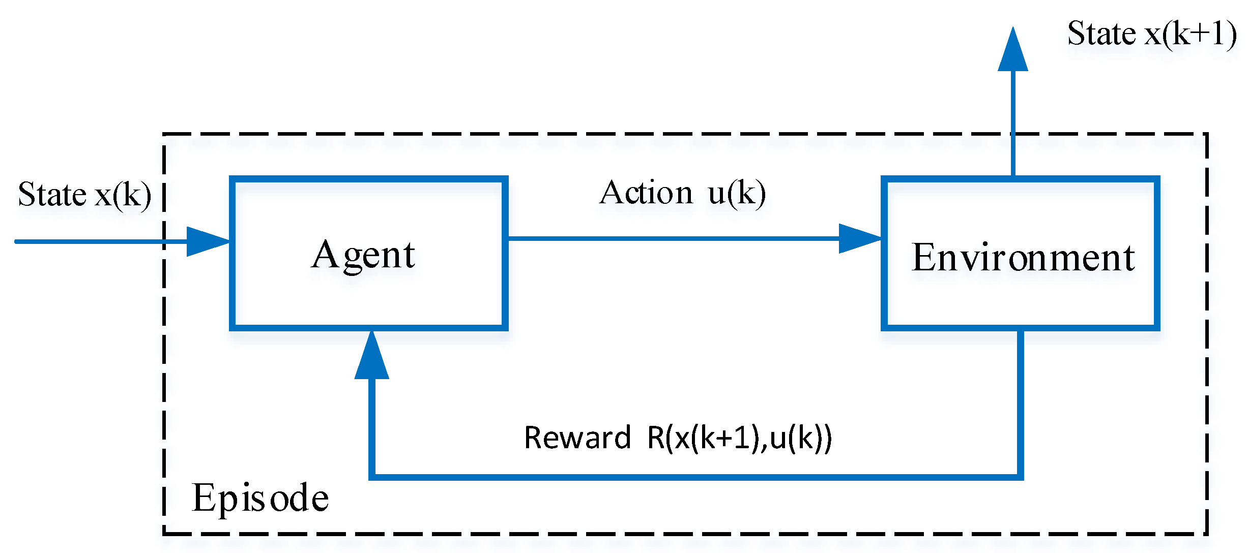
Reinforcement learning (RL), motivated by psychology, statistics, neuroscience, and computer science, is about learning from interaction how to behave in order to achieve a design goal [32,33,34]. It will get rid of the limitation of training samples by learning directly from the raw data online. Through the learning process, an optimal action will be achieved to respond to the states. By sensing the current states, the RL does not need the assumption of prior distribution of noise. By episodes training, the action will overcome the overfitting difficulty and become robust due to eliminating the disturbance gradually. If the parameters were taken as the actions, they would be determined by reinforcement learning without thinking about the assumptions and disadvantages of the methods. In the case of a forging machine, it is a feasible approach to find the optimal values of the model parameters in a new condition under disturbances. There are some mature algorithms in the RL family, such as Q-learning [35], actor–critic [36], and deep reinforcement learning [37]. In this study, the Q-learning algorithm is proposed to determine the model parameters under the working condition due to its simplicity. The contributions of this paper can be summarized as follows:

(1)

The parameters are identified only based on the information of one period, which is promising for online control.

(2)

The values of parameters are determined directly by raw data without any assumptions of noisy characteristics.

(3)

The parameters have strong stability through a number of training episodes, which resists the bad influence of disturbance of unknown law.

The rest of this paper is organized as follows. Section 2 gives the model of pressing-down in forging machine that shows the state variables and the parameters. Section 3 describes the RL’s procedure and releases the proposed approach. In Section 4, the model parameters are elaborated by the proposed approach and comparisons are made with two classical methods. Finally, conclusions are drawn in Section 5.

2. The Model of the Pressing-Down in Forging Machine

A semisolid metallic confectioning constant-speed isothermal forging is an important forging technique especially for light-weight alloy confectioning in the aerospace industry. The typical structure of the forging machine is illustrated in Figure 1, and the model has been built in our previous work [38]. It is repeated here for integrity.

The function of the forging machine in pressing-down phase is affected by the oil pipe-line, the proportional servo valve, and the hydraulic cylinder with abandoning the auxiliary attachments.

2.1. The Oil Pipe-Line

The pressing speed in the pressing-down phase is always slow to meet the craft needs, so the oil works in the state of filament flow. Taking a pipe oil column as an object, the pressure balance equation is in the form of Formula (1).

$$\rho S_{1}l\frac{d\left(q_1/S_1\right)}{dt}=\left(p_1-p_s\right)S_1-\frac{128\mu l}{\pi d^2}{q}_1{S}_1$$

(1)

Let $\mathrm{R}=\frac{32\mu }{\rho }$, so Formula (1) becomes

$$\frac{1}{S_1}\frac{d{q}_1}{dt}=\frac{p_1-p_s}{\rho l}+\frac{R}{S_1}{q}_1$$

(2)

The difference between input volume and output volume is equal to the sum volume of oil compress and pipe swelling. So the oil continuity equation is

$$q_2-q_1=\frac{S_{1}l}{K}\frac{d\left(p_1-p_s\right)}{dt}$$

(3)

where $q_1$ and $q_2$ are the oil flow in pipe and the output oil flow of proportional servo valve, $p_1$ and $p_s$ are the input pressure of proportional servo valve and the pressure of a constant rate pump output, $S_1$ and $l$ are the sectional area of pipe and the length of oil pipe, and $K$ is the young’s modulus of oil equal volume.

2.2. Proportional Servo Valve

The proportional servo valve performs between the servo valve and the proportional valve. It eliminates the dead band by the way of fluid forerunner. The proportional servo valve is widely applied in the ultra-low-speed hydraulic machine to control the oil flow to the hydraulic cylinder. The proportional servo valve is described as

$$\frac{1}{{\omega }_n^2}\frac{d^2{q}_2}{d{t}^2}+\frac{2\xi }{{\omega }_n}\frac{d{q}_2}{dt}+q_2=K_{q}A$$

(4)

where $\xi$ amd ${\omega }_n$ are the damping rate and the inherent frequency of propositional servo valve, respectively, $K_q=K_n\sqrt{\frac{p_1-p_2}{\Delta p_n}}$ is used to compensate the error between the practical pressure and criterion pressure, and $A$ is the opening of proportional servo valve.

2.3. The Hydraulic Cylinder

The pipe-line between proportional servo valve and the hydraulic cylinder is omitted due to its short distance. The oil continuity equation of hydraulic cylinder is the form of

$$q_2=S_{2}v+{\lambda }_c{p}_2+\frac{V_c}{K}\frac{d{p}_2}{dt}$$

(5)

where $S_2$ is the plunger’s sectional area of exporting cavity of hydraulic cylinder, $v$ is the moving speed of plunger, ${\lambda }_c$ is the leak coefficient of hydraulic cylinder,$p_2$ is the output pressure of proportional servo valve, and $V_c$ is the oil volume of upper cavity of hydraulic cylinder, $V_c=V_0+vS$.

The dynamic equation of plunger is obtained according to the force analysis with the form of

$$p_2{S}_2+mg=m\frac{dv}{dt}+Bv+F+p_3{S}_2$$

(6)

where $m$ is the mass of slider block, $g$ is the acceleration of gravity, $B$ is the viscous damping coefficient, $F$ is the load resistance, and $p_3$ is the holding pressure of slide block. According to the design of forging machine, the holding power of slide block is equal to the gravity of slide block:

$$p_3{S}_2=mg$$

(7)

The Formula (6) is simplified to Formula (8) by substituting Formula (7) for Formula (6):

$$p_2{S}_2=m\frac{dv}{dt}+Bv+F$$

(8)

2.4. The Model of the System as a Whole

Let $x_1=q_1,x_2=p_1-p_s,x_3=\frac{d{q}_2}{dt},x_4=q_2,x_5=p_2,\mathrm{and}{x}_6=v.$ By integrating the subsystems together, the global forging machine model can be described in the state–space form

$$\dot{x}=f\left(x\right)+g\left(x\right)u$$

(9)

where $x={\left[x_1,x_2,x_3,x_4,x_5,x_6\right]}^T$, $u=A$,

$$\begin{array}{c}f\left(x\right)=\\ \left[\begin{array}{cccccc}\frac{R}{S_1}& \frac{S_1}{\rho l}& 0& 0& 0& 0\\ -\frac{K}{S_{1}l}& 0& 0& \frac{K}{S_{1}l}& 0& 0\\ 0& 0& 0& 1& 0& 0\\ 0& 0& -2\xi {\omega }_n& -{\omega }_n{}^2& 0& 0\\ 0& 0& 0& \frac{K}{V_c}& -\frac{K{\lambda }_c}{V_c}& -\frac{K{S}_2}{V_c}\\ 0& 0& 0& 0& \frac{S_2}{m}& -\frac{B}{m}\end{array}\right]\left[\begin{array}{c}{x}_1\\ x_2\\ x_3\\ x_4\\ x_5\\ x_6\end{array}\right],\\ \hspace{1em}\hspace{1em}\hspace{1em}g={[0,0,0,{\omega }_n{}^2{K}_n\sqrt{\frac{x_2-x_5+P_s}{\Delta p_n}},0,-\frac{F}{B}]}^T\end{array}$$

Remark 1.

In the model, most parameters such as the length, the sectional area of oil pipe, the mass of slider block, and the rated flow gain can be valued according to the design. The values of parameters that are influenced by the surrounding or working conditions will result in the inaccuracy of model.

3. The Proposed Method

3.1. Reinforcement Learning

The basic frame of reinforcement learning is shown in Figure 2. At each time step k, the agent makes observations $x\left(k\right)\in X$ and takes action $u\left(k\right)\in U$, and receives reward $R\left(x\left(k+1\right),x\left(k\right), u\left(k\right)\right)\in ℝ$.

The expected return that is received in the long run is described using the state–action value function $\mathrm{V}\left(x, u\right)$, under the condition of first taking an arbitrary action $u\in U$ from a certain state $x\in {\rm X}$ and subsequently acting according to a certain control series π. So the value function ${\mathrm{V}}_{\mathsf{\pi }}\left(x\left(k\right), u\left(k\right)\right)$ at time $k$ is defined as

$${\mathrm{V}}_{\mathsf{\pi }}\left(x\left(k\right), u\left(k\right)\right)={\displaystyle \sum }_{t=k}^{\infty }\gamma R\left(x\left(k+1\right),x\left(t\right), u\left(t\right)\right)$$

(10)

where $\gamma \in \left[0,1\right]$ is the discount factor.

The value function ${\mathrm{V}}_{\mathsf{\pi }}\left(x\left(k+1\right), u\left(k\right)\right)$ at time k + 1 is defined as

$${\mathrm{V}}_{\mathsf{\pi }}\left(x\left(k+1\right), u\left(k\right)\right)={\displaystyle \sum }_{t=k+1}^{\infty }\gamma R\left(x\left(t+1\right),x\left(t\right), u\left(t\right)\right)$$

(11)

According to the theory of dynamic programming

$${\mathrm{V}}_{\mathsf{\pi }}\left(x\left(k\right), u\left(k\right)\right)=R\left(x\left(k+1\right),x\left(k\right), u\left(k\right)\right)+{\mathrm{V}}_{\mathsf{\pi }}\left(x\left(k+1\right), u\left(k\right)\right)$$

(12)

Unfortunately, the value function ${\mathrm{V}}_{\mathsf{\pi }}\left(x\left(k\right), u\left(k\right)\right)$ and ${\mathrm{V}}_{\mathsf{\pi }}\left(x\left(k+1\right), u\left(k\right)\right)$ is not obtained because no one knows the rewards after time $k+1$. To remove this obstacle, the Q-function is designed with $Q\left(x\left(k\right),u\left(k\right)\right)$ and $Q\left(x\left(k+1\right),u\left(k\right)\right)$ replacing ${\mathrm{V}}_{\mathsf{\pi }}\left(x\left(k\right), u\left(k\right)\right)$ and ${\mathrm{V}}_{\mathsf{\pi }}\left(x\left(k+1\right), u\left(k\right)\right),$ respectively

Let

$$\delta =R\left(x\left(k+1\right),x\left(k\right), u\left(k\right)\right)+\gamma Q\left(x\left(k+1\right),u\left(k\right)\right)-Q\left(x\left(k\right),u\left(k\right)\right)$$

(13)

The $u\left(k\right)$ will be optimized by a process of seeking $\delta$ approach to zero.

As an important member of reinforcement learning family, the basic step of Q-algorithm is carried out as Procedure 1 [30].

Procedure 1.

 

Initialize$Q\left(x\left(k\right),u\left(k\right)\right)$arbitrarily

Repeat (for each episode)

Initialize$x\left(k\right)$

Repeat (for each step of episode)

Choose$u\left(k\right)$from$x\left(k\right)$using policy derived from$Q$(e.g.,$\epsilon -greedy$)

Take action$u\left(k\right)$, observe$R\left(k\right), x\left(k+1\right)$

$Q\left(x\left(k\right),u\left(k\right)\right)\leftarrow Q\left(x\left(k\right),u\left(k\right)\right)+\alpha \left[R\left(k\right)+\gamma ma{x}_{u\left(k+1\right)}Q\left(x\left(k+1\right),u\left(k+1\right)\right)-Q\left(x\left(k\right),u\left(k\right)\right)\right]$

$x\left(k\right)\leftarrow x\left(k+1\right)$until$x\left(k\right)$is terminal.

Remark 2.

There is only state information in Procedure 1. One can obtain the optimal action online by using two states, $x\left(k\right)$ and $x\left(k+1\right),$ in the process of maximizing the value function. By this way, it makes an online control become possible because this approach gives up the requirement of sliding window length.

3.2. The Proposed Approach

The scheme of proposed approach is shown in Figure 3.

A model that consists of undetermined parameter $p$ ($p\in R^m$) is paralleled to the forging machine under the controller. The state variables of model are recorded as $x\left(k\right)$ and $x\left(k+1\right)$ at sampling $k$ and $k+1,$ which are connected by a delay link ${\mathrm{z}}^{-1}$. The undetermined parameter $p$ is regarded as the action of Q-algorithm. Therefore, the Q-algorithm following Procedure 1 is applied to determine the parameter $p$ based on $x\left(k\right)$ and $x\left(k+1\right)$ and finally, the optimal parameter $p^{*}$ will be obtained when it is convergent.

To explicate Q-algorithm for the acquisition of model parameters, the key concepts of the proposed Q-algorithm are illustrated as follows.

(i).

Action space, reward, and value function

The action space is made up of the undetermined parameter $p$. The values of parameter are usually inconsistent with the working condition, which will disturb with model accuracy. A goal is to determine their values responding to the surroundings.

The forging machine’s velocity is designated a constant pressing speed or a given curve of speed during a certain temperature range according to the properties of forging materials, so the reward $\mathrm{R}\left(k\right)$ is selected as the reciprocal of change for absolution error between the measured speed and the set speed at adjacent sampling times $k$ and $k+1$

$$\mathrm{R}\left(k\right)=\frac{1}{\left|\left|v\left(k\right)-v_{set}\left(k\right)\right|-\left|v\left(k+1\right)-v_{set}\left(k+1\right)\right|\right|}$$

(14)

where $v\left(k\right)$ and $v_{set}\left(k\right)$ are the measured speed and the preset speed at sample $k$; $v\left(k+1\right)$ and $v_{set}\left(k+1\right)$ are the measured speed and the preset speed at sample $k+1$. Here, using $v$ instead of $x_6$ that is the sixth component of state vector $x$ is only to stress the physics meaning.

Let $s=\left[x;u\right]$ so the value functions $\mathrm{V}\left(s\left(k\right),p\left(k\right)\right)$ and $\mathrm{V}\left(s\left(k+1\right),p\left(k+1\right)\right)$ from samples $k$ and $k+1$ are defined by Formulas (15) and (16)

$$\mathrm{V}\left(s\left(k\right),p\left(k\right)\right)={\displaystyle \sum }_{i=k}^{\infty }\mathrm{R}\left(i\right)$$

(15)

$$\mathrm{V}\left(s\left(k+1\right),p\left(k+1\right)\right)={\displaystyle \sum }_{i=k+1}^{\infty }\mathrm{R}\left(i\right)$$

(16)

(ii).

Q-function

The value functions $\mathrm{V}\left(s\left(k\right),p\left(k\right)\right)$ and $\mathrm{V}\left(s\left(k+1\right),p\left(k+1\right)\right)$ are replaced by Q-function according to the Q-algorithm because the value functions are not obtained due to the unknown rewards after sample $k$. The early Q-function that is applied for the discrete space is presented as a look-up table of states row and actions column. When the states or actions are continuous, their discretization will lead to the curse of dimensionality by generating an exponentially increasing complexity of algorithm and insufficient storage. Therefore, the parameterized function is proposed to fit the Q-function with the form

$$\mathrm{Q}\left(s\left(k\right),p\left(k\right)\right)=f\left(s\left(k\right),p\left(k\right),\theta \right)$$

(17)

where $f$ and $\theta$ are a parameterized mapping and the parameters, respectively. Let $s=\left[s;p\right]$, an approximator is used to substitute for the unknown parameterized mapping, and there is

$$\hat{\mathrm{Q}}\left(s\right)={\displaystyle \sum }_{i=1}^{\mathrm{n}}{\varphi }_i\left(s\right){\theta }_i$$

(18)

where ${\varphi }_i\left(s,a\right)$ is usually selected as Gauss radial kernel function due to its simplicity, whose form is

$${\varphi }_i\left(s\right)=e^{-\frac{\Vert s-s_i{\Vert }^2}{2{\sigma }_i^2}}$$

(19)

in which $s_i$ is the central coordinates of $i$-th radial kernel function and ${\sigma }_i$ is the width of $i$-th radial kernel function.

(iii).

Exploitation and exploration

There are two ways to determine the action in RL. The exploitation is used to get the best action from the Q-function that is based on the reward received. The exploration is used to escape the local optimization of exploitation by randomly giving the action. As a compromise of exploitation and exploration, the $\epsilon -$ greedy algorithm is proposed to evolve the action. The agent selects the action that maximizes the Q-value function according to the probability $\epsilon$ that is usually a large probability event. In addition, it selects the action randomly according to the probability of $1-\epsilon$ from the action space, which makes sure the action exploration is within the unknown area. The form of $\epsilon -$ greedy algorithm is

$$p\left(k+1\right)=\{\begin{array}{c}\underset{p\left(k\right)}{argmax}Q\left(s\left(k\right),p\left(k\right),\theta \right), Pr<\epsilon \\ rand\left(U\right), Pr\le 1-\epsilon \end{array}$$

(20)

where $p\left(k\right)$ and $p\left(k+1\right)$ are the acquisition parameter at $k$ and $k+1,$ respectively, $Pr$ is the probability of select action, and $U$ is the action set.

(iv).

The Process of Method

The proposed algorithm is summarized as Procedure 2. In this procedure, the input states are $x\left(k\right)$, $u\left(k\right)$ and $x\left(k+1\right),$ whose physical meanings are shown in Section 2, and the output parameter is $p$.

Procedure 2.

 

Step 1: Give a state$x\left(k\right)$and the control$u\left(k\right)$and then construct$s$according to$s=\left[x; u \right]$

Step 2: Select parameters$p\left(k\right)$randomly.

Step 3: Observe the next state$x\left(k+1\right)$

Step 4: Receive immediate reward$R\left(k\right)$according to Formula (14)

Step 5: select$p\left(k+1\right)$according to Formula (20)

Setp6: Compute$Q\left(s\left(k\right),p\left(k\right),\theta \right)$and$Q\left(s\left(k+1\right),p\left(k+1\right),\theta \right)$according to the Formulas (18) based on the model of Formula (9)

Step7: Compute the time series error$\delta \left(k\right)$according to

    $\delta =R\left(k\right)+\gamma Q\left(s\left(k+1\right),p\left(k+1\right),\theta \right)-Q\left(s\left(k\right),p\left(k\right),\theta \right)$

Step 8: Update$Q\left(s\left(k\right),p\left(k\right),\theta \right)$according to

     $Q\left(s\left(k\right),p\left(k\right),\theta \right)\leftarrow Q\left(s\left(k\right),p\left(k\right),\theta \right)+\alpha \delta$

Step9:$x\left(k\right)\leftarrow x\left(k+1\right),u\left(k\right)\leftarrow u\left(k+1\right)$and$p\left(k\right)\leftarrow p\left(k+1\right)$

Step 10: Repeat steps 3 to 9 until it is convergent. The output$p$is the convergent$p\left(k\right)$in which$p\left(k\right)=p\left(k+1\right)=p$.

(v).

Convergence

The convergence of Q-algorithm can be found in [35,36].

4. Case Studies

The forging machine usually keeps a good state at the early life stage. In this stage, the values of parameters after a fine machine debugging always coincide with the design condition, except for the viscous damping coefficient $B$ because it is prone to be influenced by the temperature and working condition. With time elapsing, the leakage becomes the main uncertainty of the forging machine. A little leakage is permitted for the forging machine if the leakage does not affect the work process. Nevertheless, the forging machine needs to be repaired if there appears much leakage. Therefore, we chose the viscous damping coefficient $B$ and leakage coefficient ${\lambda }_c$ as the identification parameters. These two parameters are unmeasurable, which make their values unverifiable in practice. As a result, we conducted a simulation to verify the proposed method.

4.1. Data Source

The state space model of (9) was used to simulate a forging machine. The values of model parameters are shown in

Table 1. The parameters values under the design condition.

$\mathit{\xi }$	${\mathit{\omega }}_{\mathit{n}}$	$\mathit{R}$	${\mathit{S}}_1$	$\mathit{\rho }$	$\mathit{l}$	m	$\mathit{K}$	${\mathit{S}}_2$	${\mathit{V}}_0$	${\mathit{K}}_{\mathit{n}}$	${\mathit{P}}_{\mathit{s}}$	$\Delta {\mathit{p}}_{\mathit{n}}$
			${\mathrm{m}}^2$	kg/${\mathrm{m}}^3$	m	kg		${\mathrm{m}}^2$	${\mathrm{m}}^2$		Mpa	pa
0.7	70	0.0064	0.0138	870	7	1 × 104	1 × 1010	0.02463	4.9 × 10−3	2 × 10−4	12	3.5 × 106

according to the design condition.

A controller is necessary for a forging machine to guarantee the quality of pressing process, therefore, a PID controller was used to simulate this situation. We chose a PID controller because here we focus on verifying our proposed method rather than discussing the control method. The PID controller is enough to provide the states and control for the proposed approach. The data series were generated by solving the model (9) with ODE45 that applies the fourth-order Runge Kutta algorithm to provide the candidate solution and the fifth-order Runge Kutta algorithm to control errors. These continuous sequences provided the data source by adding two kinds of noise with uniform distribution or Gaussian distribution as a simulation of real data. The set speed was changed from 0.02 to 0.08 that is consistent with the requirement of a typical pressing process. A typical control process that includes a transition process and a stable process is shown in Figure 4.

The subsequent simulation was carried out at the platform of MatlabR2011b with the computer of Intel^® Core™ 2 Duo CPU E7300 @2.66GHz 2.67GHz.

4.2. Acquisition of the Viscous Damping Coefficient

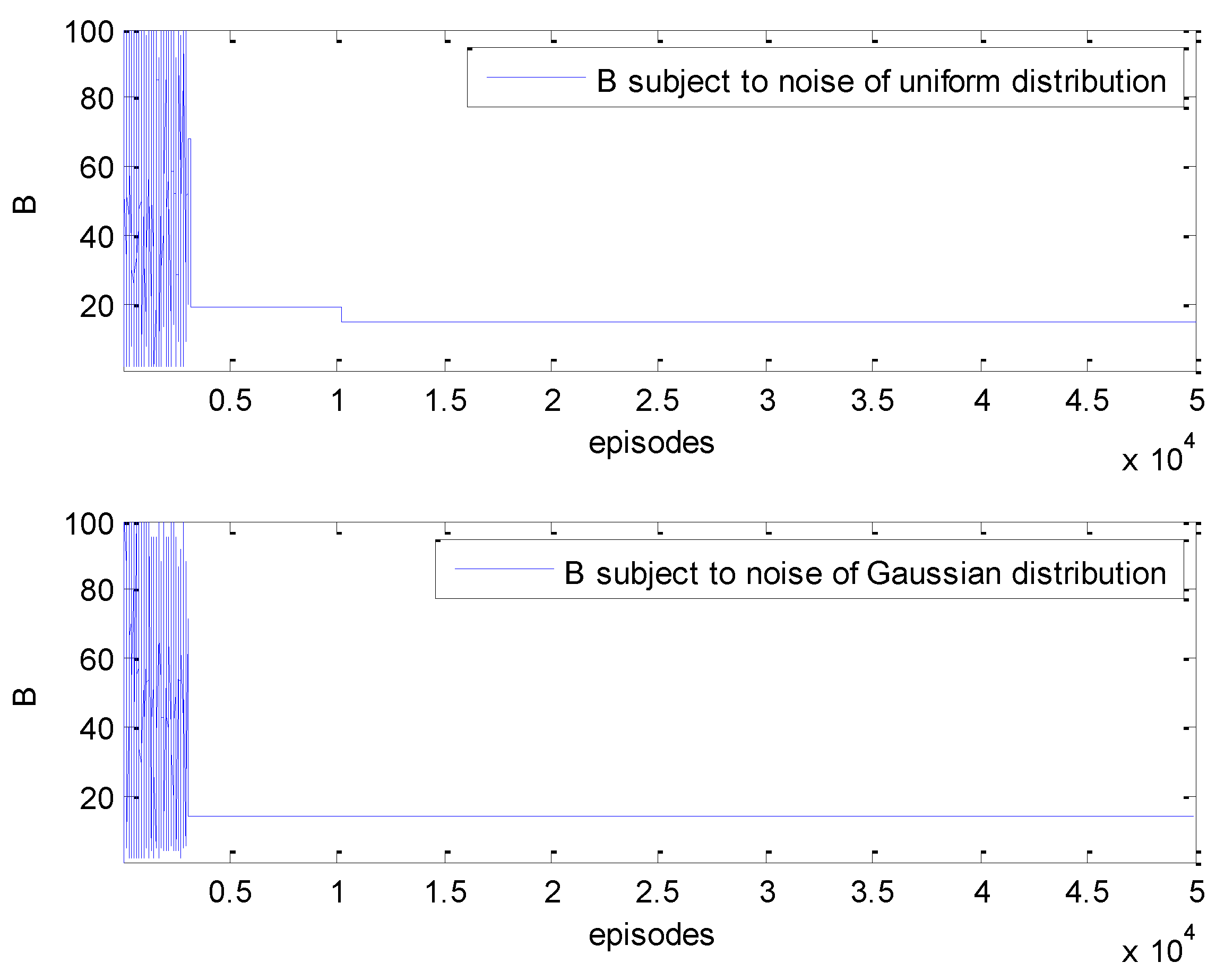
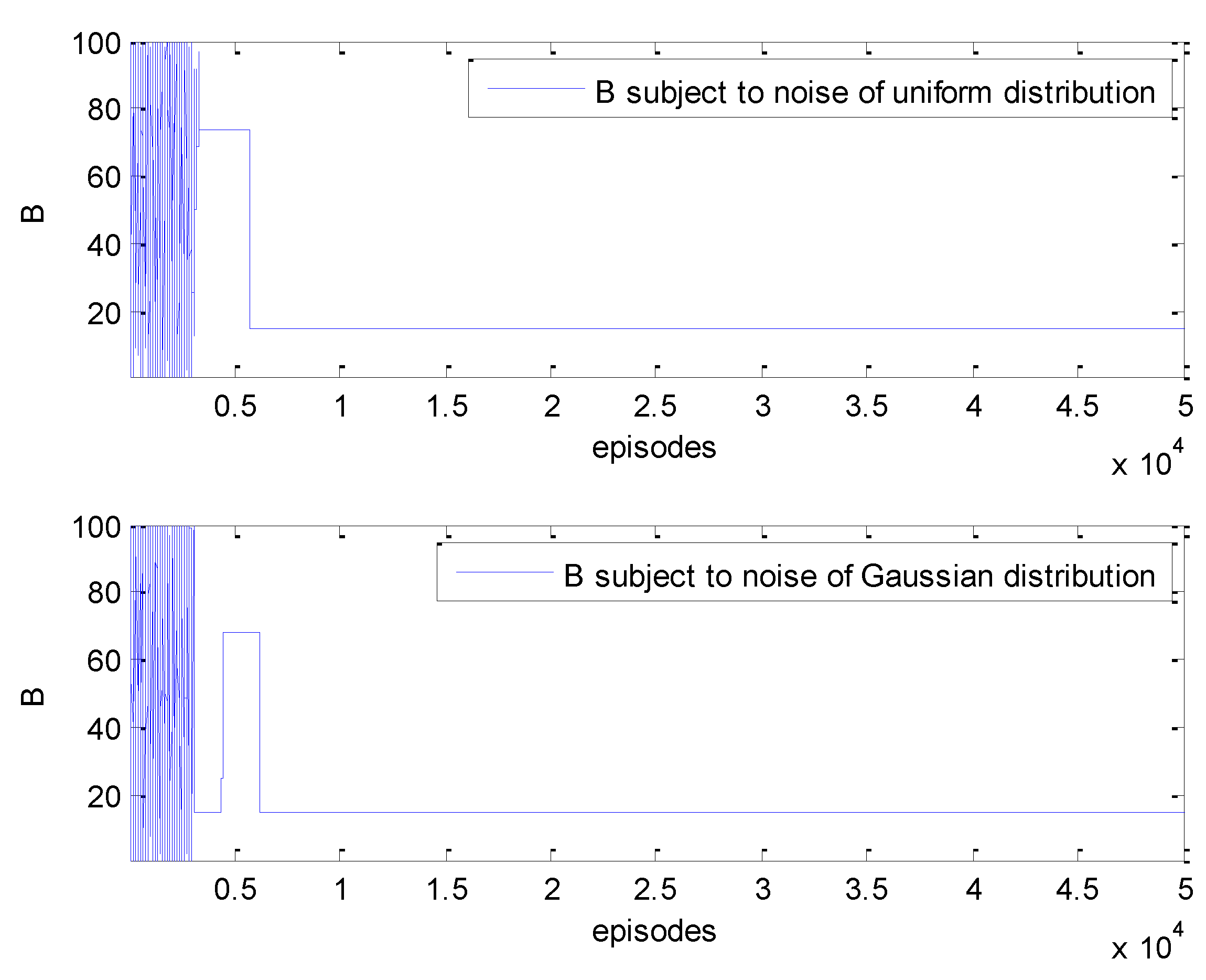
According to experiments, the viscous damping coefficient $B$ is usually during 10–30 for this model. As a result, the value of 15 was chosen as the predetermined value and targeted by the proposed approach according to Procedure 2. The episodes training process is shown in Figure 5, where the subgraph above is with the noises of the uniform distributions and the subgraph below is with the noises of the Gaussian distributions. It is generally believed that the training time is related to the nature of the object and the computer performance. In order to avoid the time difference caused by different computer performance, we used the number of the episodes as an index of training time.

Figure 5 shows there is a trial process at the beginning of training because there is no priori information on $B$. After a trial of about 3000 episodes, the best historical value of $B$ that indicates 20 for the above subgraph and 15.0626 for the below subgraph appears during the process of seeking the best reward. After about 10,000 episodes, a better value of 14.5000 occurs for the above subgraph. In contrast, a value of 15.0626 for the below subgraph is unchanged until the episodes terminate.

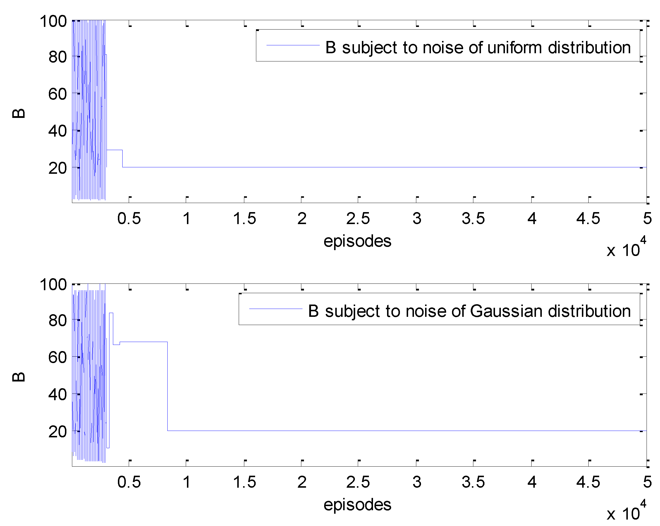
The viscous damping coefficient $B$ was changed from 15 to 20 to test the proposed method. The episodes training process is shown under a uniform distribution (the above subgraph) and under a Gaussian distribution (the below subgraph). Figure 6 shows the training episodes process similar to Figure 5. It is also seen that the trial process of Figure 6 lasts about 3000 episodes.

In order to show the accuracy of parameter acquisition, the relative error $\delta$ between the estimated value $\widehat{B}$ and the predetermined value $B_r$ is defined as a form of

$$\delta =\left(\widehat{B}-B_r\right)/B_r$$

(21)

and the results are shown in

Table 2. The results of viscous damping coefficient without leakage.

Predetermined Value	Noise Distribution	Acquisition	Relative Error
15	Uniform	15.0626	0.4%
15	Gaussian	14.5000	3.33%
20	Uniform	19.0000	5%
20	Gaussian	19.0000	5%

It is seen from Figure 5 and Figure 6 that the excellent results with relative errors no greater than 5% were obtained in the cases of noises with different distributions.

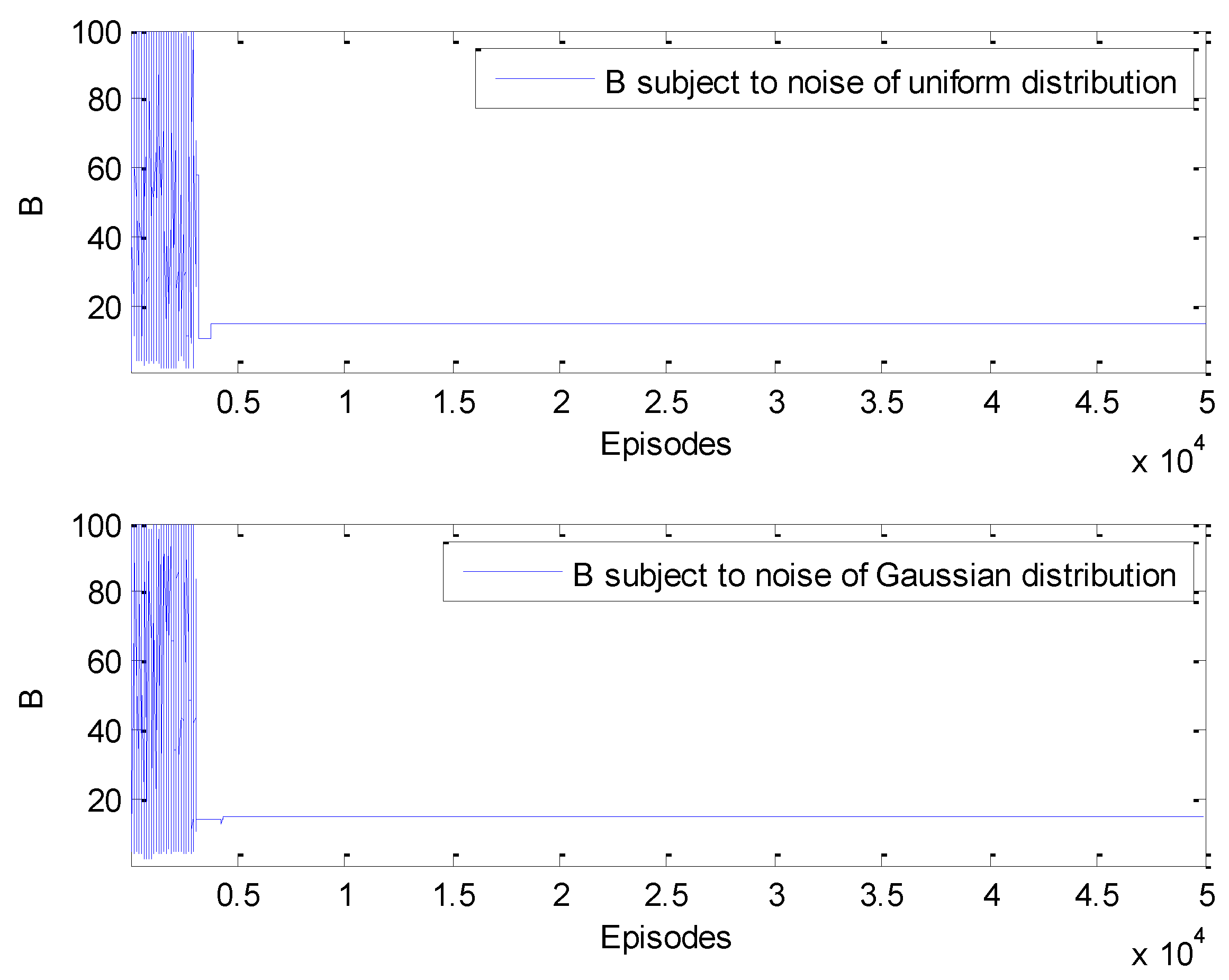
Further tests under the condition of oil leakage were done to verify the effectiveness of the proposed approach. For a forging machine, the leakage is prone to go into saturation and is limited to a small value, so the leakage coefficients ${\lambda }_c$ were assumed as a constant 0.01 and 0.02. The episodes training processes are shown in Figure 7, Figure 8, Figure 9 and Figure 10. Figure 7 and Figure 8 present the training processes of acquiring the viscous damping coefficient with a goal of 15 and of 20, respectively, under the leakage coefficient of 0.01. Figure 9 and Figure 10 present the training processes of acquiring the viscous damping coefficient with a goal of 15 and of 20, respectively, under the leakage coefficient of 0.02. These figures show the proposed approach will be convergent after episodes training processes, and the final results are listed in

Table 3. The results of viscous damping coefficient under leakage.

$\mathbf{Leakage}\mathbf{Coefficient}{\mathit{\lambda }}_{\mathit{c}}$	Noise Distribution	Acquisition B	Predetermined Value B	Relative Error
0.01	Uniform	15.0000	15	0%
0.01	Gaussian	15.2500	15	1.67%
0.01	Uniform	20.0000	20	0%
0.01	Gaussian	20.0000	20	0%
0.02	Uniform	15.0000	15	0%
0.02	Gaussian	15.0000	15	0%
0.02	Uniform	20.0000	20	0%
0.02	Gaussian	19.9375	20	0.31%

. Table 3 shows the viscous damping coefficient will approach the predetermined value $B_r$ under different coefficients or different noise distributions, showing a maximal relative error less than 2%. For training time, there are some differences for different parameters, such as about 6000 episodes in Figure 7, about 4000 episodes in Figure 9, and about 3000 episodes in Figure 10. Sometimes the different distributions also have an effect on the training speed, which is shown in Figure 8.

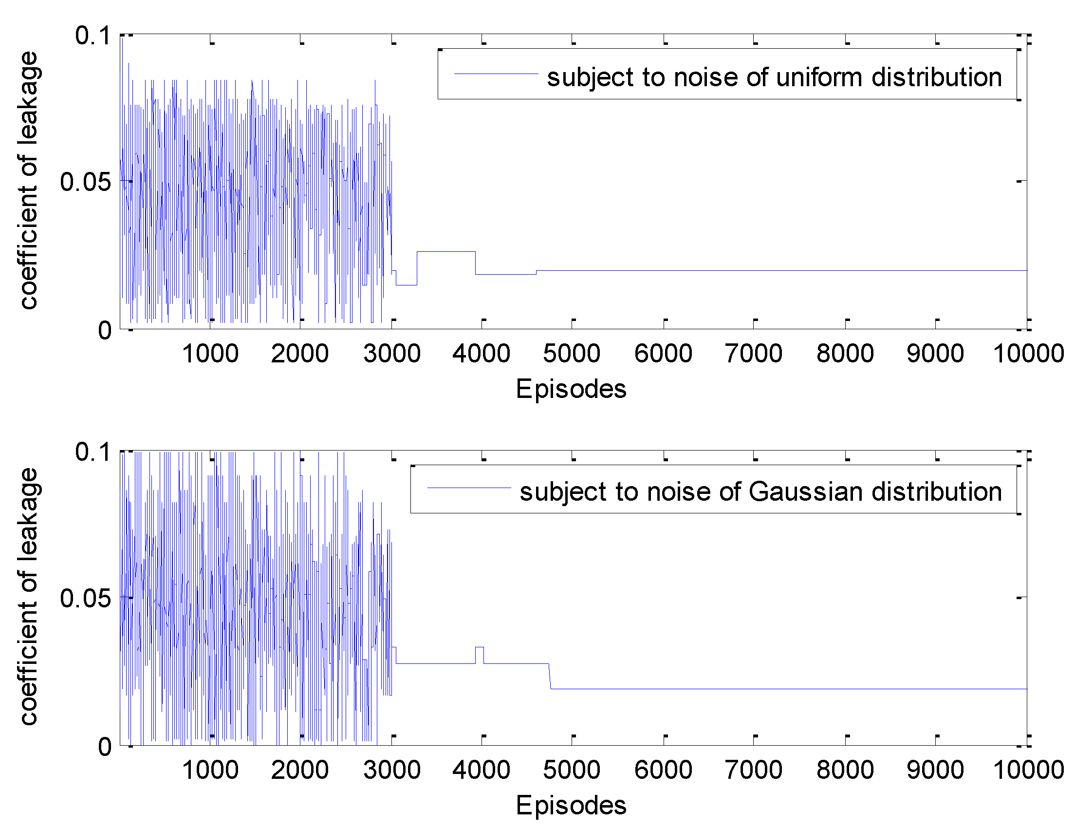
4.3. Acquisition of the Leakage Coefficient

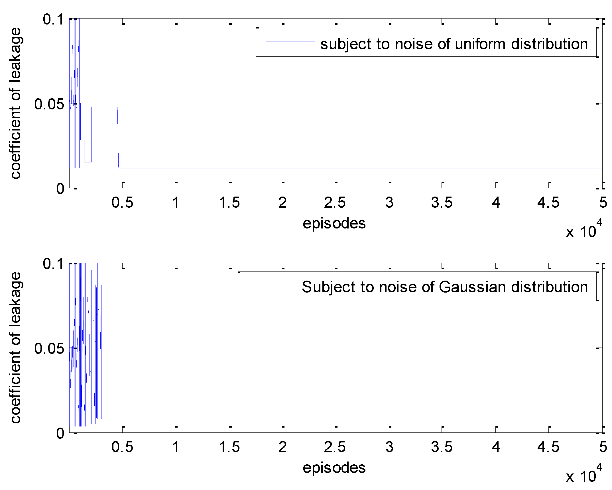
The leakage that is marked with leakage coefficient ${\lambda }_c$ in the model will become the main uncertainty along with the lapsing time of forging machine. The leakage coefficient was predetermined as a constant 0.01 and 0.02. The learning processes with uniform distribution and with Gaussian distribution are shown in Figure 11 and Figure 12, respectively. As for training time, it is affected by different distributions in Figure 11 and about 5000 episodes in Figure 12.

The values of leakage coefficient ${\widehat{\lambda }}_c$ are acquired when the curve becomes stable. Here, the absolute error $E$ with the definition of

$$E=\left|{\lambda }_c-{\widehat{\lambda }}_c\right|$$

(22)

was used to replace the former relative error because the value of leakage coefficient is too small as the denominator of Formula (22), which is prone to an inappropriate relative error. The results are listed in

Table 4. The results of leakage coefficient.

Predetermined Value	Noise Distribution	Acquisition	Absolute Error
0.01	Uniform	0.0114	0.0014
0.01	Gaussian	0.0075	0.0015
0.02	Uniform	0.0200	0
0.02	Gaussian	0.0187	0.0013

. Table 4 shows the absolute errors are not more than 0.0015 in the cases of noisy with different distributions.

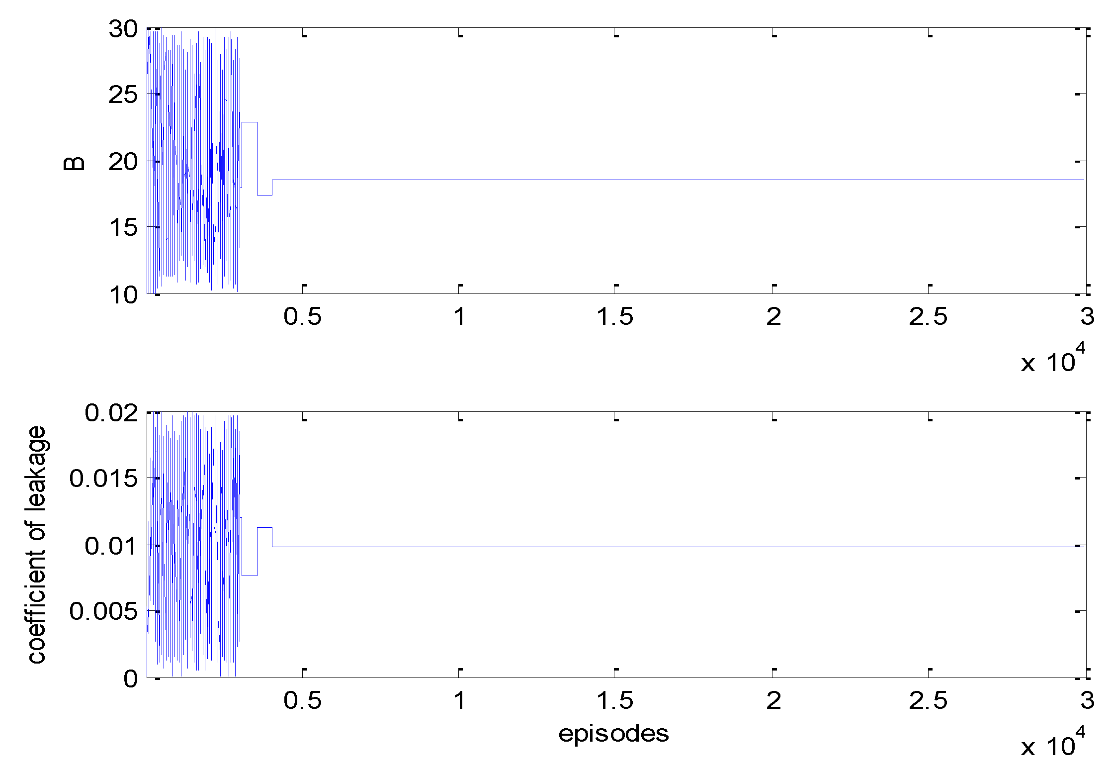
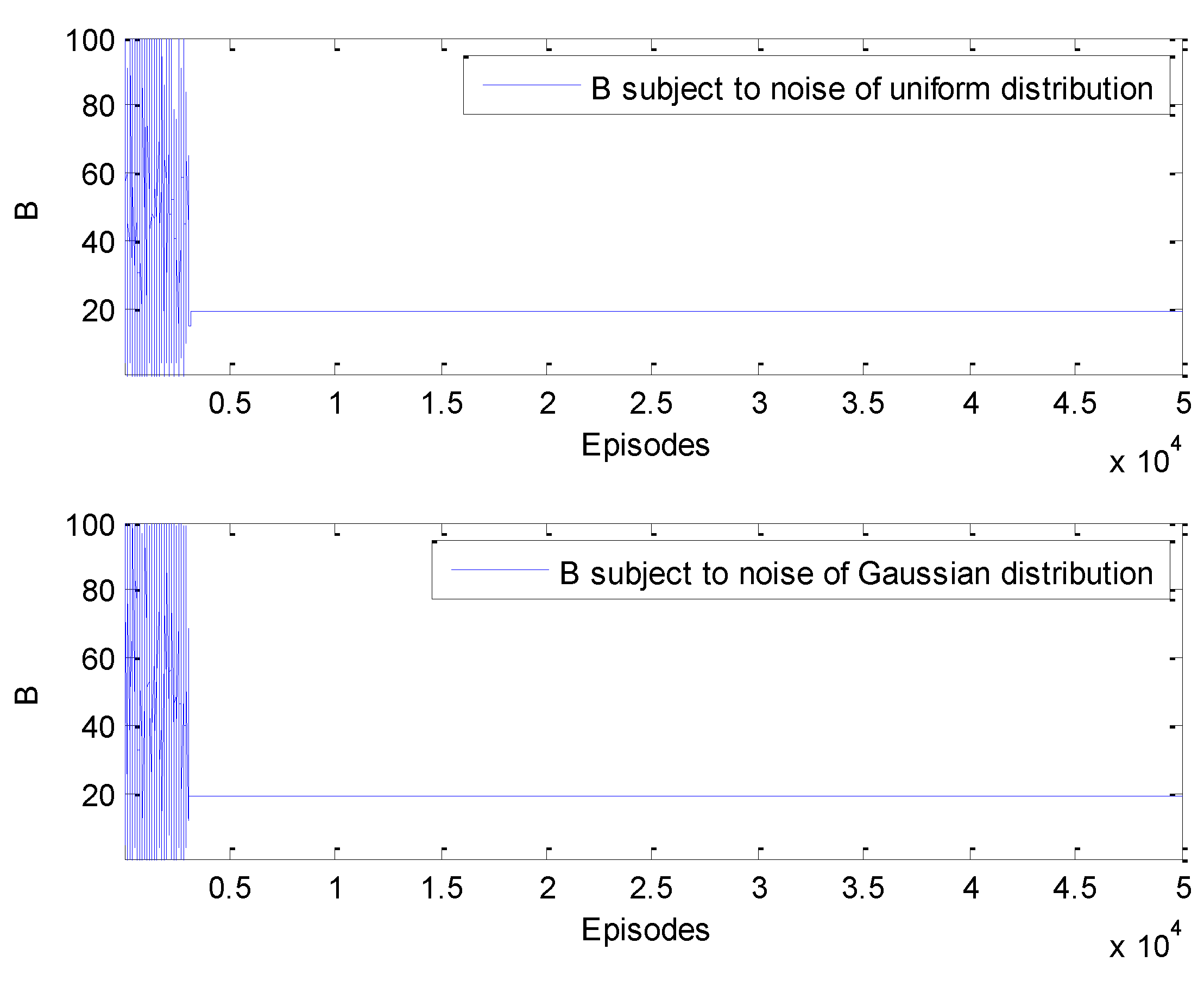
4.4. Acquisition of the Viscous Damping Coefficient and the Leakage Coefficient

In order to test higher dimensionality of parameters, an experiment on acquiring concurrently the viscous damping coefficient and the leakage coefficient was done. The parameters of B and ${\lambda }_c$ were predetermined as 18 and 0.01, respectively. The learning processes with uniform distribution and with Gaussian distribution are shown in Figure 13 and Figure 14, respectively, and the results are shown in

Table 5. The results of the viscous damping coefficient and the leakage coefficient concurrently.

Noise Distribution	Parameters	Predetermined Value	Acquisition
Uniform	$\mathrm{Viscous}\mathrm{damping}\mathrm{coefficient}B$	18	18.0488
	$\mathrm{Leakage}\mathrm{coefficient}{\lambda }_c$	0.01	0.0102
Gaussian	$\mathrm{Viscous}\mathrm{damping}\mathrm{coefficient}B$	18	18.4141
	$\mathrm{Leakage}\mathrm{coefficient}{\lambda }_c$	0.01	0.0098

, which shows both parameters can reach a good estimation concurrently in the cases of noisy conditions. Here, all the training times are less than 5000 episodes.

4.5. Comparison with Other Methods

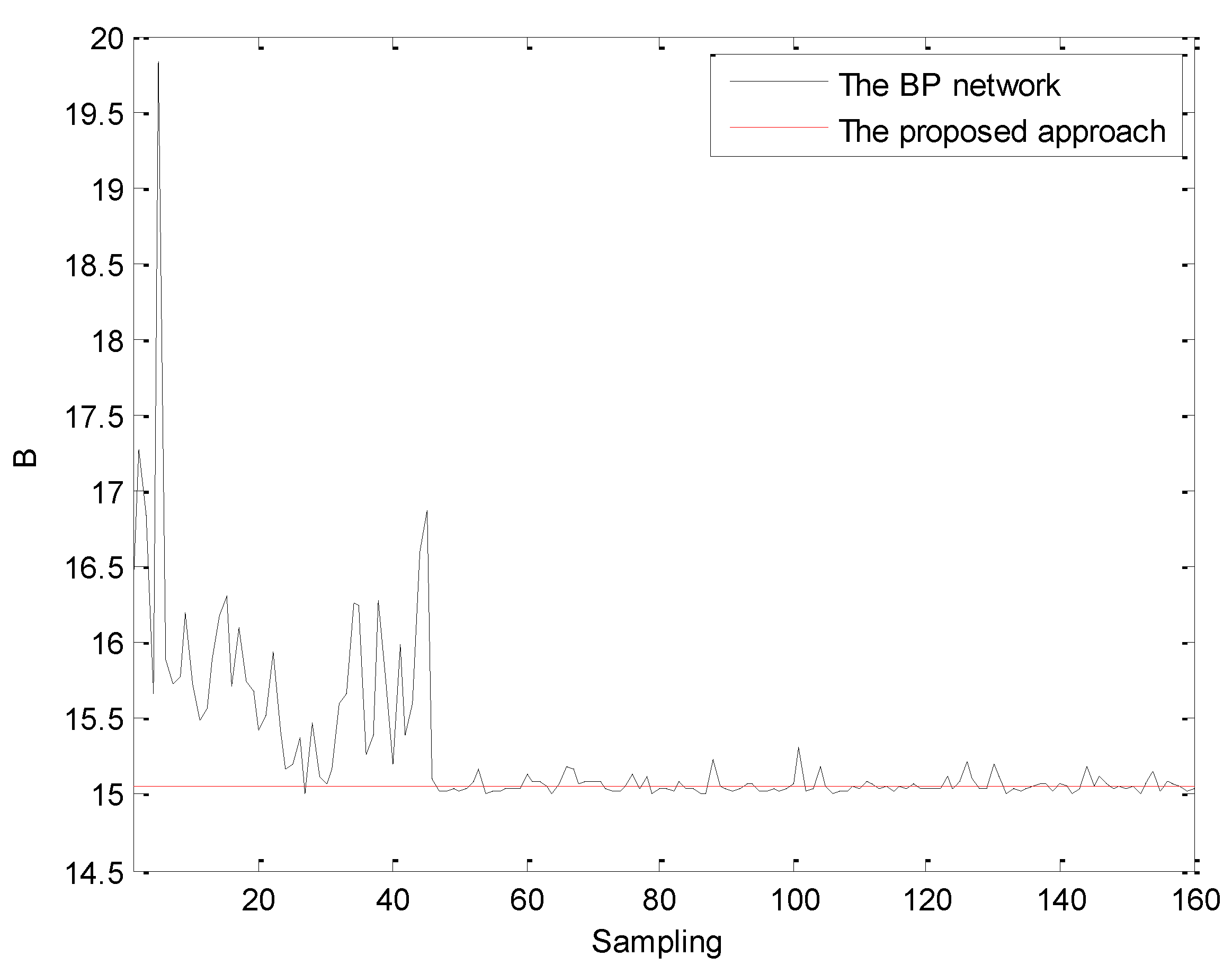
A famous BP network approach and the sliding window correlation methods were chosen as a comparison of the proposed approach. The data series with 160 samples that was produced by the model with a controller was considered as the data source to determine the parameters. This data series includes a transient process of 50 and a stable process of 110 based on the viscous damping coefficient $B$ of 15.

As we know, the BP network has a strong nonlinear approximation ability and an excellent estimation of recursion problem, which needs the length of input time series to match the order of the system. Here, we focused on identifying the parameter of viscous damping coefficient $B$ just in one period. After several attempts, the BP network was chosen as a 7-20-1 structure with an input of seven variables (six states and one control in the model of Section 2) and an output of the viscous damping coefficient $B$. It was trained by the back propagation algorithm based on a train set of 2000 data from different cases in which the set speed was changed from 0.02 to 0.08. The learning rate was 0.001. The well-trained BP network was used to estimate the values of viscous damping coefficient, and the results are shown in Figure 15.

The values of viscous damping coefficient from sampling 1 to sampling 160 that were estimated by the BP network and the proposed approach are shown with the black curve and the red curve. It is seen that the BP network will approach to the viscous damping coefficient in the stable process, but it is bad in the transient process. The proposed approach shows an excellent performance that achieves the 15.0625 approaching to the goal of 15.0000 throughout the whole process.

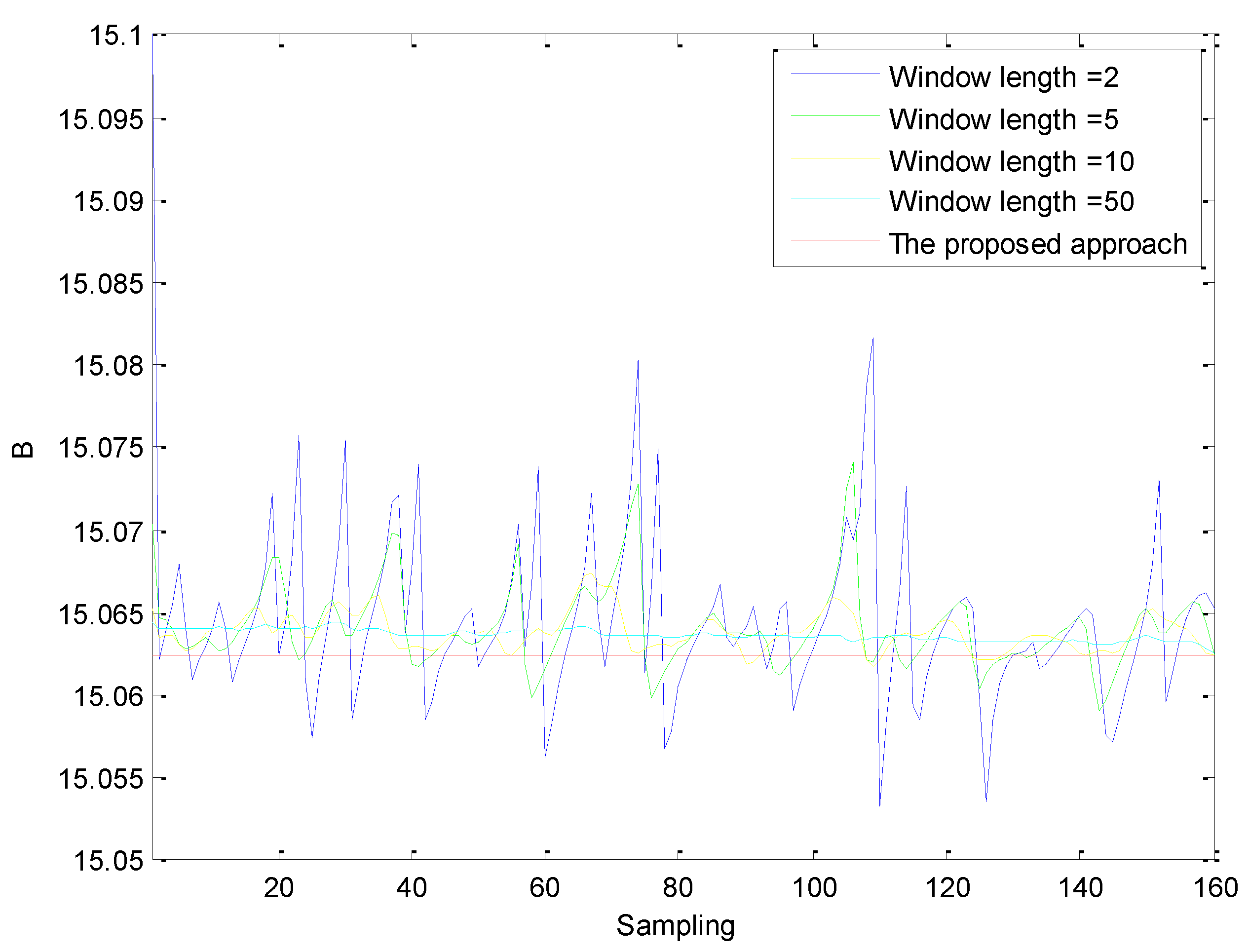
The sliding window correlation method, as a kind of conventional parameters identification method for data series, was applied to estimate the values of viscous damping coefficient by an optimization of minimizing the sums of squared errors during each observation window. Considering the sliding window is influenced with the disturbance, it is prone to change the statistical properties of the observation window. The numbers of 2, 5, 10 and 50 were chosen as the length of sliding window, and the results are seen in Figure 16.

It is seen from Figure 16 that the sliding window correlation method and the proposed approach have a similar accuracy throughout the process from sampling 1 to sampling 160. However, there are some fluctuations for the sliding window correlation method according to different window length. The shorter the length of the slide window, the more sensitive the result, and vice versa. In contrast, the proposed approach shows a fine stability owing to its episodes training.

The advantages and disadvantages of three methods are summarized in

Table 6. The comparisons of three methods.

	Advantage	Disadvantage
The BP networks	Learning algorithm, high accuracy in steady state	Worse in transient state
The sliding window correlation method	Optimization algorithm, high accuracy in steady state and transient state	Related to the length of the window and affected by disturbance
The proposed approach	high accuracy in steady state and transient state, only using the data during a period	Long training time

.

The proposed approach has the ability to obtain a high accuracy of viscous damping coefficient in steady state and transient state during only a period. To our best knowledge, there are no other approaches to implement the identification of model parameters with so little information, which is beneficial to the online control. However, it is limited to a slow process of the forging machine due to a long training time, though some improvements have been made, such as eligibility traces and heuristic search. A hardware implementation of this proposed approach is an attractive request for broader industrial processes.

5. Conclusions

In this paper, reinforcement learning has been addressed to identify optimal parameters values online by directly using raw data in one period. Compared with the BP network approach, the proposed technique has a good accuracy throughout the whole process. Compared with the sliding window correlation method, the proposed method has a similar accuracy but has a better ability to resist the influence of noise. As a result, the proposed approach has been demonstrated to be effective for online parameter identification in a simulation of real-time process of a forging machine.

References

1. Gao, Z.; Chen, M.Z.Q.; Zhang, D. Special Issue on “Advances in condition monitoring, optimization and control for complex industrial processes”. Processes 2021, 9, 664. [Google Scholar] [CrossRef]
2. Gao, Z.; Liu, X. An overview on fault diagnosis, prognosis and resilient control for wind turbine systems. Processes 2021, 9, 300. [Google Scholar] [CrossRef]
3. Gao, Z.; Dai, X.; Breikin, T.; Wang, H. Novel parameter identification by using a high-gain observer with application to a gas turbine engine. IEEE Trans. Ind. Inform. 2008, 4, 271–279. [Google Scholar] [CrossRef]
4. Available online: https://www.forging.org/producers-and-suppliers/technology/vision-of-the-future#importance (accessed on 1 May 2021).
5. Lu, X.; Huang, M. System-decomposition-based multilevel control for hydraulic press machine. IEEE Trans. Ind. Electron. 2012, 59, 1980–1987. [Google Scholar] [CrossRef]
6. Jia, C.; Wu, A.; Du, C.; Zhang, D. Variable structure control with sliding mode for a class of hydraulic nonlinear system. In Proceedings of the World Congress on Intelligent Control and Automation (WCICA), Jinan, China, 7–9 July 2010. [Google Scholar]
7. Ho, T.; Ahn, K. Speed control of a hydraulic pressure coupling drive using an adaptive fuzzy sliding-mode control. IEEE-ASME Trans. Mechatron. 2012, 17, 976–986. [Google Scholar] [CrossRef]
8. Li, C.; Wu, A.; Du, C. Speed control of hydraulic press via adaptive back-stepping. Appl. Mech. Mater. 2011, 40–41, 46–51. [Google Scholar] [CrossRef]
9. Zhang, D.; Wu, A.; Zhang, G.; Du, C. Application of the differential geometric feedback linearization to the speed control of forging machine. In Proceedings of the 2010 Chinese Control and Decision Conference, Xuzhou, China, 26–28 May 2010. [Google Scholar]
10. Lee, Y.; Kopp, R. Application of fuzzy control for a hydraulic forging machine. Fuzzy Sets Syst. 2001, 118, 99–108. [Google Scholar] [CrossRef]
11. Duan, X.; Deng, H.; Li, H. A saturation-based tuning method for fuzzy PID controller. IEEE Trans. Ind. Electron. 2013, 60, 5177–5185. [Google Scholar] [CrossRef]
12. Azari, A.; Poursina, M.; Poursina, D. Radial forging force prediction through MR, ANN, and ANFIS models. Neural Comput. Appl. 2014, 25, 849–858. [Google Scholar] [CrossRef]
13. Bharti, P.S. Process modelling of electric discharge machining by back propagation and radial basis function neural network. J. Inf. Optim. Sci. 2019, 40, 263–2778. [Google Scholar] [CrossRef]
14. Fan, B.; Lu, X.; Huang, M. A novel LS-SVM control for unknown nonlinear systems with application to complex forging process. J. Cent. South Univ. 2017, 24, 2524–2531. [Google Scholar] [CrossRef]
15. Hong, J.; Yeh, W. Application of response surface methodology to establish friction model of upset forging. Adv. Mech. Eng. 2018, 10, 1–9. [Google Scholar] [CrossRef] [Green Version]
16. Pan, Q.; Li, Y.; Huang, M. Estimation of dynamic behaviors of hydraulic forging press machine in slow-motion manufacturing process. Nonlinear Dyn. 2019, 96, 339–362. [Google Scholar] [CrossRef]
17. China Society for Technology of Plasticity CMES. Forging Manual; China Machine Press: Beijing, China, 2013. [Google Scholar]
18. Koksal, G.; Batmaz, I.; Murat, C. A review of data mining applications for quality improvement in manufacturing industry. Expert Syst. Appl. 2011, 38, 13448–13467. [Google Scholar] [CrossRef]
19. Olivier, A.; Smyth, A.W. Review of nonlinear filtering for SHM with an exploration of novel higher-order Kalman filtering algorithms for uncertainty quantification. J. Eng. Mech. 2017, 143, 04017128. [Google Scholar] [CrossRef]
20. Lu, X.; Huang, M. Novel multi-level modeling method for complex forging processes on hydraulic press machines. Int. J. Adv. Manuf. Technol. 2015, 79, 1869–1880. [Google Scholar] [CrossRef]
21. Pronzato, L.; Thierry, E. Entropy minimization for parameter estimation problems with unknown distribution of the output noise. In Proceedings of the IEEE International Conference on Acoustics, Speech, and Signal Processing, Saltlake City, UT, USA, 7–11 May 2001. [Google Scholar]
22. Slivinskas, V.; Simonyte, V. Modeling of a mechanical system using output data of the hammer blow sequence response. J. Vibroeng. 2009, 11, 120–129. [Google Scholar]
23. Ratnaweera, A.; Halgamuge, S.K.; Watson, H.C. Self-organizing hierarchical particle swarm optimizer with time-varying acceleration coefficients. IEEE Trans. Evol. Comput. 2004, 8, 240–255. [Google Scholar] [CrossRef]
24. Artyushenko, V.M.; Volovach, V.I. Nakagami distribution parameters comparatively estimated by the moment and maximum likelihood methods. Optoelectron. Instrum. Data Process. 2019, 55, 237–242. [Google Scholar] [CrossRef]
25. Ram, S.S.; Veeravalli, V.V.; Nedic, A. Distributed and Recursive parameter estimation in parametrized linear state-space models. IEEE Trans. Autom. Control 2010, 55, 488–492. [Google Scholar] [CrossRef] [Green Version]
26. Zhang, X.; Ding, F. Recursive parameter estimation and its convergence for bilinear systems. IET Control Theory Appl. 2020, 14, 677–688. [Google Scholar] [CrossRef]
27. Chen, F.; Ding, F.; Sheng, J. Maximum likelihood based recursive parameter estimation for controlled autoregressive ARMA systems using the data filtering technique. J. Frankl. Inst. 2015, 352, 5882–5896. [Google Scholar] [CrossRef]
28. Wang, Z.; Shen, Y.; Ji, Z. Filtering based recursive least squares algorithm for Hammerstein FIR-MA systems. Nonlinear Dyn. 2013, 73, 1045–1054. [Google Scholar] [CrossRef]
29. Hirokami, T.; Maeda, Y.; Tsukada, H. Parameter estimation using simultaneous perturbation stochastic approximation. Electr. Eng. Jpn. 2006, 154, 30–39. [Google Scholar] [CrossRef]
30. Ozdemir, M.C.; Eggert, T.; Straube, A. Improving the repeatability of two-rate model parameter estimations by using autoencoder networks. Prog. Brain Res. 2019, 249, 189–194. [Google Scholar] [PubMed]
31. Olaizola, J.; Bouganis, C.S.; De, A. Real-time servo press force estimation based on dual particle filter. IEEE Trans. Ind. Electron. 2020, 67, 4088–4097. [Google Scholar] [CrossRef]
32. Kaelbling, L.; Littman, M.; Moore, A. Reinforcement learning: A survey. J. Artif. Intell. Res. 1996, 4, 237–285. [Google Scholar] [CrossRef] [Green Version]
33. Sutton, R.; Barto, A. Reinforcement Learning: An Introduction; The MIT Press: Cambridge, MA, USA; London, UK, 2005. [Google Scholar]
34. Farias, V.; Moallemi, C.; Van, B.; Weissman, T. Universal Reinforcement Learning. IEEE Trans. Inf. Theory 2010, 56, 2441–2454. [Google Scholar] [CrossRef] [Green Version]
35. Watkins, J.; Dayan, P. Q-learning. Mach. Learn. 1992, 8, 279–292. [Google Scholar] [CrossRef]
36. Vamvoudakis, K.G.; Lewis, F.L. Online actor-critic algorithm to solve the continuous-time infinite horizon optimal control problem. Automatica 2010, 46, 878–888. [Google Scholar] [CrossRef]
37. Schmidhuber, J. Deep learning in neural networks: An overview. Neural Netw. 2015, 61, 85–117. [Google Scholar] [CrossRef] [PubMed] [Green Version]
38. Zhang, D.; Gao, Z.; Lin, Z. An online control approach for forging machine using reinforcement learning and taboo search. IEEE Accesses 2020, 8, 158666–158678. [Google Scholar] [CrossRef]
Figure 1. Typical structure of forging machine [38].
Processes 09 01848 g001
Figure 2. The basic frame of reinforcement learning.
Processes 09 01848 g002
Figure 3. The scheme of proposed approach.
Processes 09 01848 g003
Figure 4. A typical control process (the set speed = 0.05).
Processes 09 01848 g004
Figure 5. The episode training process of viscous damping coefficient (B was predetermined as 15).
Processes 09 01848 g005
Figure 6. The episode training process of viscous damping coefficient (B was predetermined as 20).
Processes 09 01848 g006
Figure 7. The episode training process with leakage of 0.01 ( B r = 15).
Processes 09 01848 g007
Figure 8. The episode training process with leakage of 0.01 ( B r = 20).
Processes 09 01848 g008
Figure 9. The episode training process with leakage of 0.02 ( B r = 15).
Processes 09 01848 g009
Figure 10. The episode training process with leakage of 0.02 ( B r = 20).
Processes 09 01848 g010
Figure 11. The learning process of leakage coefficient ( λ c was predetermined as 0.01).
Processes 09 01848 g011
Figure 12. The episode training process of leakage coefficient ( λ c was predetermined as 0.02).
Processes 09 01848 g012
Figure 13. The episode training process of viscous damping coefficient and leakage coefficient subject to noise of uniform distribution.
Processes 09 01848 g013
Figure 14. The episode training process of viscous damping coefficient and leakage coefficient subject to noise of Gaussian distribution.
Processes 09 01848 g014
Figure 15. The comparison between BP network and the proposed approach.
Processes 09 01848 g015
Figure 16. The comparison between the slide window and the proposed approach.
Processes 09 01848 g016