Calibration of DEM for Cohesive Particles in the SLS Powder Spreading Process

Abstract

In this paper, a new DEM calibration procedure based on two different types of procedures to compare simulation with experiments is proposed. The aim is to find the values of the interfacial adhesive surface energy and the coefficient of rolling friction between the particles to be used in the simulation. The approach adopted is the so-called Bulk Calibration method. The experimental values of the angle of repose and unconfined yield strength, found with a static testing method and by shear testing, respectively, are compared, respectively, with the angle of repose, found in a simulation reproducing the experimental procedure, and the unconfined yield strength, obtained from an idealized uniaxial testing procedure. The simulated DEM particles are spheres equipped with the Hertz Mindlin with JKR contact model. The results suggest that a bulk calibration approach is not able to provide results that are consistent with two simple bulk property evaluations and, therefore, direct ways to estimate the surface energy based on the evaluation of interparticle forces, for example, should preferably be adopted.

1. Introduction

Interest in additive manufacturing (AM) is growing in many applications, among which are biomedical, aerospace, buildings [1], due to its capability to create complex parts directly from raw materials with minimal waste and the possibility to use many types of materials such as metals, ceramics, polymers, composites [2]. Moreover, powders can be reused, making AM more affordable compared with traditional manufacturing methods [3], while other advantages are the time and cost reduction it provides [4]. Among the AM processes, Selective Laser Sintering (SLS) is a process by which artifacts are created by alternating spreading and laser sintering of layers of particles, done on the basis of a CAD file [5]. With respect to other manufacturing processes, SLS has the great advantage of being relatively inexpensive, but it has also some disadvantages, such as of being a slow process [2] and of being able to produce artifacts with size limitations, poor surface finishing [6] and low mechanical properties [2]. In particular, the latter two disadvantages are mostly related to a bad distribution of the powder in the formation step of the powder layer. Hence, the importance of focusing on the powder distribution process during the layer formation simulated both experimentally and numerically.

To understand why some irregularities of the layer are obtained, simulations using the discrete element method (DEM) can be a powerful tool [7]. DEM is a computational method by which the granular flow is simulated at the individual particle level. Often, a soft sphere approach [8] is used, in which the particles are modeled as discrete entities and their motions and trajectories are described by their translational and rotational motion, governed by the Newton’s second law [9]. To calculate the forces between the particles, as well as between the particles and the objects around the particles, DEM requires appropriate contact models. Many of these models are reported in the literature, and differ for the different features of the contact that they are able to take into account. For example, Tomas [10] discusses the models describing normal and tangential forces occurring in the contacts between two smooth spheres, including adhesive forces in presence of purely elastic deformations and elastic–plastic deformation at contact.

A model often used to describe purely elastic deformation at the particle contacts is the Hertz–Mindlin model. In this model, the normal force component between two perfectly elastic spherical objects in contact is calculated from the distance between the particle centers based on the Hertzian contact theory [11,12], while the tangential force at the contact assumes friction on the particle surface and is based on the work of Mindlin and Deresiewicz [13,14]. One of the simple methods to include adhesion forces, assuming the Hertz–Mindlin model for the elastic and friction forces, is to use the Johnson, Kendall and Roberts [15] model (JKR) in which the effect of van der Waals forces at the contact between two objects is assumed. If this model is used, a value for the interfacial adhesive surface energy between the surfaces of the interacting objects has to be assigned. Anyway, the model provides idealized contact mechanics (neglecting, for example, the effects of the surface roughness on the calculation of the adhesive force). Furthermore, it is often complicated to directly evaluate the model parameters experimentally. For this reason, the practical procedure adopted to estimate the best parameter values to be used in the model simulation is calibration.

There are two approaches reported in the literature to calibrate the DEM input parameters: the direct measuring approach and the bulk calibration approach [16]. The direct measuring approach consists of determining the property value by directly measuring it. For example, in order to simulate the powder flow during spreading in additive manufacturing, Nan et al. [7,17] used the interfacial adhesive surface energy of the JKR model, measured by the drop test method [18]. Surface energy can also be calculated from contact angle measurements using the Owens–Wendt–Rabel–Kaelble (OWRK) method or from the atomic force microscopy measurements [19]. Even if it is not always feasible, other DEM parameters can be calculated experimentally, such as: the coefficient of static friction [7,20], the coefficient of rolling friction, and the coefficient of restitution [7,21,22].

The direct measuring approach allows a deeper insight into contact physics, but requires complex experimental devices able to operate at the particle level, and is sometimes unable to consider the interdependencies between simplified approaches in the description of the model mechanics, and therefore the bulk calibration approach is often followed; this consists of the measurement of a material bulk property in experiments, which are then numerically replicated. The most appropriate DEM parameter value is found by changing its value in a replicated simulation until the experimental bulk property matches the experimental value. For example, Lupo et al. [23] used this approach to evaluate the interfacial adhesive surface energy between the particles from the comparison between the experimental and the measured interparticle cohesive force by using the Hertz–Mindlin model with the JKR model, or with the Linear cohesion model. In that case, it was demonstrated that the choice of time step in the simulation can lead to very different values of the contact force. Salehi et al. [24] used the Anton Paar powder cell to calibrate the coefficient of sliding friction, particle to particle, by comparing the experimental torque, obtained with the two-blade impellers and the DEM simulation. They also determined the coefficient of sliding friction between the particles and geometry by matching experiments and simulation predictions in the case of a circular impeller. Grima et al. [25] calibrated the coefficients of static and rolling friction as well as the coefficient of restitution by measuring the angle of repose, comparing it with the one obtained with the simulation, and by validating the DEM models through comparison of the results of the simulations against experimental slump tests and hopper discharge experiments. Alizadeh et al. [26] used the angle of repose as a way to tune the surface energy, and they observed a good agreement between the experimental and DEM simulation results. Roessler et al. [27] calibrated the sliding friction coefficient, the rolling friction coefficient, and cohesion energy density of a simplified JKR model by simulating the pull-up test of a hollow cylinder filled with bulk material. Karkala et al. [28] simulated both the dynamic yield strength test and shear cell experiment to calibrate the following DEM parameters: surface energy, coefficients of sliding and rolling friction. Coetzee [29] calibrated the contact stiffness using a confined compression test and the coefficients of sliding and rolling friction using either the individual or combined results from a draw down, rotating drum and annular ring shear test. Chen et al. [30] evaluated the sliding friction coefficient and the interfacial adhesive surface energy between the particles by comparing the macroscopic flow profile of the powder during layering between the numerical and experimental results. Angus et al. [31] combined sliding test experiments and DEM simulations of both homogeneous simple shear and the FT4 shear cell to evaluate the coefficients of rolling and sliding friction; they figured out that one single simulation type could not be sufficient to calibrate the DEM parameters. In fact, homogeneous simple shear simulations returned multiple pairs of both the coefficients. Simulations of the full FT4 shear cell with different pairs obtained with the previous simulation procedure were necessary to find the correct pair.

In order to elucidate the powder spreading process in SLS, a new experimental apparatus has been designed and built at the University of Salerno. It allows for the reproduction of different spreading conditions by changing the process conditions determined by the kind of the spreading tool and its movement parameters, such as the gap below the spreading tool, its shape, and in case of rollers the rotational velocity. Therefore, the tool is able to experimentally simulate the spreading of the powder in different configurations of the SLS apparatus, in order to understand the mechanisms that determine the formation of a layer and optimize the process conditions; however, the proper modeling of the process is necessary to gain an insight into the process.

In this work, the calibration of a DEM to be used in future for the modeling of SLS spreading is carried out. The contact model taken into consideration is the Hertz–Mindlin and JKR models to describe the contact mechanics. The use of these models is supported by the fact that the particles in the SLS spreading process do not experience high stresses and, therefore, the intrinsic limit of this model not accounting for plastic deformations at contact points may not be significant. The bulk calibration approach is used to evaluate the interfacial adhesive surface energy and the coefficient of rolling friction between the particles, while the main objective of the calibration procedure will be to find a value of the interfacial adhesive surface energy and of the coefficient of rolling friction between the particles. Two different independent calibration procedures to estimate these two parameters are proposed: one is based on the match of the static angle of repose estimated with the formation of a powder heap, as obtained on both experiments and model simulations; the other relies on the comparison between the unconfined yield strength experimentally measured with a shear testing procedure and the unconfined yield strength calculated from an idealized uniaxial testing model simulation. Each of the two calibration methods provides an independent set (couples) of values of the model interfacial adhesive surface energy and of the coefficient of rolling friction between the particles able to satisfactorily describe the experiments with the model. The scope will be to verify whether it is possible to use these two independent sets to find at least a single couple of values of the model surface energy and of the coefficient of rolling friction between the particles to be used in both model simulation procedures to satisfactorily describe all the experimental results.

2. Materials and Methods

2.1. Experimental Materials, Apparatuses and Procedures

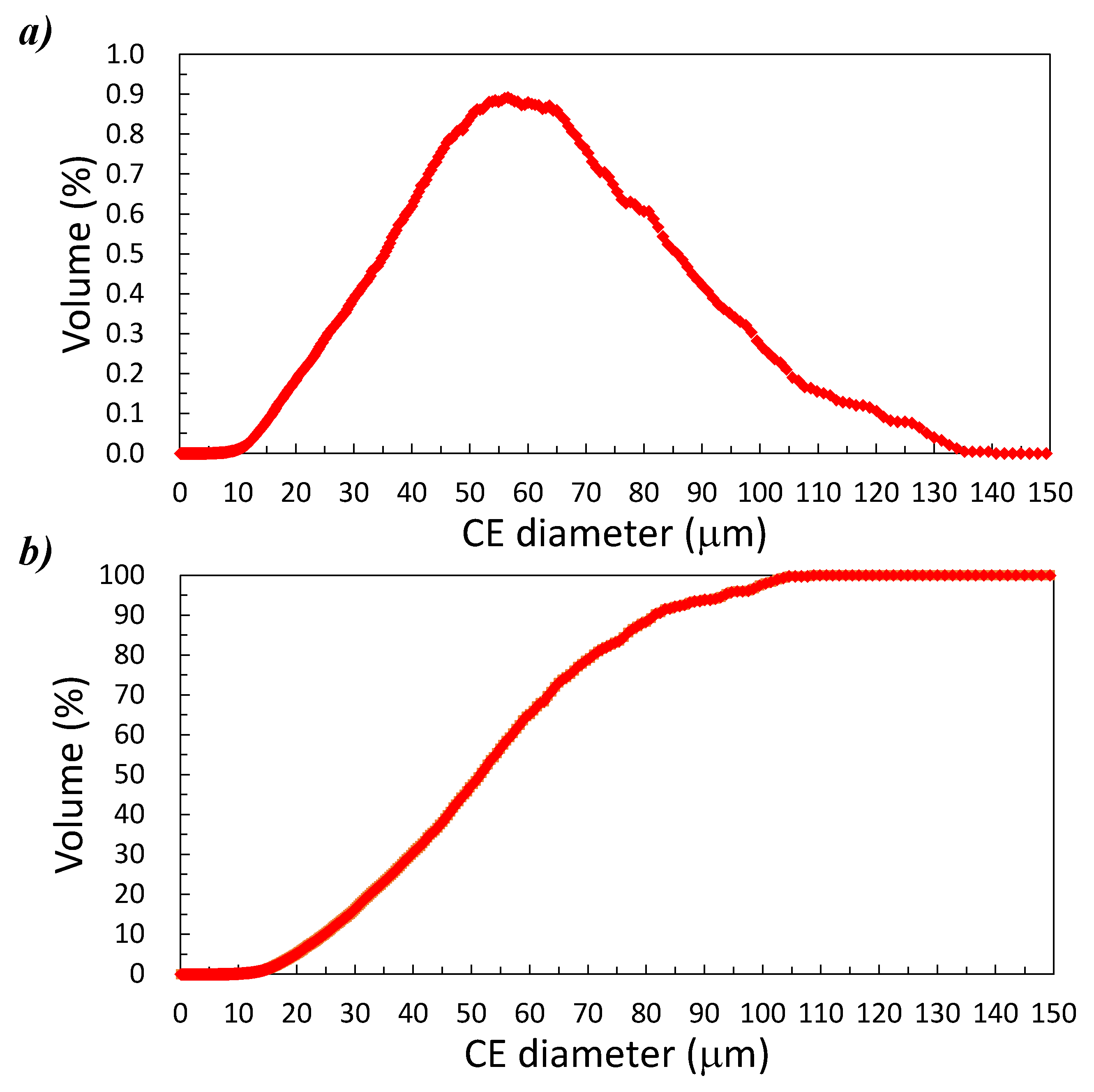
2.1.1. Materials

The polymeric powder used in the experiments to be simulated with the DEM is Domo’s Sinterline unfilled polyamide 6 3400 HT110 Natural (PA6), purposely designed for the SLS process. The material properties derived from the literature or from the technical data sheet of the powder, and used in the DEM, are reported in

Table 1. Material properties of PA6 powder to be used in the simulation: ${\mathrm{d}}_{10}$, ${\mathrm{d}}_{50}$ and ${\mathrm{d}}_{90}$ are the particle diameters corresponding to the 10th, 50th and 90th percentile of the cumulative particle size, respectively; ${\mathsf{\rho }}_{\mathrm{s}}$ is the density of the solid; ${\mathsf{\rho }}_{\mathrm{b}}$ is the bulk density of the powder. Value with reference was taken from the literature, the other values were taken from the technical data sheet of the powder.

Material	${\mathsf{d}}_{10}$ (μm)	${\mathsf{d}}_{50}$ (μm)	${\mathsf{d}}_{90}$ (μm)	${\mathsf{\rho }}_{\mathsf{s}}$ (kg m−3)	${\mathsf{\rho }}_{\mathsf{b}}$ (kg m−3)
PA6	25	55	95	1140 [32]	525

.

To characterize the shape distributions of the particles to be reproduced with the DEM, SEM images have been taken by using the TM3030Plus Tabletop Microscope (Hitachi, JP). The images are reported in Figure 1. They show that the particles are clearly non-spherical and inhomogeneous.

2.1.2. Direct Measurement of Particle Properties to Be Used in DEM

Some properties, which must be known to properly simulate the powder, were taken from the technical data sheet of the powder, such as the Young’s modulus of the particle material, or were found in the literature such as the Poisson’s ratio of the particle material and the coefficient of restitution between the particles, and these are reported in

Table 2. Properties inserted in the EDEM ™ model for the interaction between the particles (PA6) and between the particles and the geometries made of aluminium: ${\mathrm{e}}_{\mathrm{P}-\mathrm{P}}$ and ${\mathrm{e}}_{\mathrm{P}-\mathrm{G}}$ are the coefficients of restitution between the particles and between the particles and the geometry, respectively; ${\mathsf{\mu }}_{\mathrm{S}, \mathrm{P}-\mathrm{P}}$ and ${\mathsf{\mu }}_{\mathrm{S}, \mathrm{P}-\mathrm{G}}$ are the coefficient of sliding friction between the particles and between the particles and the geometry, respectively; ${\mathsf{\mu }}_{\mathrm{R}, \mathrm{P}-\mathrm{P}}$ and ${\mathsf{\mu }}_{\mathrm{R}, \mathrm{P}-\mathrm{G}}$ are the coefficient of rolling friction between the particles and between the particles and the geometry, respectively; $\mathsf{\nu }$ is the Poisson’s ratio; $\mathrm{E}$ is the Young’s modulus. Values with references were taken from the literature, while the others were taken from the technical data sheet of the powder or directly measured as described in the text. Regarding ${\mathsf{\mu }}_{\mathrm{S}, \mathrm{P}-\mathrm{G}}$ there are two rows: the first reports the values of ${\mathsf{\mu }}_{\mathrm{S}, \mathrm{P}-\mathrm{G}}$ used in the unconfined yield strength (UYS) calibration; the second reports the value of ${\mathsf{\mu }}_{\mathrm{S}, \mathrm{P}-\mathrm{G}}$ used in the static angle of repose (AOR) calibration, and which has been measured as described in the text.

Material	PA6	Aluminium
$e_{P-P}$(-)	0.5 [34]	-
$e_{P-G}$(-)	0.5 [34]
${\mu }_{S, P-P}$(-)	0.57	-
${\mu }_{S, P-G}$(-)(UYS)	1 × 10−4 ÷ 1
${\mu }_{S, P-G}$(-)(AOR)	0.33
${\mu }_{R, P-P}$(-)	1 × 10−5 ÷ 1	-
${\mu }_{R, P-G}$(-)	1 × 10−4 ÷ 1
$\nu$(-)	0.35 [35]	0.33 [36]
$E$(GPa)	3.4	69 [36]

. A procedure similar to that described by Nan et al. [1] was followed by Lupo [33] to evaluate the coefficient of sliding friction between the particles, the coefficient of sliding friction with an aluminium surface, and the heap angle. Both the coefficients of sliding friction are reported in Table 2, and the heap angle was 36.96° ± 2.5°.

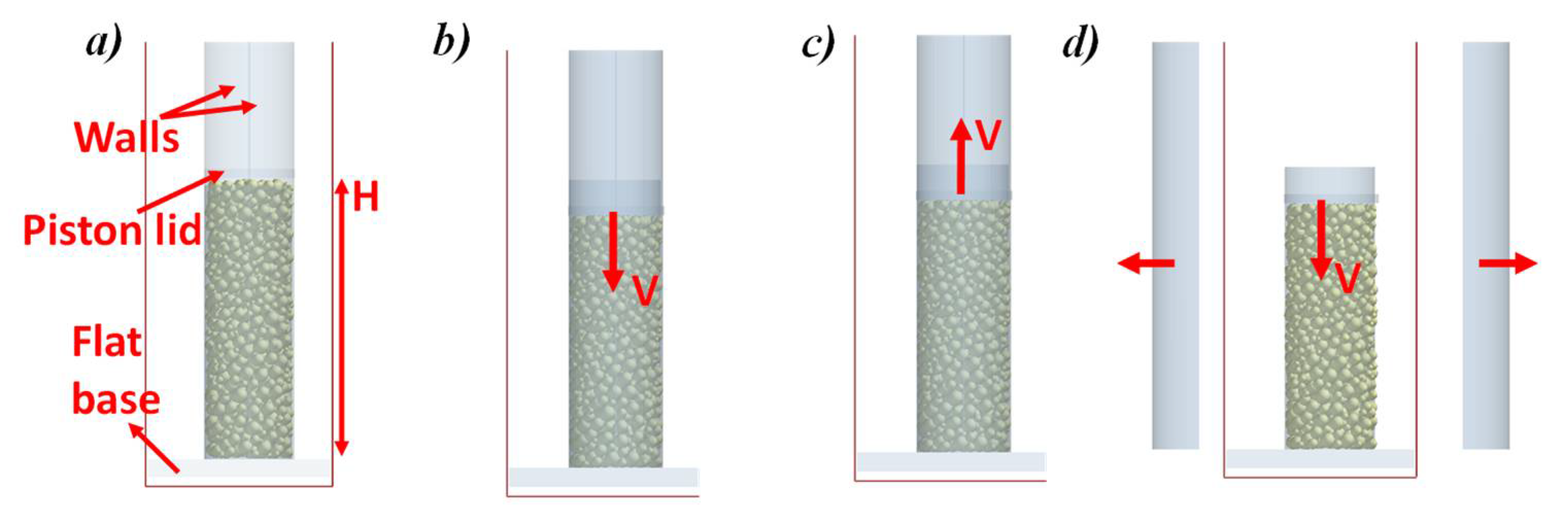
2.1.3. Experimental Setup Used for the Unconfined Yield Strength Calibration Method

A Schulze ring shear tester RST-01.01, equipped with an S-cell (internal volume of the cell of 203.58 cm³; external and internal annulus diameter of the lid of 118 and 62 mm, respectively) was used to shear test the powder and to derive the unconfined yield strength in condition of absence of consolidation, i.e., the major principal stress, ${\mathsf{\sigma }}_1$, equal to zero. Both the standard procedure recommended for the ring shear tester RST-01.01 and the ASTM-standard (ASTM D6773, 2002) were followed. Before the shear tests, the powder has been placed in the oven for 1 h at 100 °C to remove the humidity. Tests at consolidation stresses between 50 and 90 Pa were carried out and 4–5 shear points were registered to obtain the corresponding yield locus. A software application, developed in the LabVIEW environment (National Instruments), was used to acquire, visualize, and record the main data, which were measured during the shear experiments. Moreover, the RSV 95 software version 2.1.0.1 for the RST-01.01 Schulze shear tester was used to derive the unconfined yield strength of the powder from the powder yield loci.

2.2. Modelling Approach

2.2.1. DEM

DEM is a numerical procedure which allows to describe the mechanical behavior of assemblies of particles [9]. There are two main approaches that can be used to calculate contact forces: the hard-sphere approach and the soft sphere approach [8]. In the first case, each binary collision is modeled as an instantaneous process, and the properties of the particles after the collision are related to the properties of the particles before the collision by means of momentum and energy balances. Therefore, this method can be used only for those systems where multiple and simultaneous collisions are unlikely to occur, such as dilute systems. Moreover, this method cannot include long-range interparticle forces in the model [37]. On the contrary, the soft sphere approach deals with multi-particle collisions and the interparticle forces can be easily implemented, even if with higher computational time. In the soft sphere approach, the particles are modelled as individual entities and their movement is described by the translational and rotational motion, given by the Newton’s second law:

$${\mathrm{m}}_{\mathrm{i}}\frac{{\mathrm{dv}}_{\mathrm{i}}}{\mathrm{dt}}={\displaystyle \sum }_{\mathrm{j}}{\mathrm{F}}_{\mathrm{ij}}^{\mathrm{c}}+{\displaystyle \sum }_{\mathrm{k}}{\mathrm{F}}_{\mathrm{ik}}^{\mathrm{nc}}+{\mathrm{F}}_{\mathrm{i}}^{\mathrm{f}}+{\mathrm{m}}_{\mathrm{i}}\mathrm{g}$$

(1)

$$\frac{{\mathrm{d}\mathsf{\omega }}_{\mathrm{i}}}{\mathrm{dt}}=\frac{{{\displaystyle \sum }}_{\mathrm{j}}{\mathrm{F}}_{\mathrm{ij}}^{\mathrm{t}} \mathrm{R}}{{\mathrm{I}}_{\mathrm{i}}}$$

(2)

where ${\mathrm{m}}_{\mathrm{i}}$, ${\mathrm{v}}_{\mathrm{i}}$ and ${\mathsf{\omega }}_{\mathrm{i}}$ are the mass, translational velocity and angular velocity of particle $\mathrm{i}$, respectively; $\mathrm{t}$ is the time, ${\mathrm{F}}_{\mathrm{ij}}^{\mathrm{c}}$ is the contact force due to interaction between the particle $\mathrm{i}$ and the nearby ones $\mathrm{j}$ or the wall; ${\mathrm{F}}_{\mathrm{ik}}^{\mathrm{nc}}$ represents the non-contact forces like van der Waals and electrostatic forces acting on particle $\mathrm{i}$ by particle $\mathrm{k}$ or the other possible forces; ${\mathrm{F}}_{\mathrm{i}}^{\mathrm{f}}$ is the particle-fluid interaction force; ${\mathrm{F}}_{\mathrm{ij}}^{\mathrm{t}} \mathrm{R}$ is the torque imposed on particle $\mathrm{i}$ by particle $\mathrm{j}$, ${\mathrm{I}}_{\mathrm{i}}$ is the moment of inertia and $\mathrm{g}$ is the acceleration due to the gravity. By integrating (2) and (3), new velocities and positions of the particles are obtained [9,38].

To implement a DEM simulation, a contact model has to be assumed with the corresponding parameters. A contact model describes how elements behave when they come into contact with each other, i.e., describes the forces deriving from particle collisions and contacts. As a result, particle interactions are considered in the calculations. There exist a number of force models which mostly allow particles to have deformation. The deformation is modeled as an overlap between particles. Among the most used contact models are the Hertz–Mindlin (no slip) and the Hertz–Mindlin with JKR (Johnson–Kendall–Roberts) cohesive model.

The Hertz–Mindlin (no slip) is the default model used in the EDEM software (provided by DEM Solutions Ltd., Edinburgh, UK). It accounts for the effects of contact of two elastic spheres. In this model: the normal force component is based on Hertzian contact theory [11], the tangential force model is based on the work of Mindlin–Deresiewicz [13,14]. Hertz–Mindlin, along with the JKR cohesive model, is a cohesion contact model that also accounts for the influence of van der Waals forces within the contact zone and allows the user to model strongly adhesive systems, e.g., dry powders or wet materials.

According to the JKR model [15], the normal elastic contact force depends on the overlap $\mathsf{\delta }$ and the interaction parameter, i.e., the interfacial adhesive surface energy $\mathsf{\Gamma }$, as follows:

$${\mathrm{F}}_{\mathrm{JKR}}=-4\sqrt{{\mathsf{\pi }\mathsf{\Gamma }\mathrm{E}}^{*}}{ \mathrm{a}}^{\raisebox{1ex}{$3$}\!\left/ \!\raisebox{-1ex}{$2$}\right.}+\frac{4{ \mathrm{E}}^{*} }{3{ \mathrm{R}}^{*}}{ \mathrm{a}}^3$$

(3)

$$\mathsf{\delta }=\frac{{\mathrm{a}}^2}{{\mathrm{R}}^{*}}-\sqrt{\frac{4\mathsf{\pi }\mathsf{\Gamma }\mathrm{a}}{{\mathrm{E}}^{*}}}$$

(4)

where $\mathrm{a}$ is the contact radius, while ${\mathrm{E}}^{*}$ and ${\mathrm{R}}^{*}$ are the equivalent Young’s modulus and the equivalent radius, respectively, which are defined as:

$$\frac{1}{{\mathrm{E}}^{*}}=\frac{1-{\mathsf{\nu }}_{\mathrm{i}}^2}{{\mathrm{E}}_{\mathrm{i}}}+\frac{1-{\mathsf{\nu }}_{\mathrm{j}}^2}{{\mathrm{E}}_{\mathrm{j}}}$$

(5)

$$\frac{1}{{\mathrm{R}}^{*}}=\frac{1}{{\mathrm{R}}_{\mathrm{i}}}+\frac{1}{{\mathrm{R}}_{\mathrm{j}}}$$

(6)

where ${\mathrm{E}}_{\mathrm{i}}$,${ \mathsf{\nu }}_{\mathrm{i}}$, ${\mathrm{R}}_{\mathrm{i}}$, and ${\mathrm{E}}_{\mathrm{j}}$,${ \mathsf{\nu }}_{\mathrm{j}}$, ${\mathrm{R}}_{\mathrm{j}}$, are the Young’s modulus, the Poisson ratio and the radius of each sphere in contact, respectively.

The interfacial adhesive surface energy, $\mathsf{\Gamma }$, is defined as follows:

$$\mathsf{\Gamma }={\mathsf{\gamma }}_1+{\mathsf{\gamma }}_2-{\mathsf{\gamma }}_{1,2}$$

(7)

where ${\mathsf{\gamma }}_{1 }$ and ${\mathsf{\gamma }}_2$ are the surface energies of the two spheres and ${\mathsf{\gamma }}_{1,2}$ is the interface surface energy. For the special case where two spheres of the same material come into contact, the interface surface energy is zero (${\mathsf{\gamma }}_{1,2 }$= 0), thus the interfacial surface energy becomes $\mathsf{\Gamma }=2 \mathsf{\gamma }$, where ${\mathsf{\gamma }}_1={\mathsf{\gamma }}_2=\mathsf{\gamma }$. For $\mathsf{\Gamma }=0$, ${\mathrm{F}}_{\mathrm{JKR}}$ turns into a Hertz–Mindlin normal force.

The EDEM ™ software has been used to simulate both the formation of the powder pile for the measurement of the static angle of repose and the uniaxial compression test of a powder bed, with the aim of calibrating the interfacial adhesive surface energy between the particles of the Hertz–Mindlin model with the JKR model. Both the EDEM ™ 2018 and the EDEM ™ 2019 software packages, provided by DEM Solutions, Edinburgh, UK, have been used.

2.2.2. Model Tuning for SLS Applications and Calibration Procedures

By using the Hertz–Mindlin model with JKR cohesive model, elastic deformation and adhesion between the contacting particles are taken into account. Therefore, it is assumed that no plastic deformation between the particles in the contact point is involved for the powder considered. A model that does not account for the plastic deformation at contact points would be inadequate to completely describe the effects of powder consolidation. In fact, consolidation is mainly affected by two contributions: one is the increased number of contacts between the particles, the other is the increased strength of the binary forces between particles due to local plasticization of the contact point and the consequent increase of the surface of contact between particles. Several experimental results on the powder flow properties measured at increasing temperature have proven that the effect of temperature in the change of powder flow properties can only be explained by introducing the plastic deformation of the contact that is affected by temperature, which changes the particle material yield strength [39,40]. A purely elastic model, as the one considered in this paper, can only rely on the first mechanism to describe powder consolidation and, in general, may not be adequate for real powders. Nevertheless, in SLS application, powder consolidation stresses are very low and, for this special case, interparticle forces might be adequately accounted for by a purely elastic model. This also means that in the model simulation, the value of compression force is only relevant to realize the correct number of interparticle contacts. The relatively independent value of the measured unconfined yield strength of the material with the consolidation stress supports the hypothesis of purely elastic deformation of the particles at the contact points. Since the number of these contacts is directly related to bed porosity, the compression step is carried at values of the compression stress that are able to provide values of the bed porosity similar to the experimentally found in SLS processes. In order to compare simulation results with experimental results obtained with the shear tester in the powder, the experimental result obtained with this test was extrapolated to zero consolidation, which is more relevant to the SLS process. The Hertz–Mindlin model has been used also for the interaction between particles and the geometries; this means that no adhesive forces between the contacting bodies have been considered.

Spherical particles have been used to simulate the powder rather than more complicated shapes in order to reduce the simulation time. From the SEM images (Figure 1) it appears evident that the polymeric powder is constituted by particles with different and irregular shapes. Initially, in order to replicate the actual shape of the particles, it has been tried to model them as clumped spheres [41,42] that is each particle can be approximated by a number of overlapping spheres of different sizes. However, by using this approach, simulations were excessively long, even if the particles were modelled as two or three clumped spheres. This is due to two different reasons: the first is the increase of the particles involved to simulate the powder; the second reason is that particles, which were already small, were modeled with particles even smaller and, consequently, the simulation time greatly increased. In fact, the simulation time step is chosen as a fraction of the Rayleigh time step, i.e., the natural oscillation period of the mass-spring system made by the particle and the elastic contact [43]. The Rayleigh time ($\Delta {\mathrm{t}}_{\mathrm{R}}$) depends on the particle diameter according to the following relationship:

$$\Delta {\mathrm{t}}_{\mathrm{R}}=\frac{\mathsf{\pi } \mathrm{R} \sqrt{{\mathsf{\rho }}_{\mathrm{p}}/\mathrm{G}}}{0.1631 \mathsf{\nu } +0.8766}$$

(8)

where $\mathrm{R}$ is the particle radius, ${\mathsf{\rho }}_{\mathrm{p}}$ is the particle density, $\mathrm{G}$ is the shear modulus and $\mathsf{\nu }$ is the Poisson’s ratio of the particle.

Therefore, the smaller the spheres used to model the particles, the slower the simulation.

The particle size distribution of the powder has been approximated to a purely Gaussian distribution, centered in ${\mathrm{d}}_{50}$ = 55 μm, with a width 3 $\mathsf{\sigma }$, such that:

$$3 \mathsf{\sigma }={\mathrm{d}}_{50}-{\mathrm{d}}_{10}$$

(9)

By doing so, particles smaller than ${\mathrm{d}}_{10}$ and bigger than ${\mathrm{d}}_{90}$ have been cut out. Indeed, if particles smaller than ${\mathrm{d}}_{10}$ were considered, the time step would have been too small and the simulation time would have been too long. This approximation seems to be reasonable, as demonstrated (Figure 2) by the shape of the frequency particle size distribution (PSD) and of the cumulative one, based on the equivalent circle particle diameter (CE), as obtained with the Morphologi G3 (Malvern Panalytical Ltd., Malvern, UK). CE is the diameter of a circle with the same area as the 2D image of the particle.

2.2.3. DEM Calibration Methods

DEM Calibration Using the Static Angle of Repose

Simulation of the static angle of repose resembles the experimental procedure. Inside the hopper, a dynamic virtual factory creates particles in a random way (Figure 3). The particles fall through the hole of the hopper and then they deposit on a layer of particles of the same powder; indeed, this layer is created immediately before the fall of the particles. By doing so, the experimental situation of the angle of repose test where fresh powder deposits on a previously deposited powder is replicated, while when a clearly visible heap is obtained, the creation of the particles is interrupted within the factory. The angle of repose is measured once the particles are all steady, while the hopper is a truncated cone. The radii of the bases are 100 and 400 μm, while the height of the cone is 1 mm. The properties of the powder and of the geometries, which have been used, are those reported in Table 1 and Table 2.

In the case of the simulation of the angle of repose, 40 CPUs have been used and the simulation time is approximately 8 h.

DEM Calibration Using the Unconfined Yield Strength

There are two methods to measure the unconfined yield strength of a cohesive powder subject to compression [44]. The simplest is to use a uniaxial tester in which the powder is inserted in a cylindrical mold. The powder is compressed with a piston lid to a defined consolidation stress, then when the compression force is released, the mold is open in order to free the agglomerated powder sample. If the compression force is sufficiently high, the compressed powder sample is agglomerated and is able to keep the shape of the cylindrical mold. The piston lid is then lowered again and the force necessary to break the cylindrical agglomerate is measured. The ratio between this force and the agglomerate cross section is the unconfined yield strength of the material, which is a function of the normal stress in the compression step. Unfortunately, in this procedure, it is very difficult to avoid the effect of the wall shear stress on the sample, reducing the effective compression force at the bottom of the sample [45] unless complex devices are used. For this reason, a second method is more often followed, and the unconfined yield strength is indirectly measured from shear testing experiments [46]. It is assumed that the major principal stress obtained from the Mohr circle describing the stress state during shear testing consolidation coincides with the consolidation stress in the uniaxial test and that the yield condition in the uniaxial tester is represented by the Mohr circle passing through the origin of the $\mathsf{\tau }-\mathsf{\sigma }$ plane and tangent to the static yield locus obtained with the shear tester at the same consolidation condition. This latter procedure was used to calculate the flow function of the material, i.e., the unconfined yield strength as a function of the major principal stress at consolidation. Simulation of the shear testing procedure is quite cumbersome with the DEM procedure, due to the length of the test, the number of particles to be used and complexity of the shear tester geometry. Conversely, by using a virtual experiment in DEM it is possible to easily eliminate wall friction, and therefore, an idealized uniaxial testing procedure was used to calibrate unknown DEM parameters and compare the obtained unconfined yield strength, f_c(sim), with the value indirectly measured in shear testing experiments, f_c(exp), (Figure 4).

The geometry is the one represented in Figure 5a. The mold is made by a flat base and two hemicylindrical walls that are kept fixed on the base during the compression step and removed during the yield step. In order to eliminate wall shear stress, the coefficient of sliding friction and the coefficient of rolling friction between the particles and the wall are put to a very low value (10⁻⁴) in the compression step. This idealized approach makes the size of the sample less significant. Thus, in order to minimize the number of particles used in the experiment, the diameter of the mold was set to 0.5 mm and the mold height to around 1.5 mm, that is three times the mold diameter. The simulation consists of four steps (Figure 5): (a) generation of the powder bed inside the mold; (b) compaction of the bed with a circular piston lid to achieve the desired consolidation stress in correspondence of a powder bed porosity of about 0.55; (c) raising of the lid to zero out the force exerted by the lid on the powder bed; (d) unconfined compression of the powder bed by means of the lid.

The powder bed has been created by a static factory within the mold (Figure 5a). This factory allows to create particles with a random arrangement instantly. The total mass of the powder bed used is 1.4 × 10⁻⁷ kg. Properties of the powder or regarding the interaction between the particles and the geometries, which have been used in the simulation, are reported in Table 1 and Table 2.

In order to avoid the effect of powder weight on the stress acting at the bottom of the sample, simulations have been carried out by setting the acceleration due to the gravity equal to 0 m/s².

The general rule for the implementation of the model is that the time step should be between 10 and 40% of critical Rayleigh time step [43], as suggested in the EDEM ™ 2019.2 documentation. In this work, time steps of 20 and 40% of the critical time step have been used to verify the reliability of the measured unconfined yield strength. Once the bed is created in the cylindrical factory, a piston lid (Figure 5b) with the same diameter of the powder bed compacts the bed going down at a scrolling velocity, V, of 0.005 ms⁻¹. To guarantee roughly the same initial void fraction of the polymeric powder in all the simulations and to evaluate the unconfined yield strength in correspondence of a major principal stress close to 0 Pa, the lid is stopped when the consolidation stress obtained during the compaction is almost the lowest major principal stress that the powder has experienced during the shear tests, i.e., 988 Pa. At this point, the lid is moved up to its initial position at the same velocity as the compaction step (Figure 5c). During this stage, the bed relaxes because of the elastic behavior of the particles. Then, the lid is moved down again at V = 0.001 ms⁻¹ (Figure 5d) and the hemicylindrical walls of the cylinder are removed sideways in opposite directions at V = 0.05 ms⁻¹. The absence of adhesive forces between the particle and the wall ensures that this movement of the mold does not produce any traction stress on the powder that would affect its state of consolidation. During this step, the coefficient of rolling friction and of sliding friction between the particles and the lid and between the particles and the base is increased from 1 × 10⁻⁴ to 1 to avoid particles from sliding on the wall of the geometries during the compression step. In fact, in previous simulations, where both the coefficients were maintained at low values, i.e., 1 × 10⁻⁴, the whole powder bed slipped away during the compression, preventing its deformation.

For the simulation, four CPUs have been used and the simulation time has been about 2 days.

The unconfined compression stage is carried out by imposing a downward movement to the lid and by registering, step by step, the total force exerted by the lid on the powder bed. In a real uniaxial experiment, the maximum of this force divided by the cross section of the bed should correspond to the unconfined yield strength. In fact, it corresponds with the fracture of the bed and the loss of its strength. However, in the numerical calculations, the force measured on the lid follows the general trend reported in Figure 6. The figure reports the force relative to the whole simulation in two panes. Figure 6a reports the force as a function of time, while Figure 6b reports the force as a function of the lid position. The first peak (point A) corresponds to the initial compaction of the bed before the unconsolidated compression. It appears that during the unconfined compression, the force does not reach a maximum value, but the lid continues to move for a long lid displacement without significant change; in fact, the force reaches a plateau value. The kinds of bed deformation observed are reported in Figure 7, and it appears clearly that in the simulations, the bed starts shearing without breaking (Figure 7b). Only after long time and at very large bed deformations does the force start increasing again and raises above the plateau value, due to the limited space remaining available for the bed compression. In the simulation, particles cannot fall due to the lack of gravity, but particles might, in principle, detach. This happens only at very low values of $\mathsf{\Gamma }$ (Figure 7a). In order to compare simulation results with the experiment, the yield of the powder is assumed to happen at the attainment of the plateau value of the compression force, that has been used to calculate the unconfined yield strength. In particular, an average value of the force among those obtained before the sudden increase has been used as the plateau value.

Measured values of the unconfined yield strength (${\mathrm{f}}_{\mathrm{c}}$) as function of the coefficient of rolling friction (${\mathsf{\mu }}_{\mathrm{R}, \mathrm{P}-\mathrm{P}}$) provided a fixed value of $\mathsf{\Gamma }$ have been reported in a plot. Fitting these values of ${\mathrm{f}}_{\mathrm{c}}$ with a regression line, the couple of the parameters (${\mathsf{\mu }}_{\mathrm{R}, \mathrm{P}-\mathrm{P}}$, Γ) which gives the experimental ${\mathrm{f}}_{\mathrm{c}}$ is the desired one.

3. Results and Discussion

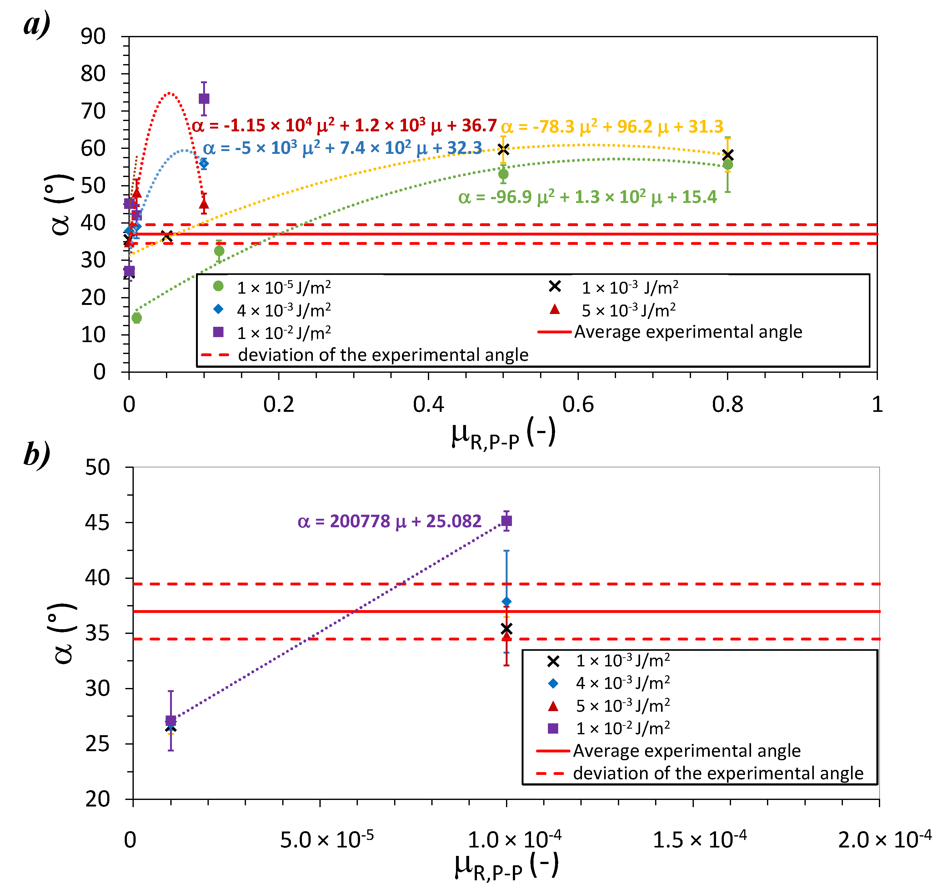
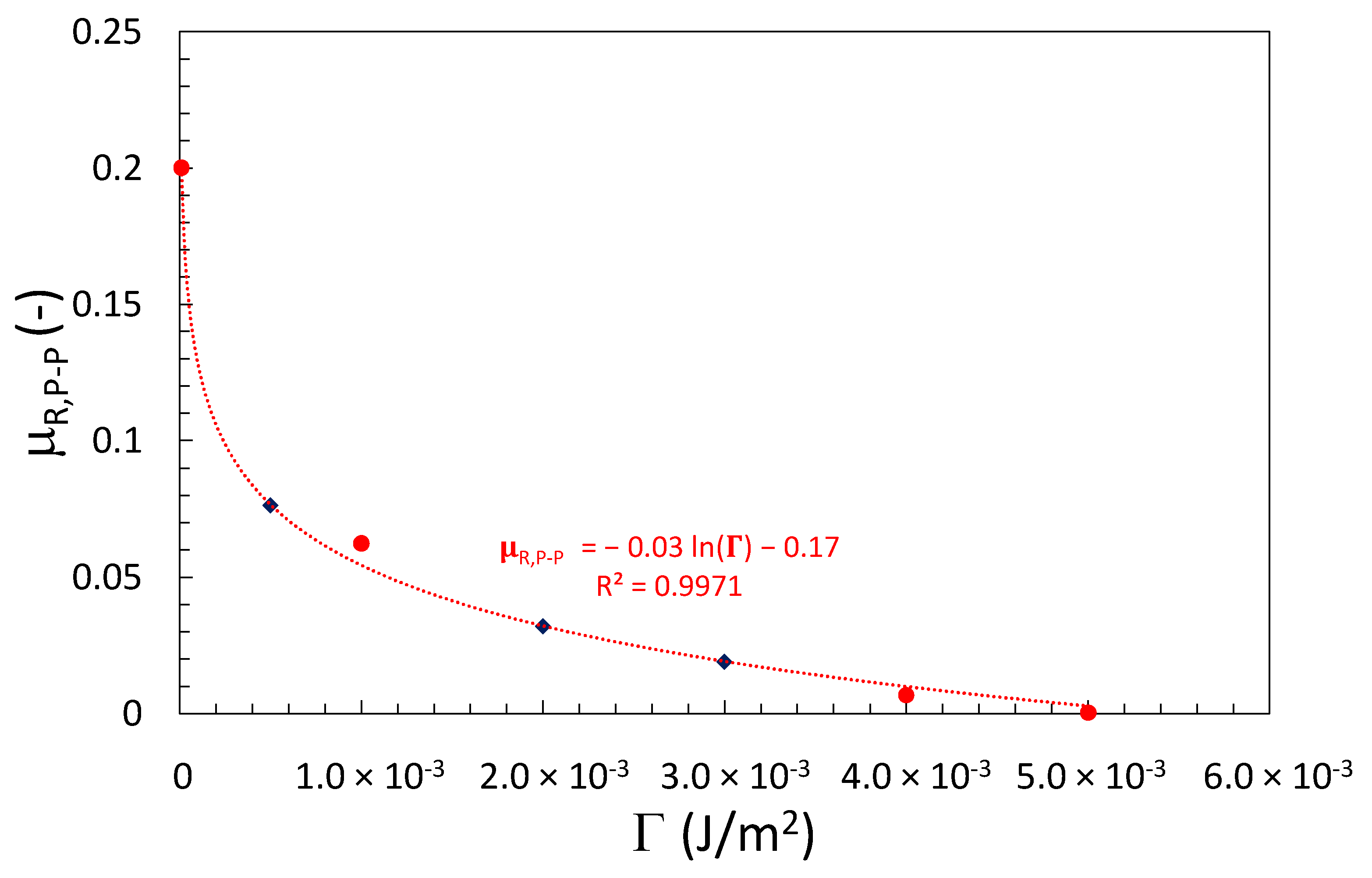
3.1. Calibration According to the Static Angle of Repose

The static angle of repose has been measured with the setup and by following the procedure described in Section 2.1.3 using six repetitions was 36.96° ± 2.5°, where the deviation reported is the standard deviation of results. Different simulations have been carried out to reproduce the formation of the heap and to evaluate the corresponding static angle of repose by choosing a time step of 40% of critical Rayleigh time step. Indeed, this time step guarantees the same value of the angle, which can be obtained with a lower percentage value, e.g., 20%. Five different values of $\mathsf{\Gamma }$ have been chosen in the range between 10⁻⁵ and 10⁻² J/m². For each value of $\mathsf{\Gamma }$, different values of the coefficient of rolling friction between the particles (${\mathsf{\mu }}_{\mathrm{R}, \mathrm{P}-\mathrm{P}}$) have been used ranging between 10⁻⁵ and 0.8. The aim is to find the pairs of the parameters for which the experimental static angle of repose, $\mathsf{\alpha }$(exp), is matched by the one obtained by the simulations, $\mathsf{\alpha }\left(\mathrm{sim}\right)$, (Figure 8).

Results are reported in Figure 9, where the value of angle of repose resulting from simulation ($\mathsf{\alpha }$) is plotted as a function of the interfacial adhesive surface energy and the coefficient of rolling friction between the particles. Since the value of $\mathsf{\alpha }$ is estimated with a visual procedure, the simulation result is subject to a certain variation represented by error bars. Points corresponding to the same $\mathsf{\Gamma }$ are plotted using the same symbol. In the figure, the experimental value of the angle of repose is reported as a continuous red horizontal line. The two parallel red hyphenated lines represent the standard deviation of the measured value obtained by experiment repetition. Figure 9a also reports interpolating polynomial for each set of data at similar $\mathsf{\Gamma }$. Intersections of these polynomials with the horizontal line representing the experimental $\mathsf{\alpha }$ help to find couples (${\mathsf{\mu }}_{\mathrm{R}, \mathrm{P}-\mathrm{P}}$, $\mathsf{\Gamma }$) that are able to predict the correct value of the angle of repose. To verify the reliability of the results, new simulations have been carried out by setting the parameters for the four couples (${\mathsf{\mu }}_{\mathrm{R}, \mathrm{P}-\mathrm{P}}$, $\mathsf{\Gamma }$) found with the procedure above. Resulting values of α are reported in

Table 3. Comparison between the predicted $\mathsf{\alpha }$ ($\mathsf{\alpha }$ from the polynomial) and the one obtained from the simulations (${\mathsf{\alpha }}_{\mathrm{sim}}$ ) for the reported pairs of the parameters (Γ and ${\mathsf{\mu }}_{\mathrm{R},\mathrm{P}-\mathrm{P}}$ ) to verify the reliability of the prediction. $\mathsf{\sigma }$ is the standard deviation of ${\mathsf{\alpha }}_{\mathrm{sim}}$.

Γ (J/m2)	μR, P−P (-)	$\mathsf{\alpha }$ from the Polynomial (°)	${\mathsf{\alpha }}_{\mathbf{sim}}$ (°)	$\mathsf{\sigma }$ (°)
1 × 10−5	2 × 10−1	36.96	39.36	5.90
1 × 10−3	6.2 × 10−2	36.96	36.09	2.16
4 × 10−3	6.7 × 10−3	36.96	35.75	0.30
5 × 10−3	2.2 × 10−4	36.96	41.02	0.10

, which shows that the procedure is fairly adequate.

Figure 10 reports the couple of the parameters (${\mathsf{\mu }}_{\mathrm{R}, \mathrm{P}-\mathrm{P}}$, $\mathsf{\Gamma }$) represented as red circles on a plane. The best interpolating function for points in this plot is a logarithmic function:

$${\mathsf{\mu }}_{\mathrm{R}, \mathrm{P}-\mathrm{P}}=-0.032\times \ln \mathsf{\Gamma }-0.167$$

(10)

To verify the reliability of the equation, three other pairs of the parameters from the curve in the same range of $\mathsf{\Gamma }$ and ${\mathsf{\mu }}_{\mathrm{R}, \mathrm{P}-\mathrm{P}}$_, reported as blue rhumbs in Figure 10, have been chosen. By using these pairs, the value obtained of $\mathsf{\alpha }$ from the simulation is very close to the experimental one (

Table 4. Pairs of parameters ($\mathsf{\Gamma }$ and ${\mathsf{\mu }}_{\mathrm{R},\mathrm{P}-\mathrm{P}}$ ) from the logarithmic curve for which the experimental $\mathsf{\alpha }$ and that obtained from the simulation (${\mathsf{\alpha }}_{\mathrm{sim}}$ ) are matched. $\mathsf{\sigma }$ is the standard deviation of $\mathsf{\alpha }$ from the simulation.

$\mathsf{\Gamma }$ (J/m2)	${\mathsf{\mu }}_{\mathsf{R},P-P}$ (-)	$\mathbf{Experimental} \mathsf{\alpha }$ (°)	${\mathsf{\alpha }}_{\mathbf{sim}}$ (°)	$\mathsf{\sigma }$ (°)
2 × 10−3	3.2 × 10−2	36.96	38.63	0.05
3 × 10−3	1.9 × 10−2	36.96	39.18	2.33
5 × 10−4	7.6 × 10−2	36.96	39.39	0.78

). This proves that all the pairs of the logarithmic curve are all possible candidates.

In the case of $\mathsf{\Gamma }$= 1 × 10⁻² J/m², represented in Figure 9b, a regression line between the points representing $\mathsf{\alpha }$ at ${\mathsf{\mu }}_{\mathrm{R}, \mathrm{P}-\mathrm{P}}$ = 10⁻⁴ and at ${\mathsf{\mu }}_{\mathrm{R}, \mathrm{P}-\mathrm{P}}$ = 10⁻⁵ has been considered to have a best estimation of the coefficient of rolling friction in case of ${\mathsf{\Gamma }}_{\mathrm{P}-\mathrm{P}}$ = 1 × 10⁻² J/m². From the line, a value of ${\mathsf{\mu }}_{\mathrm{R}, \mathrm{P}-\mathrm{P}}$ = 5.92 × 0⁻⁵ has been obtained. Repeating the simulation with this value of ${\mathsf{\mu }}_{\mathrm{R}, \mathrm{P}-\mathrm{P}}$, the resulting static angle of repose is 42.6 ± 1.6, which is somewhat higher than the experimental angle, compared to the other values of $\mathsf{\alpha }$ obtained from the simulations with the other pairs of parameters of Table 3 and Table 4. Therefore, it is better to consider values of $\mathsf{\Gamma }$ between 1 × 10⁻⁵ and 5 × 10⁻³ J/m² as possible candidates.

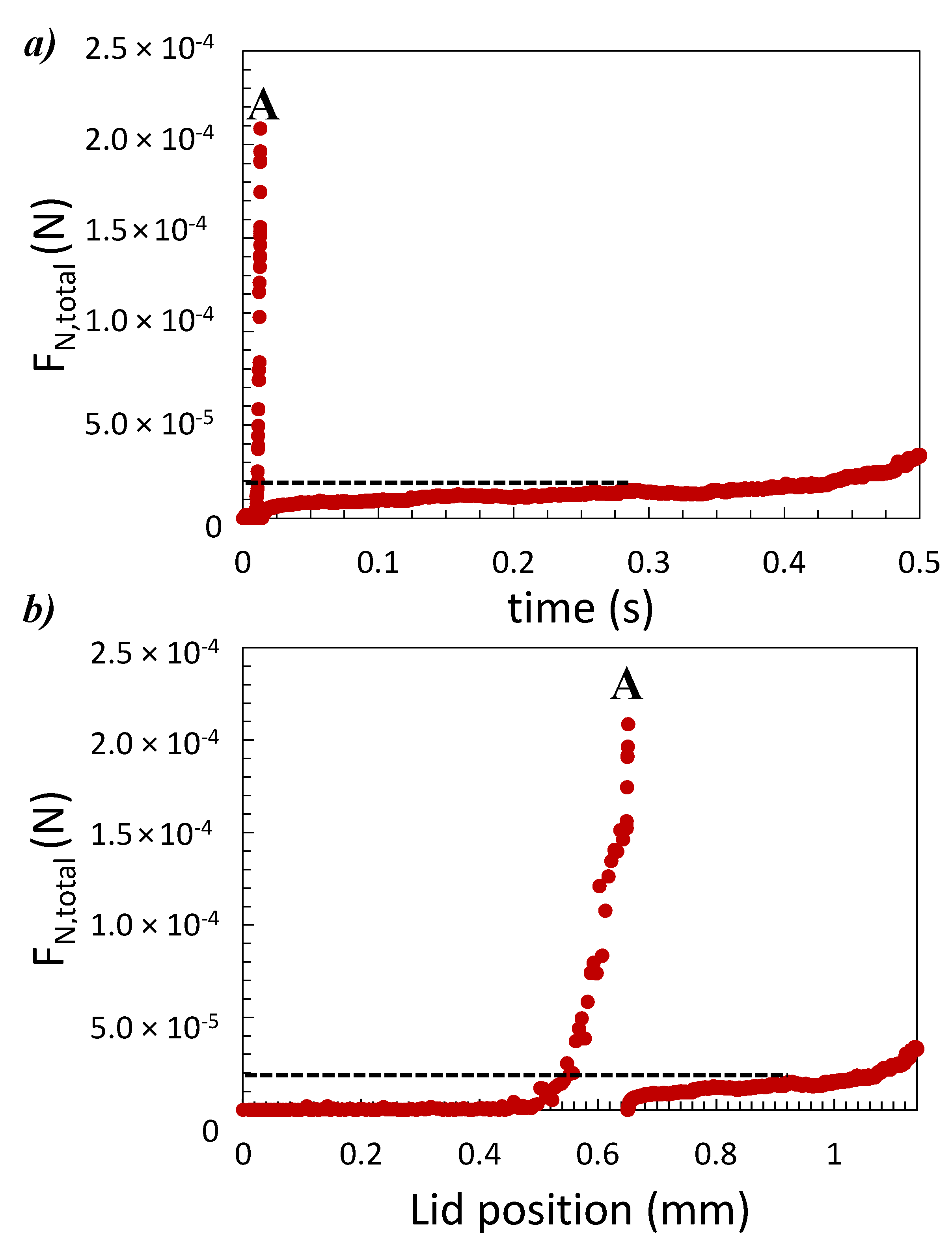
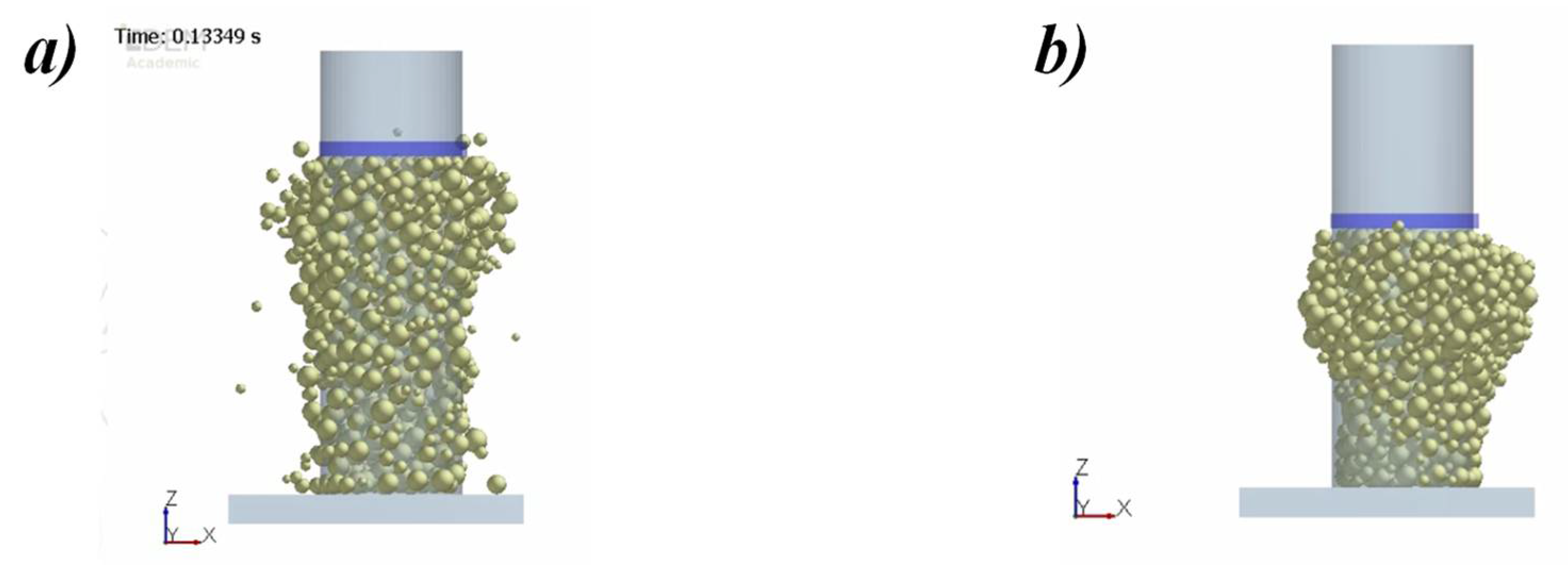
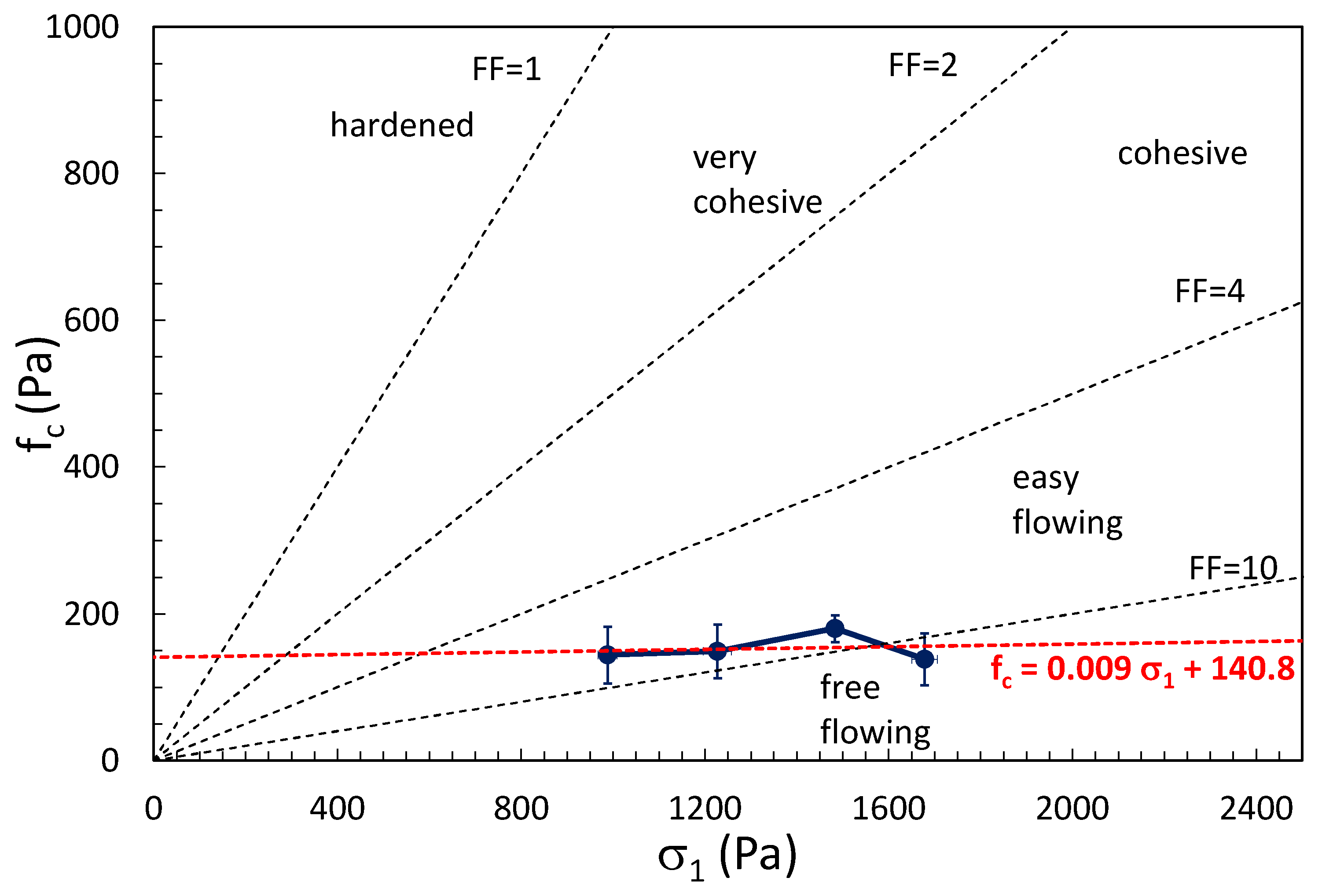
3.2. Calibration According to the Unconfined Yield Strength

Four different tests at different maximum loads (0.4, 0.5, 0.6, and 0.7 kg) have been carried out with the shear tester. To verify the reproducibility of the measurements, each test has been repeated three times. A value of ${\mathrm{f}}_{\mathrm{c}}$ has been measured for each value of ${\mathsf{\sigma }}_1$. The average values of ${\mathrm{f}}_{\mathrm{c}}$, obtained from the repetition, have been reported in Figure 11, where the flow factors (FF = ${\mathsf{\sigma }}_1$/${\mathrm{f}}_{\mathrm{c}}$), which limit the Jenike flowability classes [47], are reported as hyphenated lines. Data show that at ambient temperature and for ${\mathsf{\sigma }}_1$> 1600 Pa the powder is free flowing (FF > 10), while for 975 < ${\mathsf{\sigma }}_1$< 1600 Pa, the polyamide 6 is easy flowing (4 < FF < 10). The good flowability of this polyamide is not surprising, being that the powder specifically engineered for the SLS process. Significantly, the variation of the unconfined yield strength is not very much affected by the compression stress. The unconfined yield strength has been extrapolated at ${\mathsf{\sigma }}_1$ = 0 Pa from the regression line (red hyphenated line in Figure 11). Its value is about 141 Pa.

With the aim of finding new pairs, values of $\mathsf{\Gamma }$ and of the coefficient of rolling friction have been sought comparing the experimental values of the unconfined yield strength and the model results of uniaxial idealized test. Time steps of 20 and 40% of Rayleigh time step were adopted. In these simulations, $\mathsf{\Gamma }$ has been set between 10⁻⁵ and 10⁻² J/m² and ${\mathsf{\mu }}_{\mathrm{R}, \mathrm{P}-\mathrm{P}}$ has been changed between 0.1 and 1. Results are reported in Figure 12. The error bars correspond to different values obtained by measuring ${\mathrm{f}}_{\mathrm{c}}$ with a time step of 20% and 40%. The bars are quite short and it proves that the measured value does not change much if the time step is varied in the aforementioned range. In the tested range, it was possible to find only a single couple (${\mathsf{\mu }}_{\mathrm{R}, \mathrm{P}-\mathrm{P}}$, $\mathsf{\Gamma }$) for which the experimental ${\mathrm{f}}_{\mathrm{c}}$ is matched by ${\mathrm{f}}_{\mathrm{c}}$ from the simulation, and it is provided by the intersection of the regression line of simulation results corresponding to $\mathsf{\Gamma }$ = 1 × 10⁻² J/m², with the red line corresponding to the experimental value of ${\mathrm{f}}_{\mathrm{c}}$. The intersection occurs at ${\mathsf{\mu }}_{\mathrm{R}, \mathrm{P}-\mathrm{P}}$ = 0.326 and, correspondingly, the ${\mathrm{f}}_{\mathrm{c}}$ obtained from the simulations is 141 ± 7 Pa.

In the case of 10⁻⁵ J/m², for ${\mathsf{\mu }}_{\mathrm{R}, \mathrm{P}-\mathrm{P}}$ < 0.8 it was not possible to find any simulation value for ${\mathrm{f}}_{\mathrm{c}}$ because the particles separated before the unconfined compression due to the very low values of resulting forces keeping them together. This case is the one reported in Figure 7a. From Figure 12 it appears that the higher the $\mathsf{\Gamma }$, the higher is the resulting ${\mathrm{f}}_{\mathrm{c}}$, fixed the value of ${\mathsf{\mu }}_{\mathrm{R}, \mathrm{P}-\mathrm{P}}$. In fact, the higher the value of $\mathsf{\Gamma }$, the higher the van der Waals attractive force between the particles and, correspondingly, the higher ${\mathrm{f}}_{\mathrm{c}}$ becomes.

The comparison between Figure 9 and Figure 12 shows that the only value of the interfacial adhesive surface energy for which both the experimental α and ${\mathrm{f}}_{\mathrm{c}}$ are matched by the ones from the simulations is $\mathsf{\Gamma }$ = 1 × 10⁻² J/m². However, this happens with different coefficients of the rolling friction namely with a value of ${\mathsf{\mu }}_{\mathrm{R}, \mathrm{P}-\mathrm{P}}$ close to 5 × 10⁻⁵, calibrating results using the angle of repose simulation, and with a value of ${\mathsf{\mu }}_{\mathrm{R}, \mathrm{P}-\mathrm{P}}$ = 0.326, in the case of the unconfined compression test simulation. Therefore, it would seem that using DEM as we have done, adopting the Hertz–Mindlin contact model with the JKR model for cohesion, it is not possible to calibrate the model so that it can contemporarily reproduce the correct values of the unconfined yield strength and of the static angle of repose. This disappointing result may be related with the other circumstance that we have observed above, regarding the lack of an apparent yield with a maximum of the compression force in the uniaxial unconfined compression test, suggesting that the model used is not able to properly describe the powder shear mechanisms during the unconfined yield. It may be that alternative contact models, or the use of different particle shapes, should be tried to verify if the DEM model is able to describe with the same calibration parameters the unconfined yield and the correct static angle of repose.

A different method was used by Lupo [33], based on the approach developed by Ruggi et al., by extrapolating the tensile strength of the powder from a linearized yield locus and by calculating from this the theoretical pull off force the Rumpf equation. This approach provides a value for the surface energy of $\mathsf{\Gamma }$ = 2 × 10⁻³ J/m², for which a value of ${\mathsf{\mu }}_{\mathrm{R}, \mathrm{P}-\mathrm{P}}$ = 1.9 × 10⁻¹ should be applied.

4. Conclusions

In this paper, a calibration procedure, based on the comparison between the results obtained from two different comparisons between simulation and experimental results, has been proposed to determine the interfacial adhesive surface energy between the particles of the Hertz–Mindlin model with the JKR model as well as the coefficient of rolling friction between the particles. These comparisons involve the evaluation of the static angle of repose from the formation of the powder heap and of the unconfined yield strength from the uniaxial compression test. The results of the simulations show that the two calibration procedures are not able to provide a single set of calibrated parameters. More direct ways to estimate the surface energy based on the evaluation of interparticle forces are suggested, rather than using a bulk calibration approach.

References

1. Ngo, T.D.; Kashani, A.; Imbalzano, G.; Nguyen, K.T.Q.; Hui, D. Additive Manufacturing (3D Printing): A Review of Materials, Methods, Applications and Challenges. Compos. Part B Eng. 2018, 143, 172–196. [Google Scholar] [CrossRef]
2. Tofail, S.A.M.; Koumoulos, E.P.; Bandyopadhyay, A.; Bose, S.; O’Donoghue, L.; Charitidis, C. Additive Manufacturing: Scientific and Technological Challenges, Market Uptake and Opportunities. Mater. Today 2017, 21, 22–37. [Google Scholar] [CrossRef]
3. Liu, S.; Shin, Y.C. Additive Manufacturing of Ti6Al4V Alloy: A Review. Mater. Des. 2019, 164, 107552. [Google Scholar] [CrossRef]
4. Wong, K.V.; Hernandez, A. A Review of Additive Manufacturing. ISRN Mech. Eng. 2012, 2012. [Google Scholar] [CrossRef] [Green Version]
5. Sofia, D.; Lupo, M.; Barletta, D.; Poletto, M. Validation of an Experimental Procedure to Quantify The Effects of Powder Spreadability on Selective Laser Sintering Process. Chem. Eng. Trans. 2019, 74, 397–402. [Google Scholar] [CrossRef]
6. Kumbhar, N.N.; Mulay, A.V. Post Processing Methods Used to Improve Surface Finish of Products Which Are Manufactured by Additive Manufacturing Technologies: A Review. J. Inst. Eng. Ser. C 2018. [Google Scholar] [CrossRef]
7. Nan, W.; Pasha, M.; Bonakdar, T.; Lopez, A.; Zafar, U.; Nadimi, S.; Ghadiri, M. Jamming during Particle Spreading in Additive Manufacturing. Powder Technol. 2018, 99, 481–487. [Google Scholar] [CrossRef]
8. Di Renzo, A.; Di Maio, F.P. Comparison of Contact-Force Models for the Simulation of Collisions in DEM-Based Granular Flow Codes. Chem. Eng. Sci. 2004, 59, 525–541. [Google Scholar] [CrossRef]
9. Cundall, P.A.; Strack, O.D.L. A Discrete Numerical Model for Granular Assemblies. Géotechnique 1979, 29, 47–65. [Google Scholar] [CrossRef]
10. Tomas, J. Mechanics of Nanoparticle Adhesion—A Continuum Approach. Part. Surf. Detect. Adhes. Removal. 2003, 8, 1–47. [Google Scholar]
11. Hertz, H. Über Die Berührung Fester Elastischer Körper. J. Die Reine Und Angew. Math. 1881, 92, 156–171. [Google Scholar]
12. Dintwa, E.; Tijskens, E.; Ramon, H. On the Accuracy of the Hertz Model to Describe the Normal Contact of Soft Elastic Spheres. Granul. Matter 2008, 10, 209–221. [Google Scholar] [CrossRef]
13. Mindlin, R.D.; Deresiewicz, H. Elastic Spheres in Contact Under Varying Oblique Forces. In The Collected Papers of Raymond D. Mindlin Volume I; Springer: New York, NY, USA, 1989; Volume 20, pp. 269–286. [Google Scholar] [CrossRef]
14. Mindlin, R.D. Compliance of Elastic Bodies in Contact. J. Appl. Mech. 1989, 16, 197–206. [Google Scholar] [CrossRef]
15. Johnson, K.L.L.; Kendall, K.; Roberts, A.D.D. Surface Energy and the Contact of Elastic Solids. Proc. R. Soc. Lond. A Math. Phys. Sci. 1971, 324, 301–313. [Google Scholar] [CrossRef] [Green Version]
16. Coetzee, C.J. Review: Calibration of the Discrete Element Method. Powder Technol. 2017, 310, 104–142. [Google Scholar] [CrossRef]
17. Nan, W.; Ghadiri, M. Numerical Simulation of Powder Flow during Spreading in Additive Manufacturing. Powder Technol. 2019. [Google Scholar] [CrossRef]
18. Zafar, U.; Hare, C.; Hassanpour, A.; Ghadiri, M. Drop Test: A New Method to Measure the Particle Adhesion Force. Powder Technol. 2014, 264, 236–241. [Google Scholar] [CrossRef] [Green Version]
19. Üzüm, M.S.M.; Hamburg, I. Metal/Polymer Hybrids: Multiscale Adhesion Behaviour and Polymer Dynamics Vorgelegt Von. Master’s Thesis, Technical University of Berlin, Berlin, Germany, 2015. [Google Scholar]
20. Wang, L.; Li, R.; Wu, B.; Wu, Z.; Ding, Z. Determination of the Coefficient of Rolling Friction of an Irregularly Shaped Maize Particle Group Using Physical Experiment and Simulations. Particuology 2018, 38, 185–195. [Google Scholar] [CrossRef]
21. Wang, L.; Zhou, W.; Ding, Z.; Li, X.; Zhang, C. Experimental Determination of Parameter Effects on the Coefficient of Restitution of Differently Shaped Maize in Three-Dimensions. Powder Technol. 2015, 284, 187–194. [Google Scholar] [CrossRef]
22. Teffo, V.B.; Naudé, N. Determination of the Coefficients of Restitution, Static and Rolling Friction of Eskom-Grade Coal for Discrete Element Modelling. J. S. Afr. Inst. Min. Metall. 2013, 113, 351–356. [Google Scholar]
23. Lupo, M.; Sofia, D.; Barletta, D.; Poletto, M. Calibration of DEM Simulation of Cohesive Particles. Chem. Eng. Trans. 2019, 74. [Google Scholar] [CrossRef]
24. Salehi, H.; Sofia, D.; Schütz, D.; Barletta, D.; Poletto, M. Experiments and Simulation of Torque in Anton Paar Powder Cell. Part. Sci. Technol. 2018, 36, 501–512. [Google Scholar] [CrossRef]
25. Grima, A.P.; Wypych, P.W. Development and Validation of Calibration Methods for Discrete Element Modelling. In Granular Matter; Springer: Birmingham, UK, 2011. [Google Scholar] [CrossRef] [Green Version]
26. Alizadeh, M.; Asachi, M.; Ghadiri, M.; Bayly, A.; Hassanpour, A. A Methodology for Calibration of DEM Input Parameters in Simulation of Segregation of Powder Mixtures, a Special Focus on Adhesion. Powder Technol. 2018, 339, 789–800. [Google Scholar] [CrossRef] [Green Version]
27. Roessler, T.; Katterfeld, A. DEM Parameter Calibration of Cohesive Bulk Materials Using a Simple Angle of Repose Test. Particuology 2019, 45, 105–115. [Google Scholar] [CrossRef]
28. Karkala, S.; Davis, N.; Wassgren, C.; Shi, Y.; Liu, X.; Riemann, C.; Yacobian, G.; Ramachandran, R. Calibration of Discrete-Element-Method Parameters for Cohesive Materials Using Dynamic-Yield-Strength and Shear-Cell Experiments. Processes 2019, 7, 278. [Google Scholar] [CrossRef] [Green Version]
29. Coetzee, C. Calibration of the Discrete Element Method: Strategies for Spherical and Non-Spherical Particles. Powder Technol. 2020, 364, 851–878. [Google Scholar] [CrossRef]
30. Chen, H.; Wei, Q.; Wen, S.; Li, Z.; Shi, Y. Flow Behavior of Powder Particles in Layering Process of Selective Laser Melting: Numerical Modeling and Experimental Verification Based on Discrete Element Method. Int. J. Mach. Tools Manuf. 2017, 123, 146–159. [Google Scholar] [CrossRef]
31. Angus, A.; Yahia, L.A.A.; Maione, R.; Khala, M.; Hare, C.; Ozel, A.; Ocone, R. Calibrating Friction Coefficients in Discrete Element Method Simulations with Shear-Cell Experiments. Powder Technol. 2020, 372, 290–304. [Google Scholar] [CrossRef]
32. Polyamide 6-Nylon 6-PA 6. Available online: https://www.azom.com/article.aspx?ArticleID=442 (accessed on 13 January 2020).
33. Lupo, M. Preparation of Powder Layers in Selective Laser Sintering Process; University of Salerno: Salerno, Italy, 2021. [Google Scholar]
34. Haeri, S. Optimisation of Blade Type Spreaders for Powder Bed Preparation in Additive Manufacturing Using DEM Simulations. Powder Technol. 2017, 321, 94–104. [Google Scholar] [CrossRef] [Green Version]
35. Weon, J., II. Mechanical and Thermal Behavior of Polyamide-6/Clay Nanocomposite Using Continuum-Based Micromechanical Modeling. Macromol. Res. 2009, 17, 797–806. [Google Scholar] [CrossRef]
36. Lakes, R. Foam Structures with a Negative Poisson’s Ratio. Science 1987, 235, 1038–1041. [Google Scholar] [CrossRef]
37. Xu, B.H.; Yu, A.B. Numerical Simulation of the Gas-Solid Flow in a Fluidized Bed by Combining Discrete Particle Method with Computational Fluid Dynamics. Chem. Eng. Sci. 1997, 52, 2785–2809. [Google Scholar] [CrossRef]
38. Thornton, C. Granular Dynamics, Contact Mechanics and Particle System Simulations: A DEM Study; Springer: Birmingham, UK, 2015; Volume 24. [Google Scholar] [CrossRef]
39. Chirone, R.; Barletta, D.; Lettieri, P.; Poletto, M. Bulk Flow Properties of Sieved Samples of a Ceramic Powder at Ambient and High Temperature. Powder Technol. 2016, 288, 379–387. [Google Scholar] [CrossRef]
40. Macrì, D.; Barletta, D.; Lettieri, P.; Poletto, M. Experimental and Theoretical Analysis of TiO2 Powders Flow Properties at Ambient and High Temperatures. Chem. Eng. Sci. 2017, 167, 172–190. [Google Scholar] [CrossRef] [Green Version]
41. Favier, J.F.; Abbaspour-Fard, M.H.; Kremmer, M.; Raji, A.O. Shape Representation of Axi-Symmetrical, Non-Spherical Particles in Discrete Element Simulation Using Multi-Element Model Particles. Eng. Comput. 1999, 16, 467–480. [Google Scholar] [CrossRef]
42. Pasha, M.; Hare, C.; Ghadiri, M.; Gunadi, A.; Piccione, P.M. Effect of Particle Shape on Flow in Discrete Element Method Simulation of a Rotary Batch Seed Coater. Powder Technol. 2016, 296, 29–36. [Google Scholar] [CrossRef] [Green Version]
43. Marigo, M.; Stitt, E.H. Discrete Element Method (DEM) for Industrial Applications: Comments on Calibration and Validation for the Modelling of Cylindrical Pellets. KONA Powder Part. J. 2015, 32, 236–252. [Google Scholar] [CrossRef] [Green Version]
44. Barletta, D.; Poletto, M.; Santomaso, A.C. Chapter 4. Bulk Powder Flow Characterisation Techniques. In Powder Flow; Hare, C., Hassanpour, A., Pasha, M., Eds.; Royal Society of Chemistry: Cambridge, UK, 2019; pp. 64–146. [Google Scholar] [CrossRef]
45. Parrella, L.; Barletta, D.; Boerefijn, R.; Poletto, M. Comparison between a Uniaxial Compaction Tester and a Shear Tester for the Characterization of Powder Flowability. KONA Powder Part. J. 2008, 26, 178–189. [Google Scholar] [CrossRef] [Green Version]
46. Ruggi, D.; Lupo, M.; Sofia, D.; Barrès, C.; Barletta, D.; Poletto, M. Flow Properties of Polymeric Powders for Selective Laser Sintering. Powder Technol. 2020, 370, 288–297. [Google Scholar] [CrossRef]
47. Jenike, A.W. Storage and Flow of Solids. Bull. Univ. Utah 1964, 53, 26. [Google Scholar]
Figure 1. SEM images of Polyamide 6 (SINTERLINE®) particles: (a) many dispersed particles; (b) and (c) show details of some particles.
Processes 09 01715 g001
Figure 2. (a) Frequency particle size distribution (PSD) and (b) cumulative PSD on a volume basis as function of the equivalent circle particle diameter (CE).
Processes 09 01715 g002
Figure 3. Simulation of the angle of repose test, where α sim is the static angle of repose from the simulation.
Processes 09 01715 g003
Figure 4. Schematic of the unconfined yield strength calibration methodology in a flow chart. Γ and Γ P G are the interfacial adhesive surface energy between the particles and between the particles and the geometry, respectively.
Processes 09 01715 g004
Figure 5. Steps of the simulation: (a) generation of the powder bed; (b) compaction of the bed with the lid; (c) relaxation of the bed; (d) unconfined compression with the lid. H is the initial height of the powder bed; V is the scrolling velocity of the circular piston lid. The red arrows indicate the direction of movement of the geometrical elements.
Processes 09 01715 g005
Figure 6. Total normal force exerted by the lid on the powder bed as function of (a) time and (b) lid position. These graphs have been obtained for Γ   = 1 × 10⁻³ J/m2 and μ R ,   P P   = 0.8 with a time step of 20% of the critical time step. The first peak (point A) corresponds to the initial compaction of the bed in the consolidation step, the black hyphenated line corresponds to the plateau value of the force assumed valid for the calculation of the unconfined yield strength.
Processes 09 01715 g006
Figure 7. Behavior of powder for: (a) Γ < 1 × 10⁻⁵ J/m2 and (b) Γ > 1 × 10⁻⁵ J/m2.
Processes 09 01715 g007
Figure 8. Schematic of the static angle of repose calibration methodology in a flow chart.   Γ and Γ P G are the interfacial adhesive surface energy between the particles and between the particles and the geometry, respectively.
Processes 09 01715 g008
Figure 9. (a) Static angle of repose ( α ) as function of the coefficient of rolling friction between the particles ( μ R ,   P P ) for different values of the interfacial adhesive surface energy between the particles ( Γ P P ): , 1 × 10⁵ J/m2; ×, 1 × 10³ J/m2; , 4 × 10³ J/m2; , 5 × 10³ J/m2; , 1 × 10² J/m2. Dotted lines using the same colours of simulation results are the interpolating polynomials for resulting α at constant Γ . The continuous red line and red hyphenated lines correspond to the experimental average value of α and its standard deviation range, respectively; (b) zoom of data in the range 0 ÷ 1 × 10⁴ with the regression line in case of Γ P P =1 × 10² J/m2.
Processes 09 01715 g009
Figure 10. Logarithmic curve representing all the possible pairs of the parameters ( μ R ,   P P and Γ ) for which α from the simulation ( α sim ) is matched by the experimental one.
Processes 09 01715 g010
Figure 11. Flow function for polyamide 6 and the corresponding regression line (red hyphenated line). FF (black hyphenated lines) is the flow factor.
Processes 09 01715 g011
Figure 12. Unconfined yield strength, f c , as function of μ R ,   P P for different values of Γ : , 1 × 10⁻⁵ J/m2; ×, 1 × 10⁻³ J/m2; , 4 × 10⁻³ J/m2; , 5 × 10⁻³ J/m2; , 1 × 10⁻² J/m2. The continuous horizontal line corresponds to the experimental f c . The violet dotted line corresponds to the interpolating polynomial in case of Γ = 1 × 10⁻² J/m2.
Processes 09 01715 g012