Abstract
In industrial process fault monitoring, it is very important to collect accurate data, but in the actual process, there are often various noises that are difficult to eliminate in the collected data due to sensor accuracy, measurement errors, or human factors. Existing statistical process monitoring methods often ignore the problem of data noise. To solve this problem, a sliding window wavelet denoising-global local preserving projections (SWWD-GLPP) process monitoring method is proposed. In the offline stage, the wavelet denoising method is used to denoise the offline data, and then, the GLPP method is used for offline modeling, and then, the control limit is obtained by the kernel density estimation method. In the online phase, the sliding window wavelet denoising method is used to denoise the online data in real time. Then, use the model of the GLPP method to find the statistics, compare them with the control limit, judge the fault situation, and finally, use the contribution graph method to determine the variable that caused the fault, so as to diagnose the fault. This article uses a numerical case to illustrate the effectiveness of the algorithm, using the Tennessee Eastman (TE) process to compare the traditional principal component analysis (PCA) and GLPP methods to further prove the effectiveness and superiority of the method.
1. Introduction
The production safety and product quality of industrial processes have always been two important issues in industrial processes [1]. With the development of modern technology, industrial processes work under larger scales, higher speeds, and more complex and even more dangerous operating conditions, so it becomes more and more important to be able to detect faults in time and accurately [2]. The purpose of the process monitoring field is to detect and diagnose faults caused by control process faults, equipment faults, or other events as soon as possible, so as to ensure safe production and guarantee the high quality of products. Effective process monitoring can help operators eliminate faults before they affect the product quality and threaten production safety. Industrial process monitoring is a challenging problem, because industrial processes often have complex process characteristics, such as dynamics, multi-parameters, multimodality, and nonlinearity. In addition, the problem of noise interference in industrial processing data cannot be ignored.
In recent years, with the development of sensor technology and the improvement of computer computing capabilities, the ability to obtain and processing data has also been continuously improved. Therefore, data-based multivariate statistical process monitoring methods have been widely used to improve the quality and safety of industrial process products [3,4,5]. A common feature of multivariate statistical process monitoring methods is to reduce the dimensionality of processing data to obtain latent variables and then use latent variables to establish a monitoring model [6]. For example, traditional multivariate statistical process monitoring methods are based on the principal component analysis (PCA) [7], partial least squares (PLS) [8], and independent component analysis (ICA) [9]. In order to solve the nonlinear problem in the data, by combining the kernel method to project the original data into a feature space that makes the data linearly correlated and then perform dimensionality reduction, scholars proposed the kernel PCA (KPCA) [10], kernel PLS (KPLS) [11], and kernel ICA (KICA) methods [12]. In order to solve the problem of the poor KPCA effect in the case of dynamic systems and large training datasets, Fezai proposed the online reduced KPCA method [13]. However, these methods often only consider the global structure of the data. In order to better preserve the local structure of the data, by searching for the optimal linear approximation of the characteristic function of the Laplace Beltrami operation on the manifold, He et al. proposed a locality preserving projections (LPP) method. LPP can well-preserve the local neighbor relationship of the data [14]. Later, in order to apply the LPP algorithm to the intermittent process by expanding the three-dimensional data into two-dimensional data, Hu et al. proposeda multiway LPP (MLPP) [15]. In order to consider the global and local characteristics of the retained data at the same time, by introducing some adjustment parameters and combining the dimensionality reduction constraints of the PCA and LPP, Luo proposed the global local preserving projections (GLPP) method [16]. For the problems of nonlinear processes and fault classification, Luo et al. and Tang et al. further improved the GLPP algorithm and proposed the kernel global local preserving projections (KGLPP) algorithm and the fisher discriminant global local preserving projections (FDGLPP) algorithm [17,18], respectively.
Most of the above multivariate statistical methods do not consider the noise problem of the data. Due to the influence of factors such as sensor interference, equipment degradation, and human error, the measured processing data is often polluted by random noise. Since the execution of the monitoring task depends on the quality of the information extracted from the measurement data, it is necessary to clean up or correct the collected data to improve the monitoring effect. The most commonly used denoising method is wavelet denoising [19]. Martin et al. proposed a nonlinear wavelet transform threshold method to denoise, which is widely used [20]. However, industrial process monitoring is often applied to an online process, and traditional wavelet denoising is often not directly applicable to an online process. This indicates that it is necessary to consider the use of a processing strategy that uses wavelet denoising online. Professor R. Bakshi et al. proposed an online multiscale (OLMS) method [21], which has been proven, as the online processing data still has good results. In order to solve the noise problem in the data and apply it to the online monitoring process, this paper first uses the traditional wavelet denoising method to denoise the offline data, then uses GLPP for offline modeling, and then uses the kernel density estimation method to find the control limit. In the online stage, the sliding window wavelet denoising method is used to denoise the online data in real time. Then, we use the model of the GLPP method to obtain statistical information, compare that with the control limit, judge the fault condition, and diagnose the fault.
In the next part, we will introduce some commonly used multivariate statistical process monitoring methods. Section 3 introduces the sliding window wavelet denoising-global local preserving projections (SWWD-GLPP) method and the monitoring steps. Section 4 illustrates the advantages of the SWWD-GLPP monitoring method over the PCA and GLPP algorithms through a simple mathematical case and the Tennessee Eastman (TE) process. Finally, the conclusions will be given in Section 5.
2. Process Monitoring Method
2.1. PCA
The PCA is a commonly used multivariate statistical method that can solve the problem of dimensionality reduction of linear, multidimensional, and gaussian data. Its purpose is to retain the largest variance information after projection, so it has been widely used in the field of monitoring. Assuming that the standardized data is , there are variables and samples. Let be the projection vector and ; according to the principle of maximum variance of dimensionality reduction, the objective function of PCA is .
For data , it can be decomposed into:
where is the standardized data, and is the principal component matrix. is the load matrix, which can be obtained by eigen decomposition of the covariance matrix . is the residual matrix. represents the number of principal components. Generally, it can be obtained by the cumulative variance contribution rate [22]:
where is the set index, which is generally set to 85%, and is the eigenvalue obtained by the eigen decomposition of the covariance matrix , and it is arranged from large to small.
PCA-based process monitoring actually judges whether an industrial process fails by monitoring two multivariate statistics: and [23]. The definition of statistics is as follows:
where is the sample vector, and is a diagonal matrix composed of .
The statistic is also called the squared prediction error (SPE), which represents the deviation distance between the measured value and the principal component model and is defined as follows:
The method of calculating the control limits and of and statistics in the PCA is as in Formula (7).
where is the number of training data samples, is the significance level, and is the number of principal components retained in the principal components. The critical value of the F distribution under the condition of and degrees of freedom can be found through the statistical table.
The critical value of the normal distribution under the significance level is , where represents the smaller characteristic roots in the data covariance matrix.
2.2. LPP
LPP is an emerging dimensionality reduction algorithm. It is a linearized version of Laplacian Eigenmaps (LE) [24].Compared with the PCA method, which only focuses on maintaining the global structure, LPP can maintain the local neighbor structure of the data well. Assuming the standardized data , the objective function of LPP is:
where is the weighted neighbor matrix, represents the element in the th row and th column of , and is an appropriate constant determined by experience [24]. is the heat kernel, and represents theneighborhood of , which can be obtained by the K-nearest neighbor method and the neighbor method [14,25]. x is a diagonal matrix .
Through Formula (11), we can get the eigenvalue and the eigenvector , where and are Laplace matrices.
2.3. GLPP
The PCA is only to retain the global structure with the largest variance of the data after projection, while LPP retains only the local structure. In order to combine the advantages of the PCA and LPP, Luo proposed the GLPP algorithm. GLPP is a new linear dimensionality reduction algorithm that can simultaneously keep the local structure and global structure of the dimensionality reduction data [16]. Assuming that the standardized data is , the objective function of GLPP is as follows:
where and are projection vectors, and is a projection matrix composed of projection vectors, is the weighted coefficient.
where and are the empirical constants, and represents the neighborhood of . In order to find the optimal projection vector, GLPP solves the following optimization problems:
where and . and are the diagonal matrices. Where and . is the identity matrix.
Through Formula (16), we can get the eigenvalue and the eigenvector , and the eigenvector forms the eigenmatrix .
The GLPP algorithm can be transformed into a PCA algorithm or LPP algorithm in some cases. When and , the GLPP algorithm is equivalent to the PCA algorithm, and when , the GLPP algorithm is equivalent to the LPP algorithm [16].
3. Process Monitoring Based on the SWWD-GLPP
3.1. Sliding Window Wavelet Denoising
Wavelet analysis is a new signal analysis and processing method developed in recent years and has been applied in many fields.With its good timedomain positioning characteristics, it can successfully eliminate the interference of local high-frequency noise in the signal. Threshold filtering can effectively eliminate white noise.
The basic idea of wavelet denoising is to transform the signal through a wavelet, and the wavelet coefficients generated by the signal contain important information of the signal. After the signal is decomposed by the wavelet, the wavelet coefficient is larger, the wavelet coefficient of the noise is smaller, and the wavelet coefficient of the noise is smaller than that of the signal. By selecting a suitable threshold, the wavelet coefficients larger than the threshold are considered to be generated by the signal and should be retained. If the threshold is less than the threshold, it is considered that the noise is generated and set to zero, so as to achieve the purpose of denoising.From the point of view of signal science, wavelet denoising is a problem of signal filtering. Although wavelet denoising can be regarded as a low-pass filter to a great extent, it is superior to the traditional low-pass filter, because it can retain the signal characteristics successfully after denoising. Therefore, wavelet denoising is actually a combination of feature extraction and low-pass filtering.
Suppose there is a model representation of a noisy signal as follows:
where represents the observed signal, and represents the noise signal.Under normal circumstances, we think it obeys the normal distribution. represents the real signal, and represents the noise intensity.
In wavelet denoising, the selection of an appropriate wavelet often directly affects the filtering effect. At present, there are many kinds of wavelets, and because of the rapidity of online monitoring, we choose the Haar wavelet, which is simple in calculations. The details are as follows:
where is the mother wavelet. A set of wavelet basis functions can be obtained by translation and scaling.
The process of wavelet denoising is as follows:
Step1: Perform wavelet decomposition on the observation signal . That is, select the appropriate wavelet and determine the number of decomposition layers and then perform wavelet decomposition to obtain the corresponding wavelet decomposition coefficients.
Step2: Select an appropriate threshold for the high-frequency coefficients of each layer (hard threshold or soft threshold can be used according to the situation) for quantization.
Hard threshold:
where represents the input variable after threshold processing, represents the threshold, and represents the original input variable.
Soft threshold:
where represents the sign function.
Step3: Finally, wavelet reconstruction is performed.
Although the offline analysis effect of wavelet denoising is much better than the traditional filtering methods, it is only meaningful to apply wavelet denoising to the online monitoring status of industrial processes. In order to use wavelet denoising for online process monitoring, this paper uses a sliding window wavelet denoising method. The essence of sliding window wavelet denoising is to reduce the level of random noise by applying wavelet threshold filtering in a moving data window. Compared with offline wavelet filtering, sliding window wavelet denoising has a feature that is a binary sliding window. It retains the advantages of wavelet decomposition in each active window and allows each measurement to be corrected online. Here, the binary length sliding window refers to the sliding window with a positive integer length, because we need to carry out dyadic wavelet transform in each window.
Formulas (21) and (22) express the strategy for determining the window length, where represents the number of existing online data, represents the window length, represents an integer, is a positive integer, and represents the online data to be denoised. represents the online data at the th moment. With the continuous update of online data and the continuous change of the sliding window, the same historical data () may have different results.
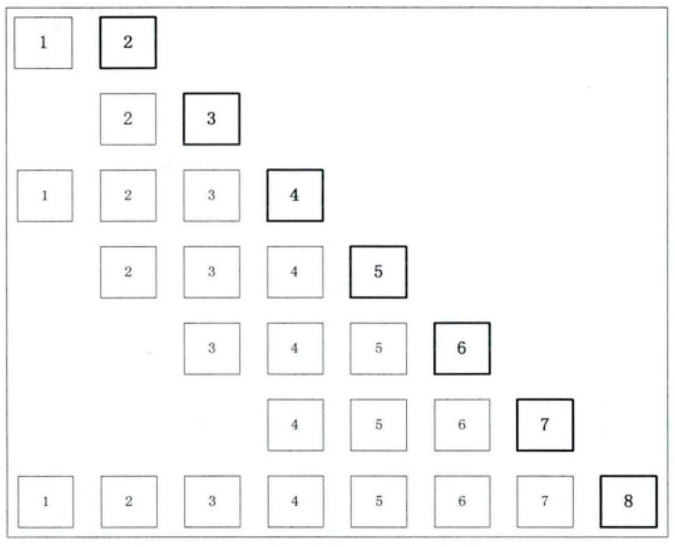
Online multiscale correction is based on the multiscale re-correction of binary length window data, as shown in Figure 1 [21]. The sliding window wavelet denoising method can be summarized as follows:
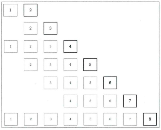
Figure 1.
Schematic diagram of the online multiscale (OLMS) sliding window.
- Step 1
- Use wavelet decomposition to decompose the data within the window of length.
- Step 2
- Use threshold wavelet denoising to reconstruct the signal.
- Step 3
- The last data point of the offline data is reserved for online use.
- Step 4
- When new measurement data is available, the window is moved in time to contain the latest measurement data while maintaining the maximum binary window length.
3.2. Offline Data Modeling Based on the SWWD-GLPP
Consider that there will be various interferences in the industrial process, and the sensor will also have measurement noise. If you directly model the data, there may be larger errors.In order to solve the noise problem, wavelet threshold denoising is performed on the data in the modeling stage to reduce the influence of noise on the model. The specific process of this article is shown in Figure 2, including three main parts: offline data modeling, online monitoring, and fault diagnosis.
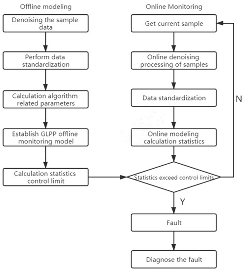
Figure 2.
Sliding window wavelet denoising-global local preserving projections (SWWD-GLPP) flow chart.
Step1: Assuming that there is a set of offline training data , the offline data matrix after wavelet threshold denoising is standardized, and the processed data is .
Step2: The GLPP algorithm contains many parameters; these parameters often affect the final effects of the algorithm, which makes it very important to choose the right parameters.In the GLPP algorithm, the value of has a great influence on the monitoring results. This paper uses Formula (23) to determine the value of :
where represents the trace of the matrix. , , , and can be obtained by the method in Section 2.3. In addition to finding , according to Formula (23), other methods or adjustments can be made according to the actual situation.
Step3: After determining the parameters, use the denoised data to establish a monitoring model based on the GLPP. The specific modeling method is shown in Formula (24):
where represents the residual matrix, and represents the matrix after projection.
Step4: Using Formulas (25) and (26), calculate the and statistics of the offline training data sample and form a dataset.
where is the sample of in Formula (23), which is different from the PCA, where represents the inverse of the diagonal matrix with eigenvalues arranged from small to large.
where is the residual vector of the th sample, and represents the value of the statistics of the th sample.
Step5: Determine the control limits
In order to determine whether the process is running under normal operating conditions, the control limits of the and statistics must be calculated. When the value of the statistics calculated by the online collected data is greater than the control limit, it is considered that a fault has occurred. This paper uses the kernel density estimation method to determine the control limit of each monitoring statistic [20]. The kernel density estimation method needs to obtain the monitoring statistics of the offline processing data first and then set the confidence limit. Compared with the traditional control limit determination method, the kernel density estimation method can track the distribution of data more closely, and the scope of application is wider.
where is the smoothing parameter, is the number of observations, is the kernel function (non-negative, conforms to the nature of probability density, and has a mean value of 0). In general, Gaussian kernel function is used:
Finally, the calculated control limits are marked as and .
3.3. Online Monitoring
Step1: Collect online data, use the sliding window wavelet denoising method in Section 2.1 to denoise, and the standardized data is .
Step2: Use the projection matrix obtained in the offline process and use the newly collected data to establish the following online monitoring model based on GLPP:
where is the vector after projection, is the residual vector of the online model, and is the projection matrix, which can be obtained by Formula (11).
Step3: Calculatethe and statistics.
where represents the diagonal matrix in which the eigenvalues are arranged from small values to large values.
Step4: Detection failure
By comparing with the control limits determined in the offline modeling, it is judged whether the process fails. Generally, there are two judgment methods. The first is the most commonly used method. As long as one of the two statistics exceeds the control limit, it is judged as a fault. This method of judgment can increase the sensitivity of the diagnosis, but it often leads to a high false report rate. The other method is to determine that a failure occurs only when both statistics fail. This method will greatly reduce the false report rate. The other method is to determine that a fault occurs only when both statistics are faulty. This method will greatly reduce the false report rate. The final accuracy of fault monitoring is the ratio of the number of detected faults in the fault data to the total number of faults, and the false alarm rate of fault monitoring is the ratio of the number of samples that are falsely reported as faults in the normal data samples to the number of normal samples.
Step5: Diagnose the fault
After the fault is detected, the abnormal variables in the data can be found by the method of a contribution graph, so as to determine the cause of the failure [26].
where is the number of principal components, and represents the contribution value of statistics at the th sample.
where represents the residual value of the th element, and represents the contribution value of the statistics at the th sample.
4. Simulation Process
4.1. Numerical Case
This section uses a simple mathematical case to prove the improvement of data monitorability after the use of sliding window denoising. For the convenience of viewing, a two-dimensional data set is used. First, set to be the normal distributed random data with 5 as the mean and 2 as the variance and to be the normally distributed random data with 1 as the mean and 1 as the variance. Both and contain 300 sets of data, and both contain gaussian noise. In the 101th sample of data, a random fault disturbance with a mean of 1 and a variance of 0.5 is introduced.
Figure 3 shows the data scatter diagram under the two processing methods, in which the red circle represents the normal data, and the blue cross represents the fault data. It can be found that the normal data and fault data of the unprocessed data (Figure 3a) are partly intertwined. This part of the data is often difficult to distinguish its true state during subsequent processing, resulting in a decrease in accuracy or an increase in the false alarm rate. After the data is processed by sliding window wavelet denoising (Figure 3b), we can clearly see the good separation of normal and fault data, which is obviously beneficial to the subsequent fault monitoring and fault diagnosis and, also, proves the effectiveness of our method.
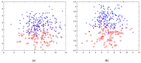
Figure 3.
(a) Scatter plot of unprocessed data. (b) Scatter plot of sliding window wavelet denoising processing data.
4.2. TE Simulation Process
The TE simulation process is widely used because of its complicated reaction process and production structure.It has 21 types of faults. For detailed information, please refer to the literature [27] and select 33 variables among them as monitoring variables [28]. In the stage of offline modeling, the denoising offline samples are used to build process monitoring models of PCA, GLPP, and SWWD-GLPP.In the online monitoring stage, the sliding window wavelet denoising method is used to denoise the online samples. The confidence limit of all algorithms is 99%.
Use PCA, GLPP, and SWWD-GLPP, the three process monitoring methods, to monitor 21 faults in the TE process and calculate the accuracy of the corresponding fault monitoring, as shown in Table 1. Since past research has proven that, in the TE processing data, fault 3, fault 9, and fault 15 are difficult to detect [27], the same situation is also in our experiment, so these three faults are not considered, and these three fault types are excluded from the table. In Table 1, the best performing indicators are marked in bold black.Obviously, the SWWD-GLPP method is better than the other two methods in most types of faults, especially for fault 11, fault 18, and fault 20. The accuracy of the monitoring is greatly improved.Although the performance of some fault types is not as good as the two methods compared, such as fault 1, fault 2, and fault 10, the differences can be found to be very small.At the end, we averaged the results of all fault monitoring quasi-removal rates, and it is obvious that the comprehensive situation of SWWD-GLPP proposed in this paper is better than PCA and GLPP.

Table 1.
Monitoring accuracy rate of the faults (%). PCA: principal component analysis and SWWD-GLPP: sliding window wavelet denoising-global local preserving projections. SPE: squared prediction error. Bold numbers: the best indicator results of all the methods.
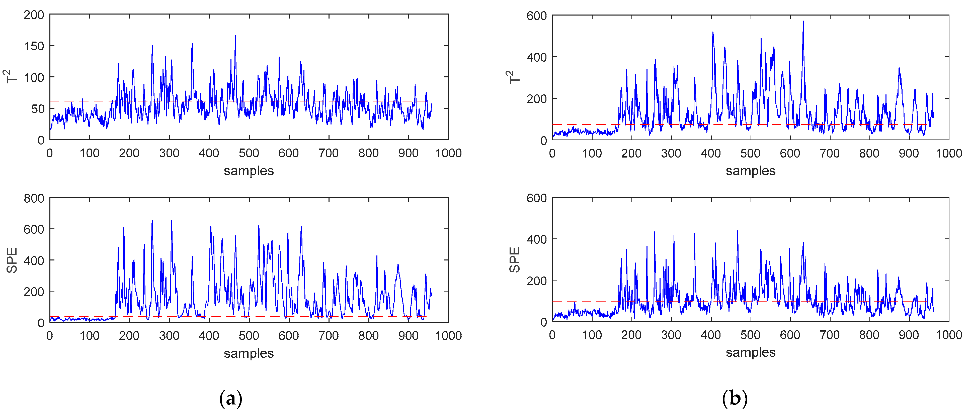
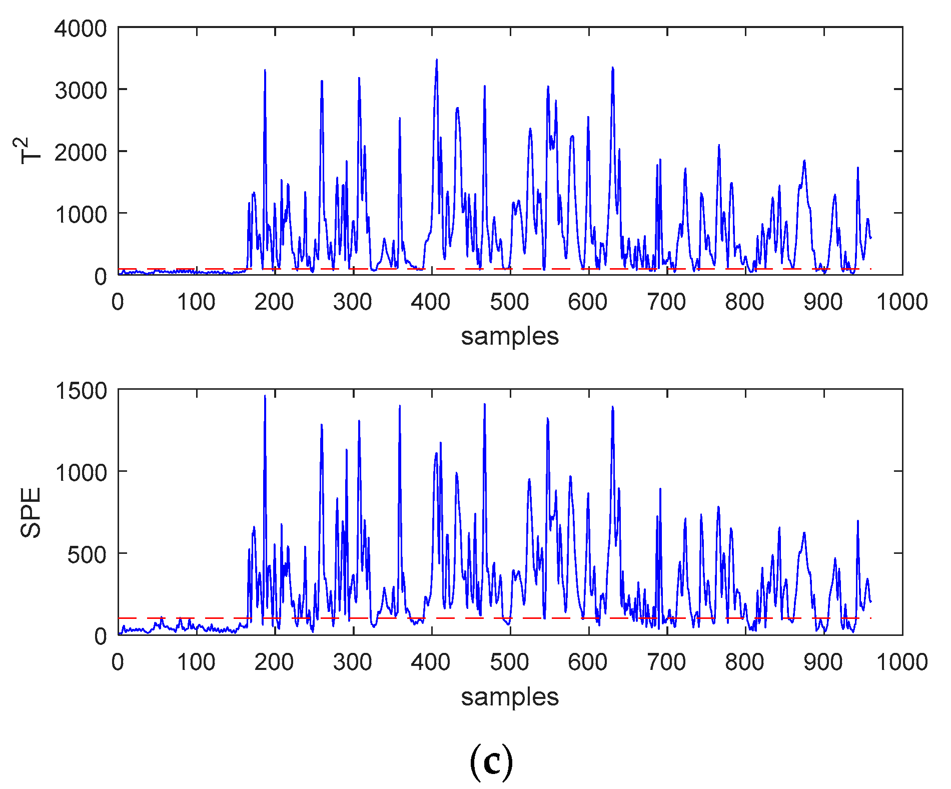
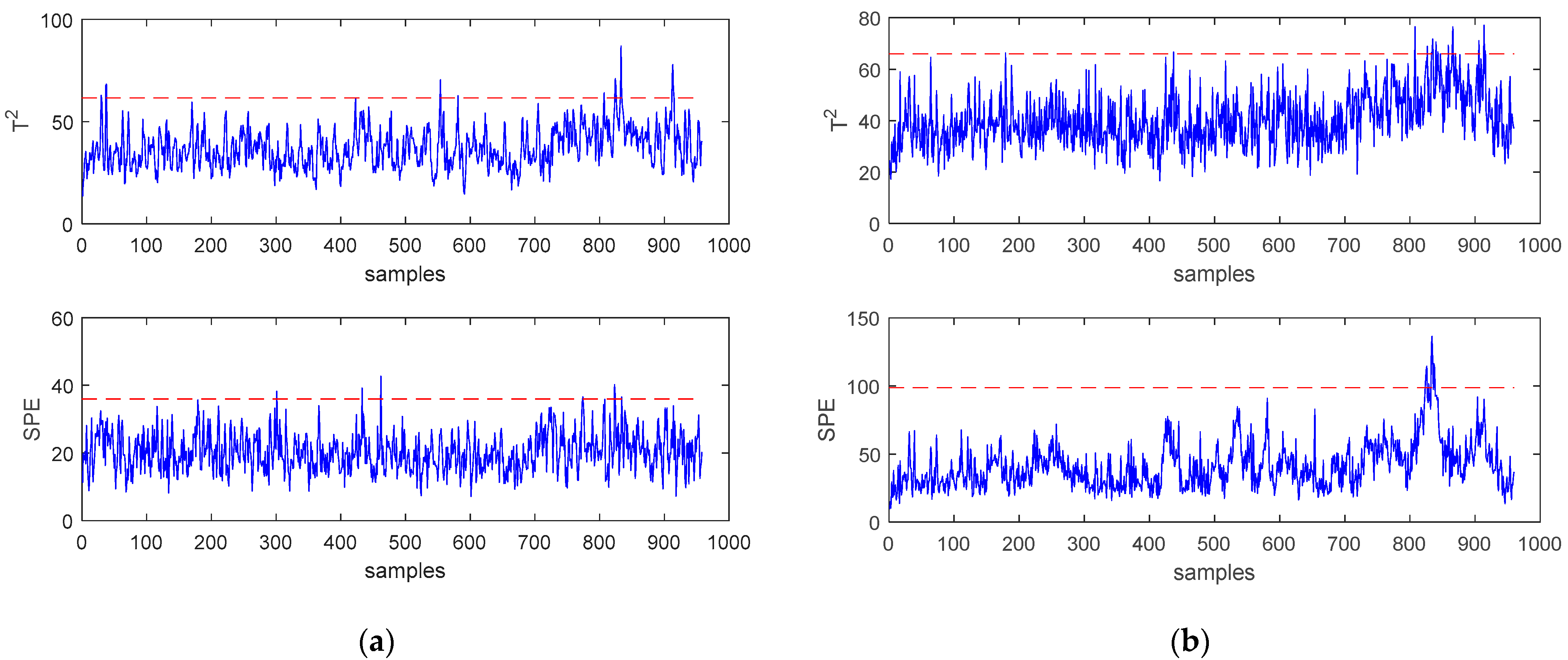
In order to more intuitively reflect the superiority of SWWD-GLPP compared to the other two methods, the monitoring results of fault 11 and fault 16 are shown in Figure 4 and Figure 5, respectively. For fault 11, it can be found that the statistics of the PCA method missed most of the faults. The two statistics of SWWD-GLPP and GLPP are better to detect the fault, and the effect of SWWD-GLPP is better.For fault 16, the two monitoring statistics of the PCA method failed to detect the fault well, while the statistics of SWWD-GLPP and GLPP detected the fault, and the SPE statistics performed generally.
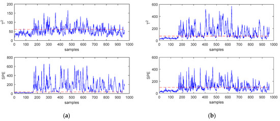
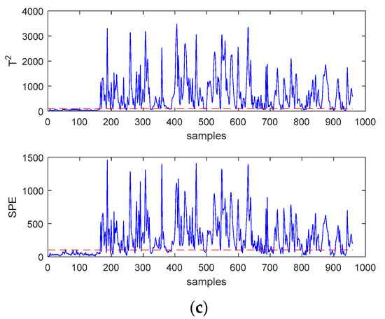
Figure 4.
(a) Monitoring charts of the principal component analysis (PCA) for fault 11. (b) Monitoring charts of GLPP for fault 11. (c) Monitoring charts of SWWD-GLPP for fault 11.
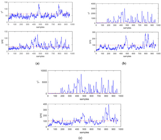
Figure 5.
(a) Monitoring charts of PCA for fault 16. (b) Monitoring charts of GLPP for fault 16. (c) Monitoring charts of SWWD-GLPP for fault 16.
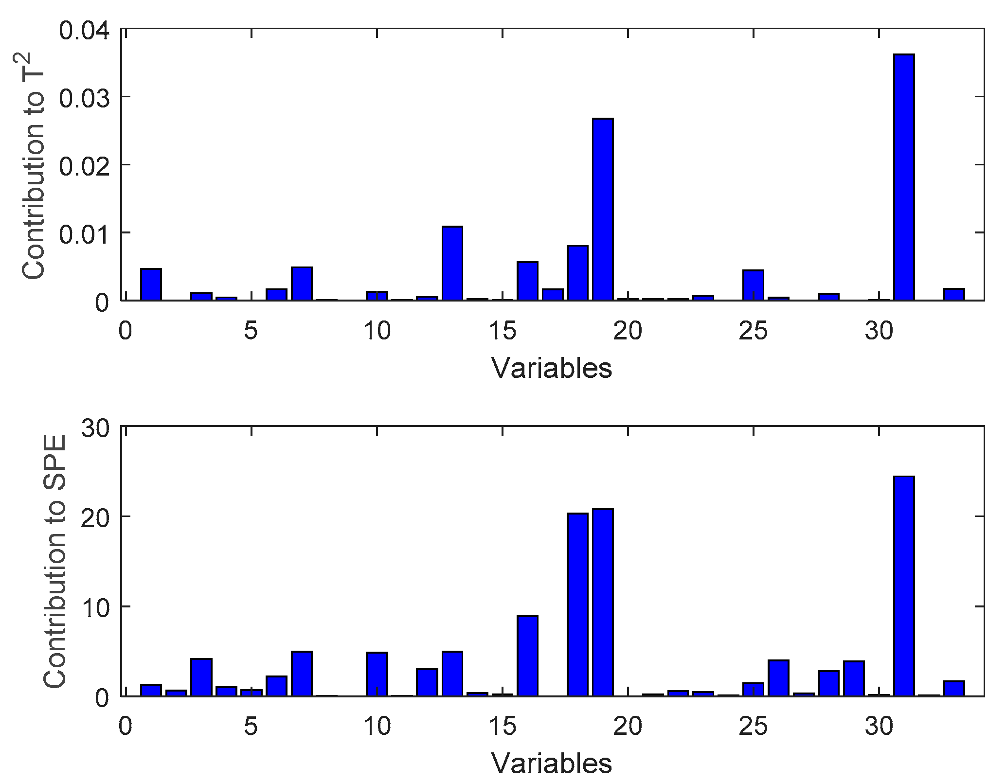
After the fault is detected, the contribution diagram method can be used to determine the cause of the fault. This article uses fault 10 of the TE process as the test sample. From Figure 6, it can be found that the largest cause of the fault is variable 31.
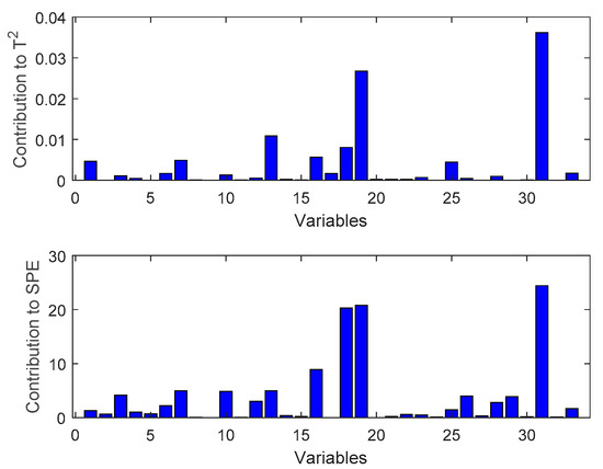
Figure 6.
Fault diagnosis diagram of fault 10.
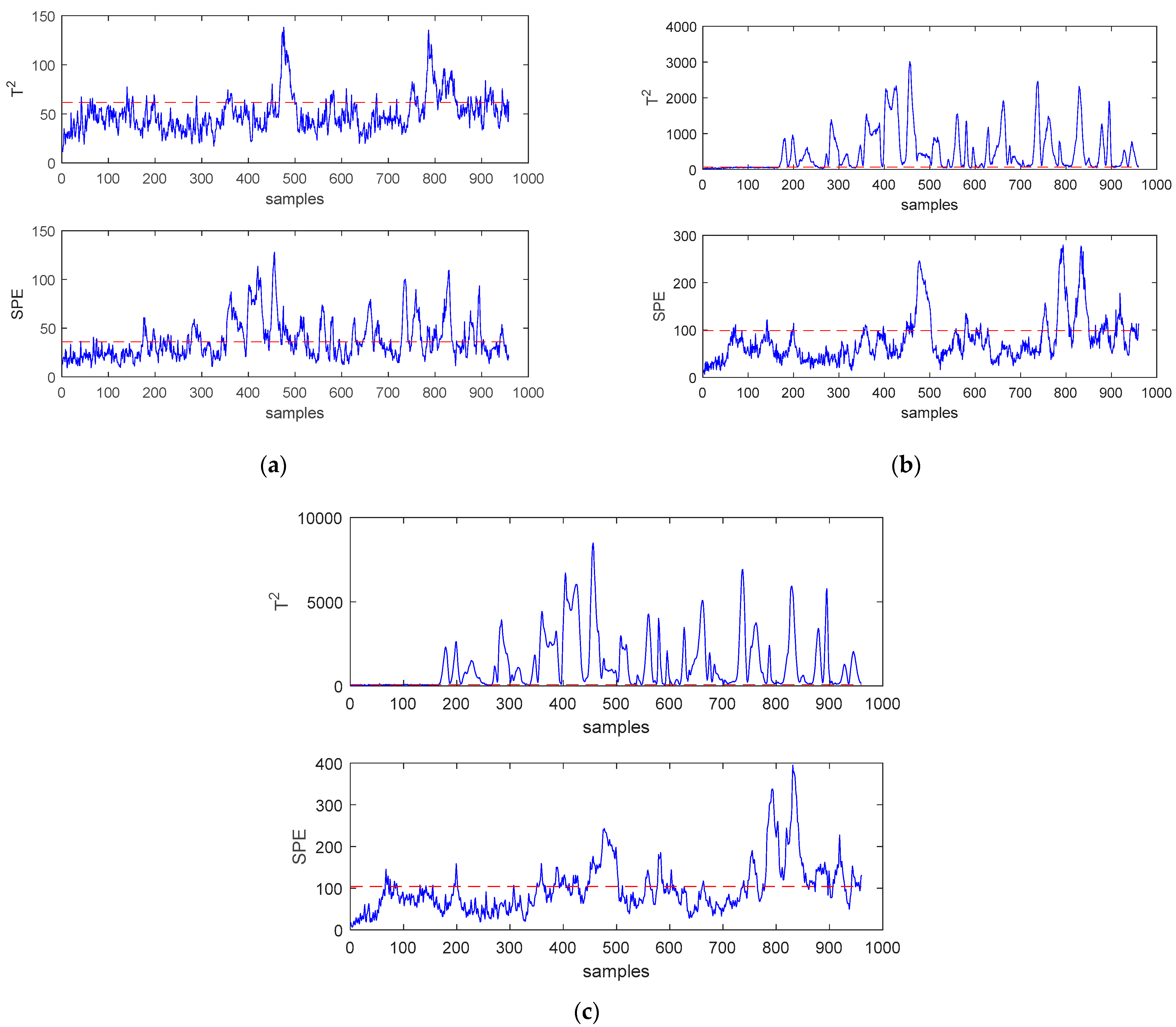
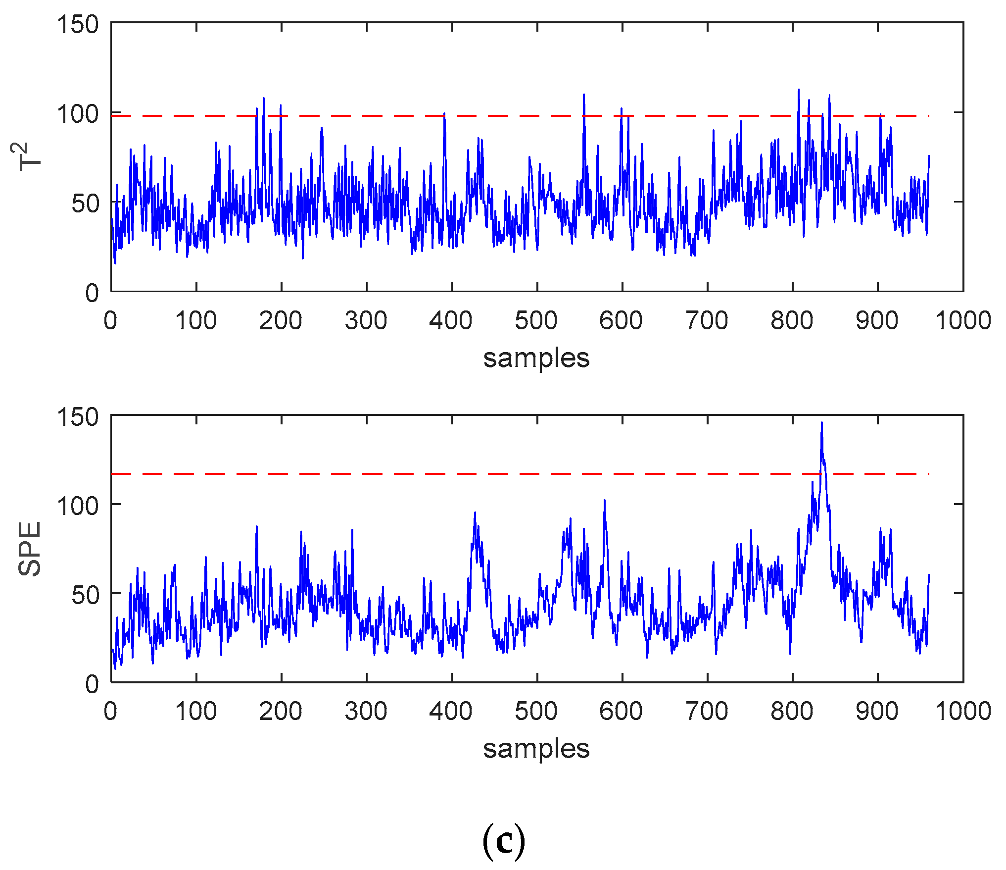
In process monitoring, the performance of the false alarm rate is also very important, because if the false alarm rate is too high, even with a high accuracy rate, it is often unusable. This article uses the nonfaulty test data provided in the TE dataset as the test sample. The monitoring statistics are shown in Figure 7, and the results of the false alarm rate are shown in Table 2. It can be found that the proposed SWWD-GLPP method has a lower false alarm rate. Combining the results of Table 1 and Table 2 can prove the effectiveness and superiority of the method proposed in this paper.
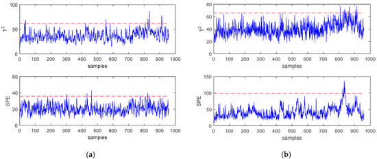
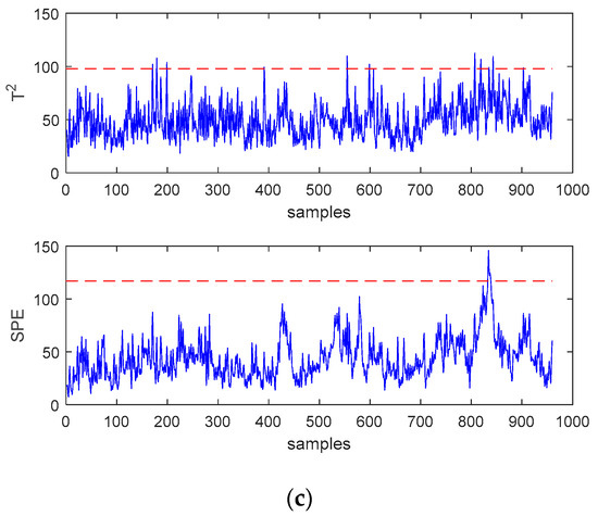
Figure 7.
(a) Monitoring charts of PCA for normal data. (b) Monitoring charts of GLPP for normal data. (c) Monitoring charts of SWWD-GLPP for normal data.

Table 2.
False alarm rates of normal data (%).
5. Conclusions
Aiming at the noise problem in industrial process measurement data, a sliding window denoising method is proposed, which makes wavelet denoising applicable to the online processing of processing data.In the offline phase, the wavelet denoising method is first used to denoise the offline data, and then, GLPP is used for offline modeling, and then, the control limit is obtained by the kernel density estimation method. In the online phase, the sliding window wavelet denoising method is used to denoise the online data in real time. Then, we used the model of the GLPP method to find the statistics, compare with the control limit, judge the fault situation, and diagnose the cause of the fault.The simulation study of the TE process fully shows that the SWWD-GLPP method is better than the traditional PCA and GLPP methods. However, SWWD-GLPP is still a monitoring method for linear data, and applying it to nonlinear processes is a problem that needs to be solved in subsequent research.
Author Contributions
The idea of this paper is put forward by F.Y., who is also responsible for method and analysis. Samples were prepared and analyzed by F.Y. The first draft was prepared by F.Y., reviewed and edited by Y.C., F.W. and R.Z. All authors have read and agreed to the published version of the manuscript.
Funding
This research received no external funding.
Institutional Review Board Statement
Not applicable.
Informed Consent Statement
Not applicable.
Data Availability Statement
Publicly available datasets were analyzed in this study. This data can be found here: https://github.com/camaramm/tennessee-eastman-profBraatz.
Conflicts of Interest
The authors declare no conflict of interest.
References
- Ge, Z.; Song, Z.; Gao, F. Review of Recent Research on Data-Based Process Monitoring. Ind. Eng. Chem. Res. 2013, 52, 3543–3562. [Google Scholar] [CrossRef]
- Jiang, X.; Zhao, H.; Leung, H. Fault Detection and Diagnosis in Chemical Processes Using Sensitive Principal Component Analysis. Ind. Eng. Chem. Res. 2013, 52, 1635–1644. [Google Scholar] [CrossRef]
- Bakshi, B.R. Multiscale PCA with application to multivariate statistical process monitoring. AIChE J. 1998, 44, 1596–1610. [Google Scholar] [CrossRef]
- Wang, J.; He, Q.P. Multivariate Statistical Process Monitoring Based on Statistics Pattern Analysis. Ind. Eng. Chem. Res. 2010, 49, 7858–7869. [Google Scholar] [CrossRef]
- Zhang, K.; Hao, H.; Chen, Z.; Ding, S.X.; Peng, K. A comparison and evaluation of key performance indicator-based multivariate statistics process monitoring approaches. J. Process. Control 2015, 33, 112–126. [Google Scholar] [CrossRef]
- Zhang, M.; Ge, Z.; Song, Z.; Fu, R. Global–Local Structure Analysis Model and Its Application for Fault Detection and Identification. Ind. Eng. Chem. Res. 2011, 50, 6837–6848. [Google Scholar] [CrossRef]
- Nomikos, P.; MacGregor, J.F. Monitoring batch processes using multiway principal component analysis. AIChE J. 1994, 40, 1361–1375. [Google Scholar] [CrossRef]
- Nomikos, P.; MacGregor, J.F. Multi-way partial least squares in monitoring batch processes. Chemom. Intell. Lab. Syst. 1995, 30, 97–108. [Google Scholar] [CrossRef]
- Kano, M.; Tanaka, S.; Hasebe, S.; Hashimoto, I.; Ohno, H. Monitoring independent components for fault detection. AIChE J. 2003, 49, 969–976. [Google Scholar] [CrossRef]
- Choi, S.W.; Lee, C.; Lee, J.-M.; Park, J.H.; Lee, I.-B. Fault detection and identification of nonlinear processes based on kernel PCA. Chemom. Intell. Lab. Syst. 2005, 75, 55–67. [Google Scholar] [CrossRef]
- Zhang, Y.; Zhou, H.; Qin, S.J.; Chai, T. Decentralized Fault Diagnosis of Large-Scale Processes Using Multiblock Kernel Partial Least Squares. IEEE Trans. Ind. Inform. 2009, 6, 3–10. [Google Scholar] [CrossRef]
- Zhang, Y.; An, J.; Zhang, H. Monitoring of time-varying processes using kernel independent component analysis. Chem. Eng. Sci. 2013, 88, 23–32. [Google Scholar] [CrossRef]
- He, X.F.; Niyogi, P. Locality preserving projections. In Proceedings of the Conference on Advances in Neural Information Processing Systems, Vancouver, BC, Canada, 8−13 December 2003; MIT Press: Cambridge, MA, USA, 2004. [Google Scholar]
- Fezai, R.; Mansouri, M.; Taouali, O.; Harkat, M.F.; Bouguila, N. Online reduced kernel principal component analysis for process monitoring. J. Process. Control 2018, 61, 1–11. [Google Scholar] [CrossRef]
- Hu, K.; Yuan, J. Multivariate statistical process control based on multiway locality preserving projections. J. Process. Control 2008, 18, 797–807. [Google Scholar] [CrossRef]
- Luo, L. Process Monitoring with Global–Local Preserving Projections. Ind. Eng. Chem. Res. 2014, 53, 7696–7705. [Google Scholar] [CrossRef]
- Luo, L.; Bao, S.; Mao, J.; Tang, D. Nonlinear process monitoring based on kernel global-local preserving projections. J. Process Control 2016, 38, 11–21. [Google Scholar] [CrossRef]
- Tang, Q.; Chai, Y.; Qu, J.; Fang, X. Industrial process monitoring based on Fisher discriminant global-local preserving projection. J. Process Control 2019, 81, 76–86. [Google Scholar] [CrossRef]
- Donoho, D.L. Denoising by soft-thresholding. IEEE Trans. Inf. Theory 1995, 41, 613–627. [Google Scholar] [CrossRef]
- Martin, E.; Morris, A. Non-parametric confidence bounds for process performance monitoring charts. J. Process. Control 1996, 6, 349–358. [Google Scholar] [CrossRef]
- Nounou, M.N.; Bakshi, B.R. On-line multiscale filtering of random and gross errors without process models. AIChE J. 1999, 45, 1041–1058. [Google Scholar] [CrossRef]
- Qin, S.J.; Dunia, R. Determining the number of principal components for best reconstruction. J. Process Control 2000, 10, 245–250. [Google Scholar] [CrossRef]
- Kruger, U.; Xie, L. Advances in statistical monitoring of complex multivariate processes. J. Qual. Technol. 2012, 45, 118–119. [Google Scholar]
- Belkin, M.; Niyogi, P. Laplacian Eigenmaps for Dimensionality Reduction and Data Representation. Neural Comput. 2003, 15, 1373–1396. [Google Scholar] [CrossRef]
- Rowei, S.T.; Saul, L.K. Nonlinear dimensionality reduction by locally linear embedding. Science 2000, 290, 2323–2326. [Google Scholar] [CrossRef] [PubMed]
- McAvoy, T. Fault Detection and Diagnosis in Industrial Systems. J. Process. Control 2002, 12, 453–454. [Google Scholar] [CrossRef]
- Chiang, L.H.; Russell, E.L.; Braatz, R.D. Fault Detection and Diagnosis in Industrial Systems; Springer Science and Business Media LLC: London, UK, 2001. [Google Scholar]
- Tong, C.; Palazoglu, A.; Yan, X. Improved ICA for process monitoring based on ensemble learning and Bayesian inference. Chemom. Intell. Lab. Syst. 2014, 135, 141–149. [Google Scholar] [CrossRef]
Publisher’s Note: MDPI stays neutral with regard to jurisdictional claims in published maps and institutional affiliations. |
© 2021 by the authors. Licensee MDPI, Basel, Switzerland. This article is an open access article distributed under the terms and conditions of the Creative Commons Attribution (CC BY) license (http://creativecommons.org/licenses/by/4.0/).

