Snapse: A Visual Tool for Spiking Neural P Systems

Abstract
:1. Introduction
2. Preliminaries
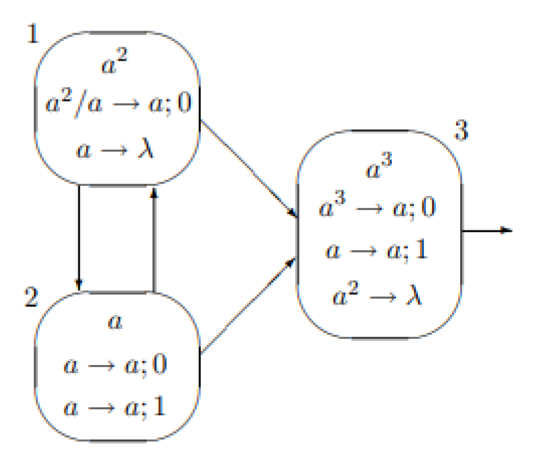
2.1. Spiking Neural P Systems
- 1.
- O = {a} is the singleton alphabet (a is called spike);
- 2.
- are neurons, of the form where:
- (a)
- is the initial number of spikes contained in ;
- (b)
- is a finite set of rules of the following two forms:
- i.
- , where E is a regular expression over and ;
- ii.
- , with the restriction that for each rule of type (i) from , we have a ;
- 3.
- with for all () (synapses between neurons);
- 4.
- in, out indicate the input and the output neurons, respectively.
2.2. Spiking Neural P Systems with Extended Rules
- 1.
- O = {a} is the singleton alphabet (a is called spike);
- 2.
- are neurons, of the form where:
- (a)
- is the initial number of spikes contained in ;
- (b)
- is a finite set of rules of the form , where E is a regular expression over , , and with the restriction that ;
- 3.
- with for all () (synapses between neurons);
- 4.
- indicate the output neuron .
2.3. Matrix Representation of an SN P System
2.4. Further Representations of SN P Systems
3. Snapse: A Graphical User Interface for Simulating and Creating Spiking Neural P Systems
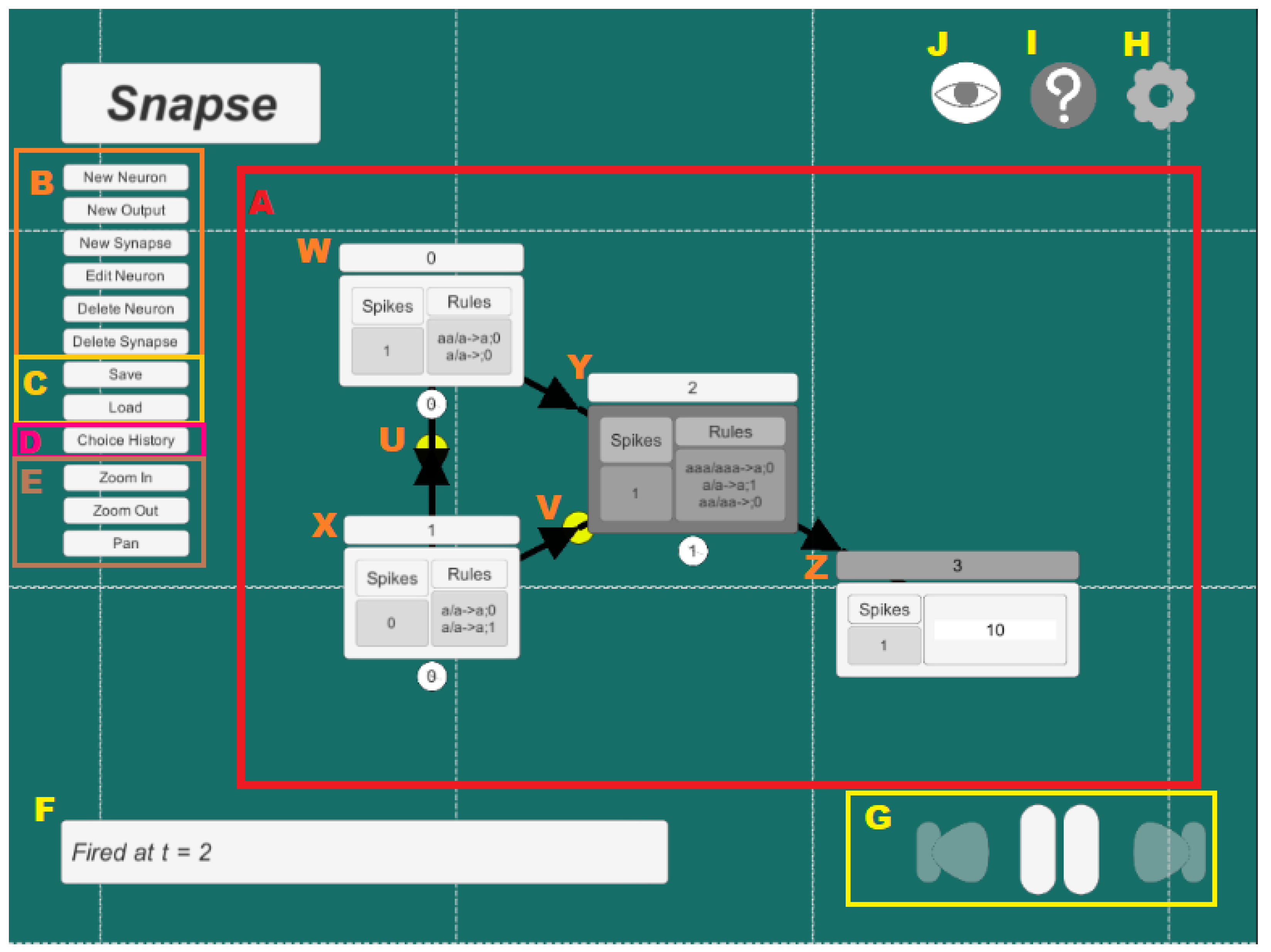
3.1. Basic Functionalities and Limitations
- Workspace (labelled A): contains the entire SN P system.
- Neuron Editing Options (labelled B): contains all the buttons that are useful in modifying the SN P systems. This includes adding new neurons, output neurons, and synapses; removing neurons and synapses; modifying rules and spikes for each neuron.
- Saving and Loading (labeled C): contains buttons to save and load work.
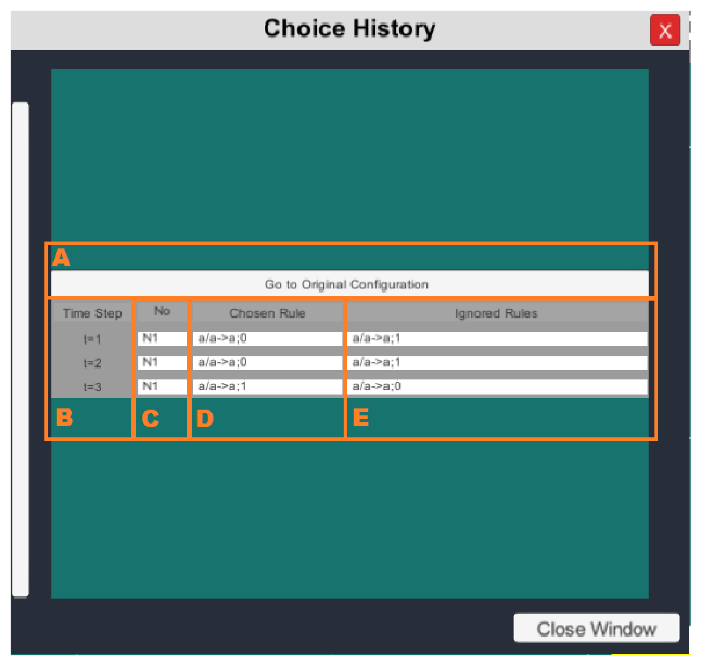
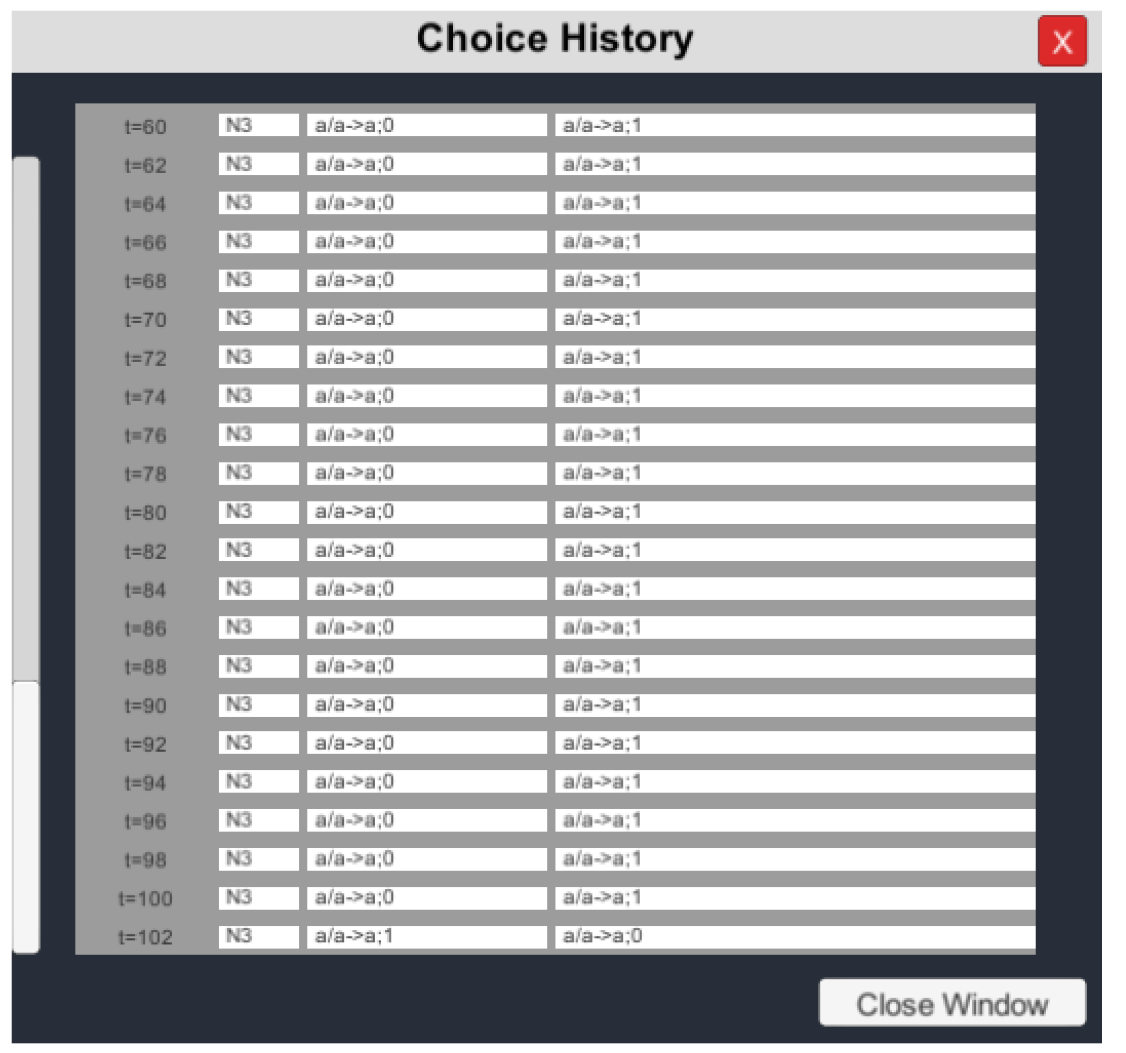
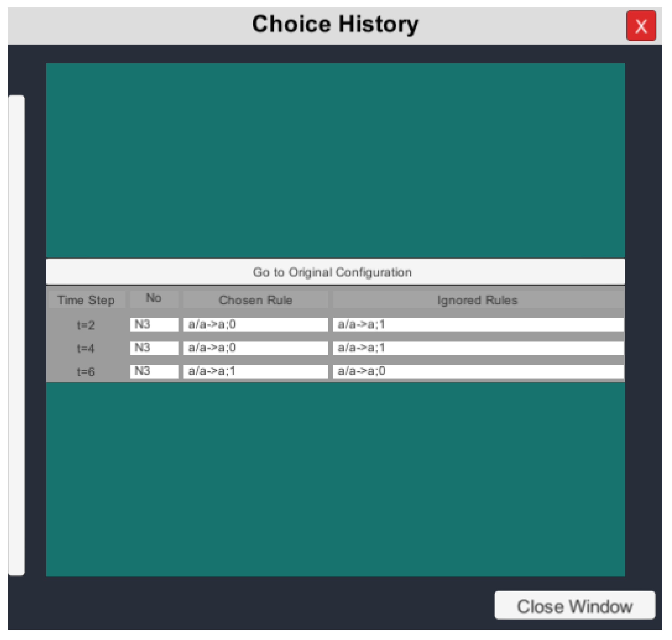
- Choice History Window (labelled D): Opens the choice history window which lists all non-deterministic choices made.
- Viewing Options (labelled E): contains all the buttons that help in navigating through the SN P System. This includes panning, zooming in and out.
- Status Indicators (labelled F): a status bar that shows through text the current process undertaken by the program.
- Firing Options (labelled G): contains the buttons that control the firing of neurons. This includes continuous firing, moving forward one time step, and moving backward one time step.
- Settings (labelled H): Contains simulation modes and hide/view options for rules, labels, and animations.
- About/Help (labelled I): Contains useful information such as keyboard shortcuts and the output path.
- Hide interface (labelled J): Toggles the visibility of all unnecessary buttons surrounding the workspace to reduce clutter.
3.2. Neuron and Output Representation
3.3. Rule Syntax
3.4. Configuration Syntax
<name>{
- spikes = <int>:rules = {<rule1>, <rule2>,\dots, <rulen>}:outsynapses = [<name1>, <name2>, <name3>]:delay = <int>:storedGive = <int> <(default:0)>:storedConsume = <int> <(default:0)>:outputNeuron = <boolean>:position = (<float>,<float>,<float>) <(default: (0, 0, 0))>:}
3.5. Graphical User Interface
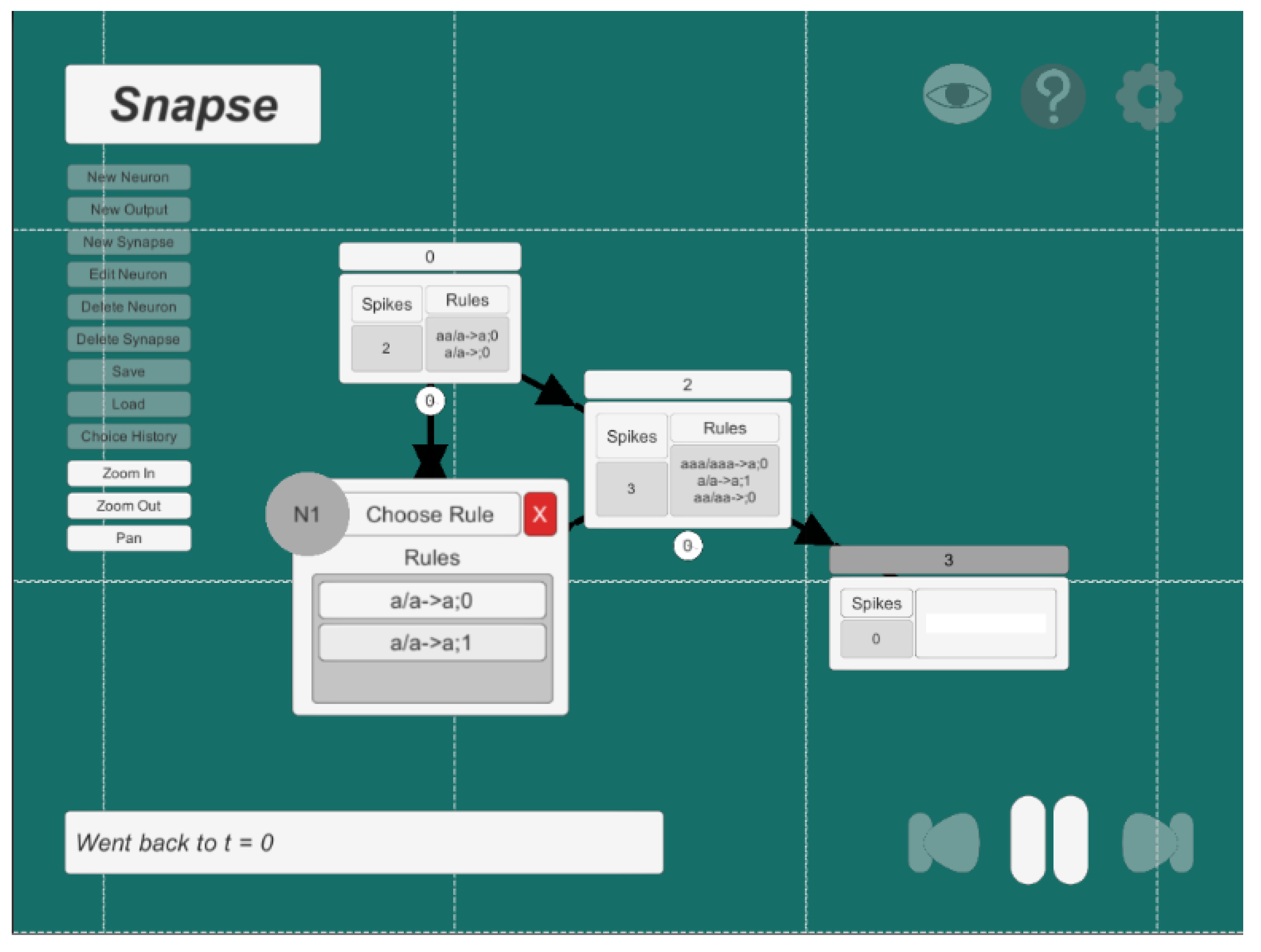
Choice History UI
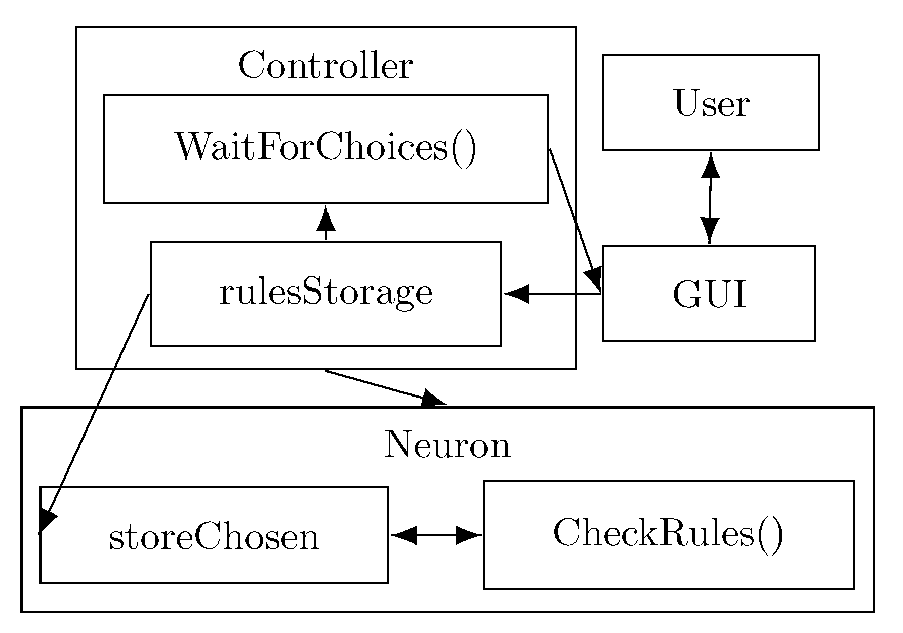
3.6. Architecture
3.7. Simulation Algorithm

4. Comparison with Other Tools
4.1. P-Lingua
4.2. JFLAP
4.3. Snoopy
4.4. MeCoSim
4.5. UPSimulator
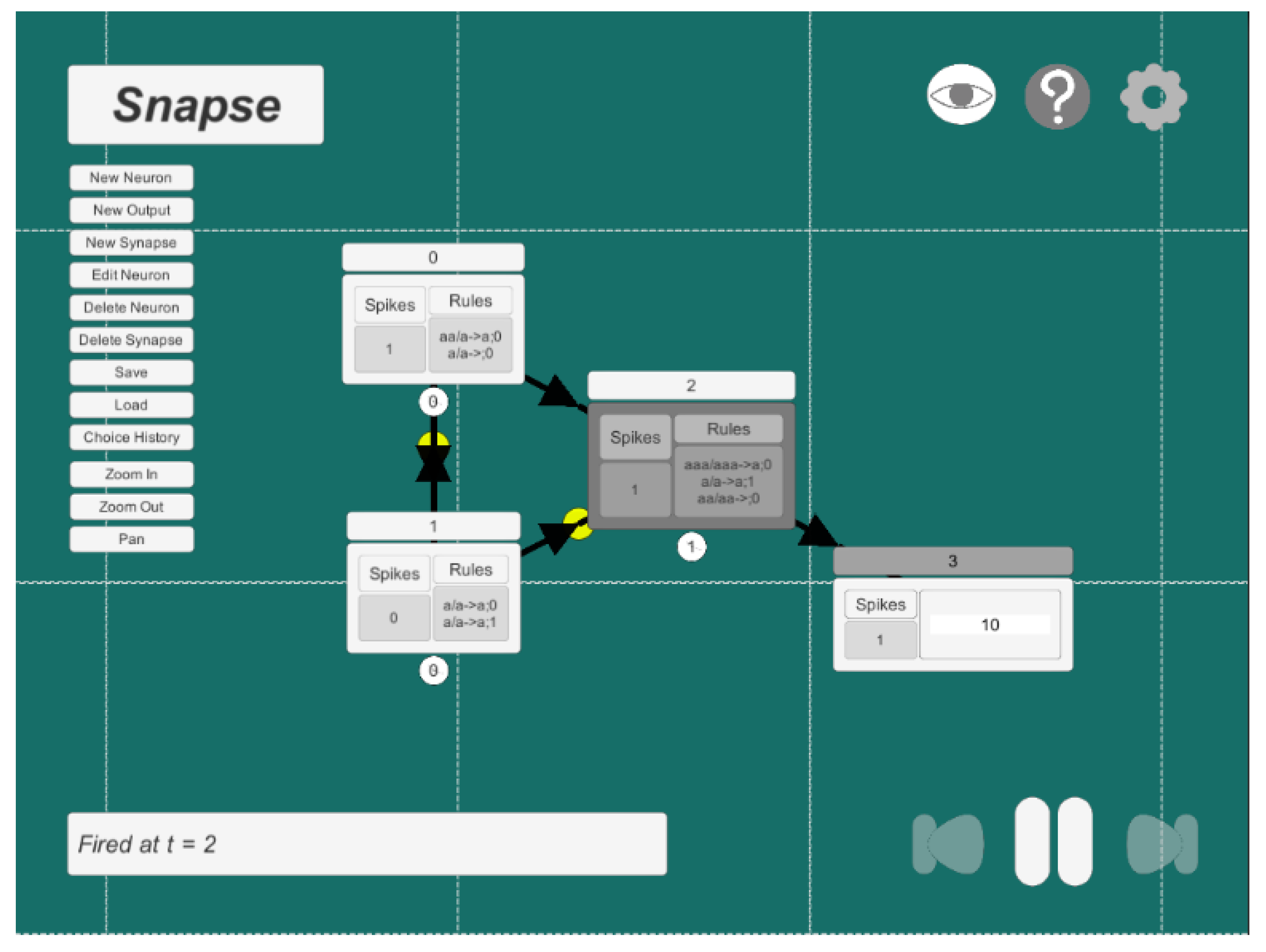
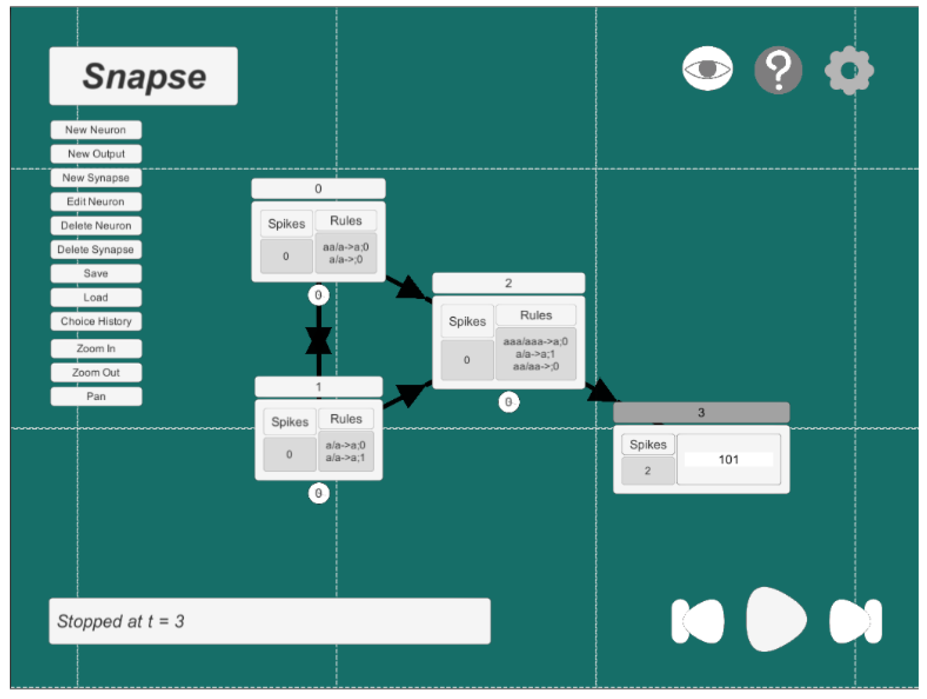
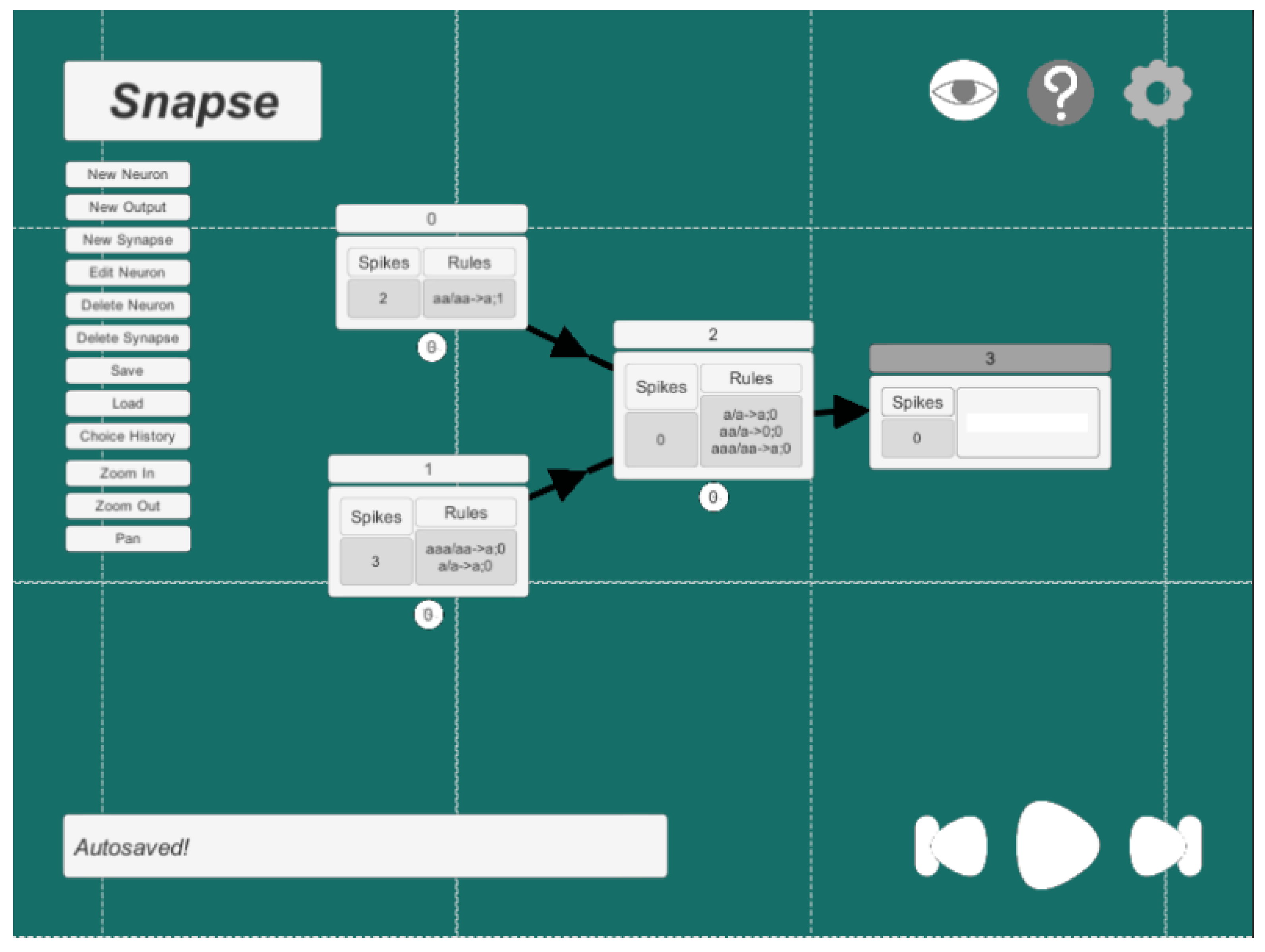
5. A Few Examples
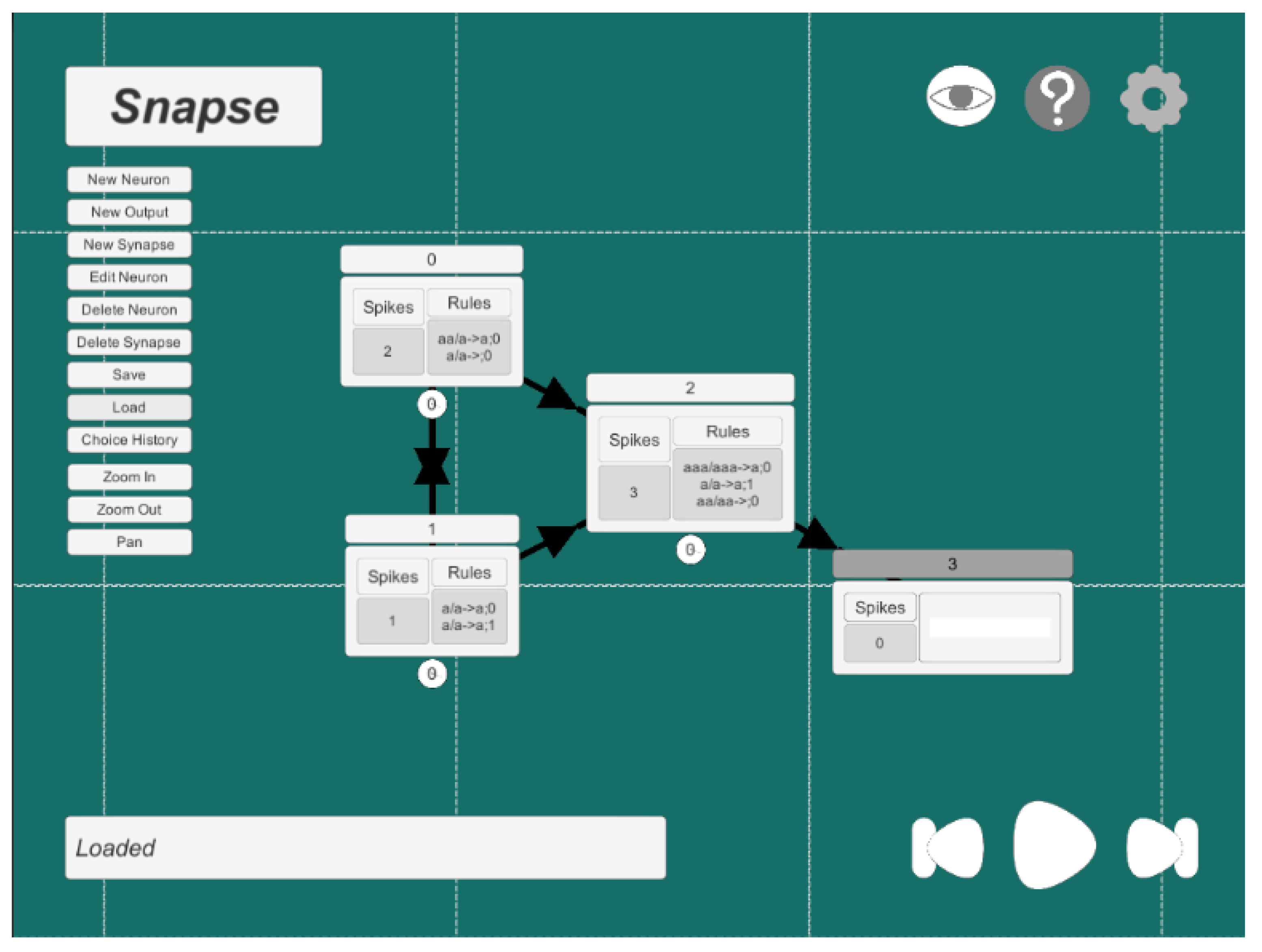
neurons = [N0, N1, N2, O3]:
- N0{spikes = 2:rules = {[aa/a->a;0], [a/a->0;0]}:outsynapses = [N1, N2]:delay = -1:storedGive = 0:storedConsume = 0:outputNeuron = False:position = <(-3,1.5,0)>:}N1{spikes = 1:rules = {[a/a->a;0], [a/a->a;1]}:outsynapses = [N0, N2]:delay = -1:storedGive = 0:storedConsume = 0:outputNeuron = False:position = <(-3,-1.5,0)>:}N2{spikes = 3:rules = {[aaa/aaa->a;0], [a/a->a;1], [aa/aa->0;0]}:outsynapses = [O3]:delay = -1:storedGive = 0:storedConsume = 0:outputNeuron = False:position = <(0,0,0)>:}N3{spikes = 0:rules = {[]}:outsynapses = []:delay = -1:storedGive = 0:storedConsume = 0:outputNeuron = True:storedReceived = 0:bitString = null:position = <(3,0,0)>:}
6. Final Remarks
Author Contributions
Funding
Acknowledgments
Conflicts of Interest
Appendix A. Examples of SN P Systems in Snapse
Appendix A.1. Example of an SN P System That Generates all Natural Numbers Greater than One in Snapse


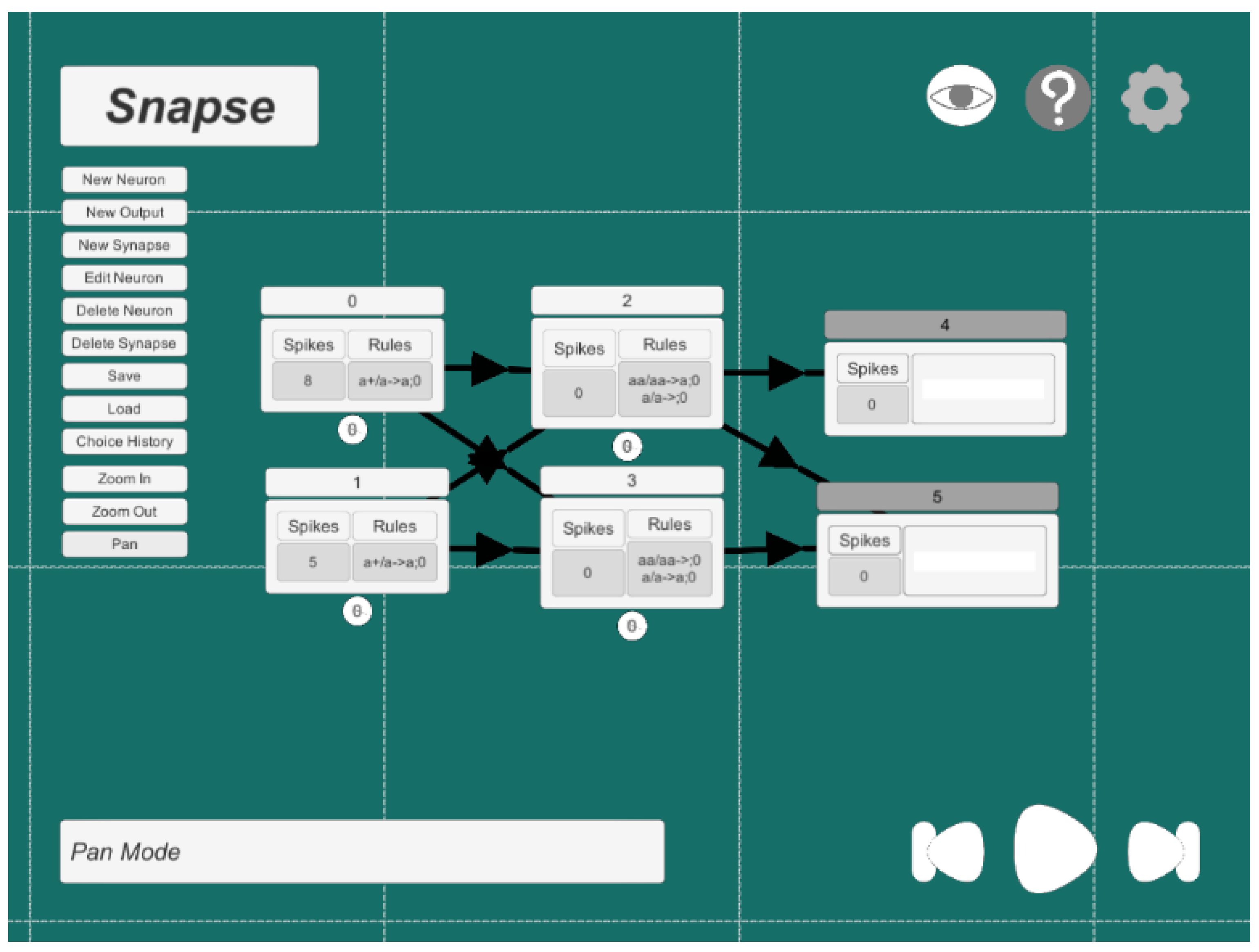
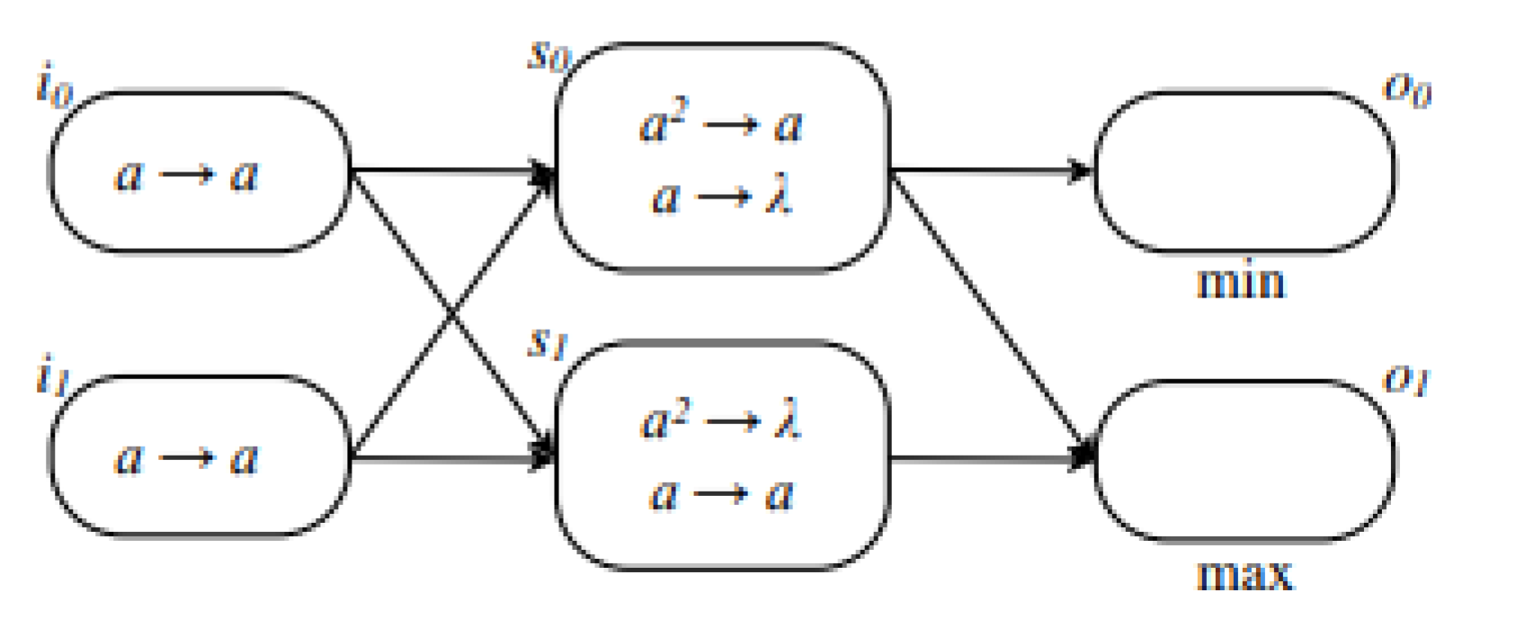
Appendix A.2. Graphical Representation of an Increasing Comparator

Appendix A.3. An Example of an Increasing Comparator in Snapse

Appendix A.4. An Example of a Configuration File of an Increasing Comparator in Snapse
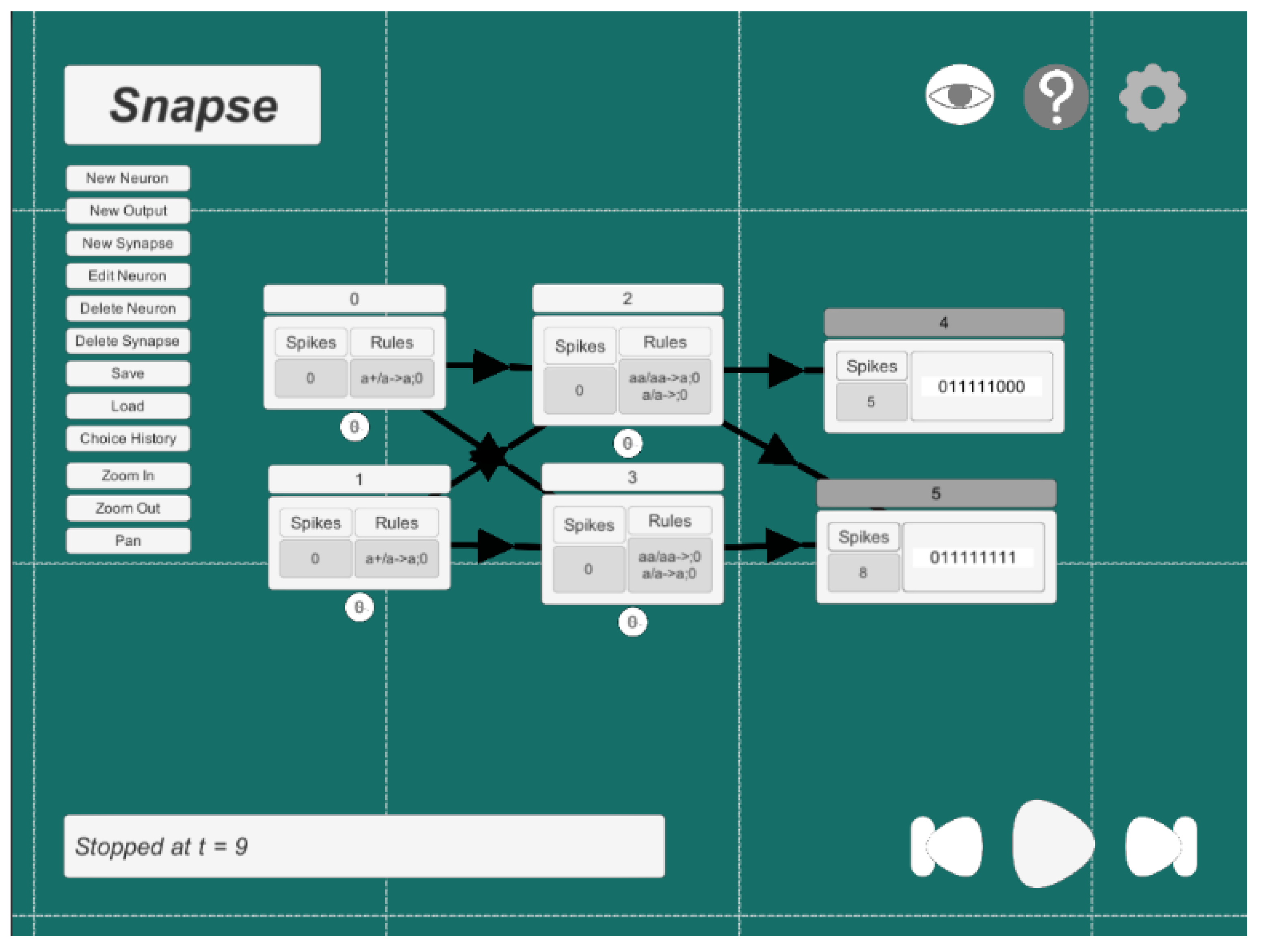
neurons = [N0, N1, N2, N3, O4, O5]:
- N0{spikes = 8:rules = {[a+/a->a;0]}:outsynapses = [N2, N3]:delay = 0:storedGive = 1:storedConsume = 1:outputNeuron = False:position = (-3,1,0):}N1{spikes = 5:rules = {[a+/a->a;0]}:outsynapses = [N2, N3]:delay = 0:storedGive = 1:storedConsume = 1:outputNeuron = False:position = (-3,-1,0):}N2{spikes = 0:rules = {[aa/aa->a;0], [a/a->0;0]}:outsynapses = [O4, O5]:delay = 0:storedGive = 1:storedConsume = 2:outputNeuron = False:position = (0,1,0):}N3{spikes = 0:rules = {[aa/aa->0;0], [a/a->a;0]}:outsynapses = [O5]:delay = 0:storedGive = 0:storedConsume = 2:outputNeuron = False:position = (0,-1,0):}N4{spikes = 0:rules = {[]}:outsynapses = []:delay = -4:storedGive = 0:storedConsume = 0:outputNeuron = True:storedReceived = 0:bitString = null:position = (3,1,0):}N5{spikes = 0:rules = {[]}:outsynapses = []:delay = -4:storedGive = 0:storedConsume = 0:outputNeuron = True:storedReceived = 0:bitString = null:position = (3,-1,0):}
Appendix A.5. An Example of a Bit Adder in Snapse


Appendix A.6. An Example of a Configuration File of a Bit Adder in Snapse
neurons = [N0, N1, N2, O3]:
- N0{spikes = 2:rules = {[aa/aa->a;1]}:outsynapses = [N2]:delay = 0:storedGive = 1:storedConsume = 2:outputNeuron = False:position = (-3,1,0):}N1{spikes = 3:rules = {[aaa/aa->a;0], [a/a->a;0]}:outsynapses = [N2]:delay = 0:storedGive = 1:storedConsume = 1:outputNeuron = False:position = (-3,-1,0):}N2{spikes = 0:rules = {[a/a->a;0], [aa/a->0;0], [aaa/aa->a;0]}:outsynapses = [O3]:delay = 0:storedGive = 1:storedConsume = 1:outputNeuron = False:position = (0,0,0):}N3{spikes = 0:rules = {[]}:outsynapses = []:delay = 0:storedGive = 0:storedConsume = 0:outputNeuron = True:storedReceived = 0:bitString = null:position = (3,0,0):}
References
- Păun, G. Computing with membranes. J. Comput. Syst. Sci. 2000, 61, 108–143. [Google Scholar] [CrossRef] [Green Version]
- Ionescu, M.; Păun, G.; Yokomori, T. Spiking Neural P Systems. Fundam. Inform. 2006, 71, 279–308. [Google Scholar]
- Calude, C.S.; Păun, G. Computing with Cells and Atoms: An Introduction to Quantum, DNA and Membrane Computing; Taylor & Francis/Hemisphere: Bristol, PA, USA, 2001. [Google Scholar]
- Păun, G. P Systems with Active Membranes: Attacking NP-Complete Problems. J. Autom. Lang. Comb. 2001, 6, 75–90. [Google Scholar]
- Ciobanu, G.; Păun, G.; Pérez-Jiménez, M.J. Applications of Membrane Computing; Springer: Berlin/Heidelberg, Germany, 2006; Volume 17. [Google Scholar]
- Frisco, P.; Gheorghe, M.; Pérez-Jiménez, M.J. Applications of Membrane Computing in Systems and Synthetic Biology; Springer: Berlin/Heidelberg, Germany, 2014. [Google Scholar]
- Paun, G.; Rozenberg, G.; Salomaa, A. The Oxford Handbook of Membrane Computing; Oxford University Press, Inc.: New York, NY, USA, 2010. [Google Scholar]
- Leporati, A.; Mauri, G.; Zandron, C.; Păun, G.; Pérez-Jiménez, M. Uniform solutions to SAT and Subset Sum by spiking neural P systems. Nat. Comput. 2009, 8, 681–702. [Google Scholar] [CrossRef]
- Cabarle, F.G.C.; Adorna, H.N.; Martínez del Amor, M.Á.; Pérez Jiménez, M.d.J. Improving GPU simulations of spiking neural P systems. Rom. J. Inf. Sci. Technol. 2012, 15, 5–20. [Google Scholar]
- Carandang, J.; Villaflores, J.M.B.; Cabarle, F.G.C.; Adorna, H.N.; Martínez-del Amor, M.A. CuSNP: Spiking neural P systems simulators in CUDA. Rom. J. Inf. Sci. Technol. 2017, 20, 57–70. [Google Scholar]
- Carandang, J.P.; Cabarle, F.G.C.; Adorna, H.N.; Hernandez, N.H.S.; Martínez-del Amor, M.Á. Handling non-determinism in spiking neural P systems: Algorithms and simulations. Fundam. Inform. 2019, 164, 139–155. [Google Scholar] [CrossRef]
- Aboy, B.C.D.; Bariring, E.J.A.; Carandang, J.P.; Cabarle, F.G.C.; Cruz, R.T.D.L.; Adorna, H.N.; Martínez-del-Amor, M.A. Optimizations in CuSNP Simulator for Spiking Neural P Systems on CUDA GPUs. In Proceedings of the 2019 International Conference on High Performance Computing Simulation (HPCS), Dublin, Ireland, 15–19 July 2019; pp. 535–542. [Google Scholar]
- Cabarle, F.G.C.; de la Cruz, R.T.A.; Cailipan, D.P.P.; Zhang, D.; Liu, X.; Zeng, X. On solutions and representations of spiking neural P systems with rules on synapses. Inf. Sci. 2019, 501, 30–49. [Google Scholar] [CrossRef]
- Ibarra, O.H.; Păun, A.; Păun, G.; Rodríguez-Patón, A.; Sosík, P.; Woodworth, S. Normal forms for spiking neural P systems. Theor. Comput. Sci. 2007, 372, 196–217. [Google Scholar] [CrossRef] [Green Version]
- Pan, L.; Păun, G. Spiking neural P systems: An improved normal form. Theor. Comput. Sci. 2010, 411, 906–918. [Google Scholar] [CrossRef] [Green Version]
- Macababayao, I.C.H.; Cabarle, F.G.C.; dela Cruz, R.T.A.; Adorna, H.N.; Zeng, X. Notes on Improved Normal Forms of Spiking Neural P Systems and Variants; Pre-Proc. In Proceedings of the Asian Conference on Membrane Computing (ACMC2019), Xiamen, China, 14–17 November 2019. [Google Scholar]
- Zeng, X.; Adorna, H.; Martínez-del Amor, M.; Pan, L.; Pérez-Jiménez, M. Matrix Representation of Spiking Neural P Systems. In Proceedings of the International Conference on Membrane Computing, Jena, Germany, 24–27 August 2010; Volume 6501, pp. 377–391. [Google Scholar]
- Verlan, S.; Freund, R.; Alhazov, A.; Ivanov, S.; Pan, L. A formal framework for spiking neural P systems. J. Membr. Comput. 2020, 2, 355–368. [Google Scholar] [CrossRef]
- Jimenez, Z.B.; Cabarle, F.G.C.; de la Cruz, R.T.A.; Buño, K.C.; Adorna, H.N.; Hernandez, N.H.S.; Zeng, X. Matrix representation and simulation algorithm of spiking neural P systems with structural plasticity. J. Membr. Comput. 2019, 1, 145–160. [Google Scholar] [CrossRef] [Green Version]
- Chen, H.; Freund, R.; Ionescu, M.; Păun, G.; Pérez-Jiménez, M.J. On string languages generated by spiking neural P systems. Fundam. Inform. 2007, 75, 141–162. [Google Scholar]
- Cabarle, F.G.C.; Adorna, H.N. On Structures and Behaviors of Spiking Neural P Systems and Petri Nets. In CMC 2012: Membrane Computing, Proceedings of the International Conference on Membrane Computing, Chişinău, Republic of Moldova, 20–23 August 2013; Springer: Berlin/Heidelberg, Germany, 2013; Volume 7762, pp. 145–160. [Google Scholar]
- Ibarra, O.H.; Pérez-Jiménez, M.J.; Yokomori, T. On spiking neural P systems. Nat. Comput. 2010, 9, 475–491. [Google Scholar] [CrossRef]
- Cabarle, F.G.C.; Adorna, H.N.; Pérez-Jiménez, M.J. Notes on spiking neural P systems and finite automata. Nat. Comput. 2016, 15, 533–539. [Google Scholar] [CrossRef] [Green Version]
- De la Cruz, R.T.A.; Cabarle, F.G.; Adorna, H.N. Generating context-free languages using spiking neural P systems with structural plasticity. J. Membr. Comput. 2019, 1, 161–177. [Google Scholar] [CrossRef] [Green Version]
- Adorna, H.N. Computing with SN P systems with I/O mode. J. Membr. Comput. 2020, 2, 230–245. [Google Scholar] [CrossRef]
- Rong, H.; Wu, T.; Pan, L.; Zhang, G. Spiking neural P systems: Theoretical results and applications. In Enjoying Natural Computing; Springer: Berlin/Heidelberg, Germany, 2018; pp. 256–268. [Google Scholar]
- Díaz-Pernil, D.; Peña-Cantillana, F.; Gutiérrez-Naranjo, M.A. A parallel algorithm for skeletonizing images by using spiking neural P systems. Neurocomputing 2013, 115, 81–91. [Google Scholar] [CrossRef]
- Song, T.; Pang, S.; Hao, S.; Rodríguez-Patón, A.; Zheng, P. A parallel image skeletonizing method using spiking neural P systems with weights. Neural Process. Lett. 2019, 50, 1485–1502. [Google Scholar] [CrossRef]
- Liu, X.; Li, Z.; Suo, J.; Liu, J.; Min, X. A uniform solution to integer factorization using time-free spiking neural P system. Neural Comput. Appl. 2015, 26, 1241–1247. [Google Scholar] [CrossRef]
- Ochirbat, O.; Ishdorj, T.O.; Cichon, G. An error-tolerant serial binary full-adder via a spiking neural P system using HP/LP basic neurons. J. Membr. Comput. 2020, 2, 42–48. [Google Scholar] [CrossRef] [Green Version]
- Wang, H.; Zhou, K.; Zhang, G.; Paul, P.; Duan, Y.; Qi, H. The Application of Weighted Spiking Neural P Systems with Rules on Synapses for Breaking RSA Encryption. In Proceedings of the Branch of International Conference on Membrane Computing (ACMC2018), Auckland, New Zealand, 10–14 December 2018; p. 191. [Google Scholar]
- Moredo, C.; Supelana, R.; Cailipan, D.; Cabarle, F.; de La Cruz, R.; Adorna, H.; Zeng, X.; Martínez-Del-Amor, M.A. Framework for Evolving Spiking Neural P Systems with Rules on Synapses; Pre-Proc. In Proceedings of the Asian Conference on Membrane Computing (ACMC2019), Xiamen, China, 14–17 November 2019. [Google Scholar]
- Zarate, C.C.R.; Cabarle, F.G.C.; Macababayao, I.C.; la Cruz, R.T.D. Evolving Spiking Neural P Systems by Fixing Neurons, and Varying Rules and Synapses. Philipp. Comput. J. 2020, 14, 21–30. [Google Scholar]
- Casauay, L.J.; Macababayao, I.C.H.; Cabarle, F.G.C.; de la Cruz, R.T.A.; Adorna, H.N.; Zeng, X.; Martínez-Del-Amor, M.Á. A Framework for Evolving Spiking Neural P Systems. Int. J. Unconv. Comput. 2020, 14. in press. [Google Scholar]
- Song, T.; Pan, L.; Wu, T.; Zheng, P.; Wong, M.D.; Rodríguez-Patón, A. Spiking neural P systems with learning functions. IEEE Trans. Nanobiosci. 2019, 18, 176–190. [Google Scholar] [CrossRef] [PubMed]
- Ma, T.; Hao, S.; Wang, X.; Rodríguez-Patón, A.A.; Wang, S.; Song, T. Double Layers Self-Organized Spiking Neural P Systems With Anti-Spikes for Fingerprint Recognition. IEEE Access 2019, 7, 177562–177570. [Google Scholar] [CrossRef]
- Chen, Z.; Zhang, P.; Wang, X.; Shi, X.; Wu, T.; Zheng, P. A computational approach for nuclear export signals identification using spiking neural P systems. Neural Comput. Appl. 2018, 29, 695–705. [Google Scholar] [CrossRef]
- Fan, S.; Paul, P.; Wu, T.; Rong, H.; Zhang, G. On Applications of Spiking Neural P Systems. Appl. Sci. 2020, 10, 7011. [Google Scholar] [CrossRef]
- Pérez-Hurtado, I.; Orellana-Martín, D.; del Amor, M.Á.M.; Valencia-Cabrera, L.; Riscos-Núñez, A.; Pérez-Jiménez, M.J. 11 years of P-Lingua: A backward glance. In Proceedings of the 20th International Conference on Membrane Computing (CMC20), Curtea de Arges, Romania, 5–8 August 2019; pp. 451–462. [Google Scholar]
- Păun, G. Spiking neural P systems. A Tutorial. Bull. Eur. Assoc. Theor. Comput. Sci. 2007, 91, 145–159. [Google Scholar]
- Chen, H.; Ishdorj, T.O.; Paun, G.; Pérez Jiménez, M.d.J. Spiking neural P systems with extended rules. In Proceedings of the Fourth Brainstorming Week on Membrane Computing, Sevilla, Spain, 30 January–3 February 2006; Volume I, pp. 241–265. [Google Scholar]
- Microsoft. NET Regular Expressions. 2020. Available online: https://docs.microsoft.com/en-us/dotnet/standard/base-types/regular-expressions (accessed on 26 November 2020).
- Díaz Pernil, D.; Pérez Hurtado de Mendoza, I.; Pérez Jiménez, M.d.J.; Riscos Núñez, A. P-lingua: A programming language for membrane computing. In Proceedings of the Sixth Brainstorming Week on Membrane Computing, Sevilla, Spain, 4–8 February 2008; pp. 135–155. [Google Scholar]
- Macías-Ramos, L.F.; Pérez-Hurtado, I.; García-Quismondo, M.; Valencia-Cabrera, L.; Pérez-Jiménez, M.J.; Riscos-Núñez, A. A P–Lingua Based Simulator for Spiking Neural P Systems. In Membrane Computing; Gheorghe, M., Păun, G., Rozenberg, G., Salomaa, A., Verlan, S., Eds.; Springer: Berlin/Heidelberg, Germany, 2012; pp. 257–281. [Google Scholar]
- Rodger, S.H. JFLAP: An Interactive Formal Languages and Automata Package; Jones and Bartlett Publishers, Inc.: Boston, MA, USA, 2006. [Google Scholar]
- Heiner, M.; Herajy, M.; Liu, F.; Rohr, C.; Schwarick, M. Snoopy—A Unifying Petri Net Tool. In Application and Theory of Petri Nets; Haddad, S., Pomello, L., Eds.; Springer: Berlin/Heidelberg, Germany, 2012; pp. 398–407. [Google Scholar]
- Pérez-Hurtado, I.; Valencia-Cabrera, L.; Pérez-Jiménez, M.J.; Colomer, M.A.; Riscos-Núñez, A. MeCoSim: A general purpose software tool for simulating biological phenomena by means of P systems. In Proceedings of the 2010 IEEE Fifth International Conference on Bio-Inspired Computing: Theories and Applications (BIC-TA), Changsha, China, 23–26 September 2010; pp. 637–643. [Google Scholar]
- Guo, P.; Quan, C.; Ye, L. UPSimulator: A general P system simulator. Knowl.-Based Syst. 2019, 170, 20–25. [Google Scholar] [CrossRef]
- Ceterchi, R.; Tomescu, A.I. Spiking Neural P Systems—A Natural Model for Sorting Networks. In Proceedings of the Sixth Brainstorming Week on Membrane Computing, 93-105 Sevilla, ETS de Ingeniería Informática, Sevilla, Spain, 4–8 February2008. [Google Scholar]
- Gutiérrez Naranjo, M.Á.; Leporati, A. Performing arithmetic operations with spiking neural P systems. In Proceedings of the Seventh Brainstorming Week on Membrane Computing, Sevilla, Spain, 2–6 February 2009; Volume I, pp. 181–198. [Google Scholar]
- Wang, F.; Zhou, K.; Qi, H. Using an SN P System to Compute the Product of Any Two Decimal Natural Numbers. In Proceedings of the International Conference on Bio-Inspired Computing: Theories and Applications, Harbin, China, 1–3 December 2017; He, C., Mo, H., Pan, L., Zhao, Y., Eds.; Springer: Singapore, 2017; pp. 194–206. [Google Scholar]
- Song, T.; Pan, L.; Păun, G. Spiking neural P systems with rules on synapses. Theor. Comput. Sci. 2014, 529, 82–95. [Google Scholar] [CrossRef]
- Ibarra, O.H.; Păun, A.; Rodríguez-Patón, A. Sequential SNP systems based on min/max spike number. Theor. Comput. Sci. 2009, 410, 2982–2991. [Google Scholar] [CrossRef] [Green Version]
- Pan, L.; Păun, G.; Pérez-Jiménez, M.J. Spiking neural P systems with neuron division and budding. Sci. China Inf. Sci. 2011, 54, 1596. [Google Scholar] [CrossRef] [Green Version]
- Cabarle, F.G.C.; Adorna, H.N.; Pérez-Jiménez, M.J.; Song, T. Spiking neural P systems with structural plasticity. Neural Comput. Appl. 2015, 26, 1905–1917. [Google Scholar] [CrossRef]
- Cabarle, F.G.C.; Adorna, H.N.; Jiang, M.; Zeng, X. Spiking neural P systems with scheduled synapses. IEEE Trans. Nanobiosci. 2017, 16, 792–801. [Google Scholar] [CrossRef]
- Martínez del Amor, M.Á.; Orellana Martín, D.; Cabarle, F.G.C.; Pérez Jiménez, M.d.J.; Adorna, H.N. Sparse-matrix representation of spiking neural P systems for GPUs. In Proceedings of the BWMC 2017: 15th Brainstorming Week on Membrane Computing, Sevilla, Spain, 31 January–3 February 2017; pp. 161–170. [Google Scholar]


| Snapse | PLingua | JFLAP | Snoopy | MeCoSim | UPSimulator | |
|---|---|---|---|---|---|---|
| Simulate SN P Systems | ✓ | ✓ | ✓ | ✓ | ||
| General Solution to P Systems | ✓ | ✓ | ✓ | |||
| Graphical Presentation | ✓ | ✓ | ✓ | ✓ | ||
| Graphical Design | ✓ | ✓ | ✓ | |||
| Pseudorandom mode | ✓ | ✓ | ✓ | ✓ | ✓ | |
| Guided mode | ✓ | |||||
| Animation | ✓ | ✓ |
Publisher’s Note: MDPI stays neutral with regard to jurisdictional claims in published maps and institutional affiliations. |
© 2020 by the authors. Licensee MDPI, Basel, Switzerland. This article is an open access article distributed under the terms and conditions of the Creative Commons Attribution (CC BY) license (http://creativecommons.org/licenses/by/4.0/).
Share and Cite
Fernandez, A.D.C.; Fresco, R.M.; Cabarle, F.G.C.; de la Cruz, R.T.A.; Macababayao, I.H.; Ballesteros, K.J.; Adorna, H.N. Snapse: A Visual Tool for Spiking Neural P Systems. Processes 2021, 9, 72. https://doi.org/10.3390/pr9010072
Fernandez ADC, Fresco RM, Cabarle FGC, de la Cruz RTA, Macababayao IH, Ballesteros KJ, Adorna HN. Snapse: A Visual Tool for Spiking Neural P Systems. Processes. 2021; 9(1):72. https://doi.org/10.3390/pr9010072
Chicago/Turabian StyleFernandez, Aleksei Dominic C., Reyster M. Fresco, Francis George C. Cabarle, Ren Tristan A. de la Cruz, Ivan Cedric H. Macababayao, Korsie J. Ballesteros, and Henry N. Adorna. 2021. "Snapse: A Visual Tool for Spiking Neural P Systems" Processes 9, no. 1: 72. https://doi.org/10.3390/pr9010072
APA StyleFernandez, A. D. C., Fresco, R. M., Cabarle, F. G. C., de la Cruz, R. T. A., Macababayao, I. H., Ballesteros, K. J., & Adorna, H. N. (2021). Snapse: A Visual Tool for Spiking Neural P Systems. Processes, 9(1), 72. https://doi.org/10.3390/pr9010072