Abstract
Traditional intelligent fault diagnosis methods focus on distinguishing different fault modes, but ignore the deterioration of fault severity. This paper proposes a new two-stage hierarchical convolutional neural network for fault diagnosis of rotating machinery bearings. The failure mode and failure severity are modeled as a hierarchical structure. First, the original vibration signal is transformed into an energy spectrum matrix containing fault-related information through wavelet packet decomposition. Secondly, in the model training method, an adaptive learning rate dynamic adjustment strategy is further proposed, which adaptively extracts robust features from the spectrum matrix for fault mode and severity diagnosis. To verify the effectiveness of the method, the bearing fault data was collected using a rotating machine test bench. On this basis, the diagnostic accuracy, convergence performance and robustness of the model under different signal-to-noise ratios and variable load environments are evaluated, and the feature learning ability of the method is verified by visual analysis. Experimental results show that this method has achieved satisfactory results in both fault pattern recognition and fault severity evaluation, and is superior to other machine learning and deep learning methods.
1. Introduction
Rotating machinery is the most critical component in the mechanical system and is widely used in heavy machinery, automobile manufacturing, shipbuilding and other industries. Bearing failure is considered to be the most common cause of failure in rotating machinery. The failure of rolling bearings will affect the normal operation of the machine, causing huge economic losses and even casualties. Effective and feasible fault diagnosis technology is of great significance for avoiding dangerous accidents in modern industry and improving the safety and reliability of equipment operation.
In recent years, people have proposed many fault diagnosis methods for rolling bearings based on vibration signal analysis [1,2,3,4]. With the rapid development of machine learning technology, intelligent fault diagnosis methods have become a research hotspot in the field of fault diagnosis. More and more intelligent fault diagnosis methods have been proposed, such as artificial neural networks and support vector machines [5,6]. Fu et al. [7] studied a diagnosis method based on empirical mode decomposition (EMD) and integrated learning. Hu and Qin et al. [8] studied fault diagnosis methods based on wavelet packet decomposition and principal component analysis (KPCA). At this stage, deep learning has strong nonlinear fitting ability and high feature representation ability. As it can automatically learn discriminative features, it has been widely used in various pattern recognition applications [9]. Various deep learning algorithms, such as deep belief networks, convolutional neural networks and self-encoding networks, have been widely used in fault diagnosis of rotating machinery [10,11,12]. Xia et al. [13] proposed a rotating machinery fault diagnosis method based on multi-sensor and convolutional neural network. Zhang et al. [14] proposed a rotating machinery fault diagnosis method based on variational mode decomposition and integrated deep belief network. Hu et al. [15] proposed a data driving method for rotating machinery based on compressed sensing and multi-scale networks. However, these methods mostly focus on the research on the fault location of rotating machinery and ignore the deterioration of the severity of the fault.
An effective bearing fault diagnosis method should include fault location identification and fault severity identification. Fault location identification is an important technique because it can guide the repair or replacement of corresponding parts. At this stage, a lot of research is focused on the diagnosis of fault location, while ignoring the deterioration of the degree of fault damage. For most machines, the deterioration of the degree of failure is a gradual process. The identification of the severity of the failure provides evidence about the remaining life of the equipment and helps determine the urgency of repair. However, it is difficult to identify the fault location and fault severity at the same time, requiring highly representative features and a powerful classification model. This kind of complex fault diagnosis system will bring greater risk to the misjudgment of fault type. Some scholars assign the failure mode and the severity of each failure to a specific label. For example, Ding et al. [16] studied the use of wavelet packet multi-scale feature extraction and deep convolutional neural networks for rotating machinery fault diagnosis. You et al. [17] improved the traditional activation function and proposed a new convolutional neural network for fault diagnosis of rotating machinery. However, in their method, the model is still a single-level model. Although failure mode and failure severity can be evaluated at the same time, the hierarchical information between failure mode and severity is ignored. Model complexity is high, parameter adjustment is difficult, model convergence performance and diagnosis accuracy are poor.
Aiming at the limitations of the current research and the problem of difficulty in continuous identification between bearing fault location and severity, this paper proposes an adaptive hierarchical diagnosis network (A-HDCNN) combining energy spectrum matrix and deep convolutional neural network. A-HDCNN is a two-layer hierarchical diagnostic network. The first layer is trained to identify the location of bearing faults with mixed fault severity, while the second layer receives the results of the first layer to further isolate the internal fault severity. In addition, the A-HDCNN structure has flexible properties and can be configured accordingly according to specific diagnostic requirements. This flexibility completely breaks through the limitations of traditional fault diagnosis methods. For the hierarchical diagnosis network proposed in this paper, it is more necessary to obtain a streamlined, fast adjustment speed and high robust performance model. This paper proposes a feature representation method based on energy spectrum matrix. This method can fully characterize the non-stationary characteristics of the original vibration signal, while reducing the dimension of the input data with the subsequent model and improving the model training speed and accuracy. In addition, in view of the shortcomings of the current convolutional neural network model learning rate, which is still based on experience and manual selection, resulting in slower training speed and poor convergence performance, a staged adaptive dynamic update rule for learning rate is proposed, and the application of fault diagnosis and fault severity assessment was studied. In order to more accurately reflect the adaptive process, the traditional model training method has been improved on the original basis, and the dynamic matching of the learning rate adaptive dynamic adjustment and the number of training iterations has been achieved to avoid fail training due to inappropriate learning rate. The same A-HDCNN structure is used for fault pattern recognition and fault severity evaluation.
The rest of this paper is organized as follows: The second part introduces the construction rules of the energy spectrum matrix. In the third part, based on the DCNN theory, a hierarchical diagnosis network is proposed to simultaneously evaluate the failure mode and the severity of the failure, and further build an adaptive hierarchical deep convolutional model (A-HDCNN). The fourth part takes the bearing fault as an example to verify the effectiveness of the proposed A-HDCNN network. Finally, the fifth part gives the conclusion.
2. Energy Spectrums Matrix Construction
Since the commonly used data-driven methods cannot directly process the original signal, it is necessary to preprocess the original signal. This paper proposes a feature expression method based on energy spectrum matrix. This method can fully characterize the non-stationary characteristics of the original vibration signal and realize the initial dimensionality reduction in the original vibration signal. It is of great significance for the subsequent reduction in model complexity and improvement of diagnosis accuracy. It mainly includes two parts: wavelet packet decomposition (WPT) and energy spectrum matrix construction, which will be introduced in detail below.
2.1. WPT
At present, mining features from vibration signal analysis have become the most commonly used and most effective method for condition monitoring of rotating machinery [18,19,20]. Yu et al. [21] analyzed the characteristics of pulse components in condition monitoring signals and proposed a concentrated time–frequency analysis (TFA) method based on time-reassigned synchrosqueezing transform (TSST), which can effectively extract the pulse characteristics of vibration signals and help to accurately diagnose the fault type. Huang et al. [22] used the original vibration signal as input to construct a one-dimensional convolutional neural network to extract discriminative features. On this basis, they proposed a robust weight-shared capsule network (WSCN), used for intelligent fault diagnosis under different working conditions, and achieved good results. Ali et al. [23] applied the EMD to extract the time–frequency domain features, and a back propagation (BP) neural network to identify the faults. Taking into account the complexity of the mechanical structure and changes in operating conditions, the measurement signal collected from the running bearing is usually expressed as a non-stationary signal. Traditional vibration signal analysis methods such as fast Fourier transform (FFT) cannot solve the problem of non-stationary changes well [24]. This non-stationary dynamic characteristic can be expressed in the time–frequency domain. In fact, various time–frequency representations, such as short-time Fourier transform (STFT), empirical mode decomposition (EMD) and wavelet packet decomposition (WPT), have been used in time–frequency analysis [25,26,27]. STFT uses a fixed time–frequency resolution. Although EMD can adaptively decompose any signal into a set of intrinsic mode functions (IMFs) with different frequency characteristics and can separate stationary and non-stationary components from the signal, it lacks a theoretical basis, and this method still exists for some hard to solve problems. For example, in the actual application of EMD, when there is a sudden change or disturbance in the signal, EMD may lose some time scale. Multiple frequency components appear in one eigenmode function (IMF), or one frequency component appears in multiple IMFs. That is modal aliasing, which can lead to undesirable results. Modal aliasing is a basic problem in EMD. In addition, the end point of the signal in EMD is not always the extreme value. EMD uses interpolation methods such as spline function to calculate the envelope surface, which may form an end effect. As a result, components that are not related to the signal will be generated, which will distort the signal. The EMD method cannot guarantee the better local characteristics and time scale of the signal, so it has certain limitations [28].
Compared with STFT and EMD, WPT has the characteristics of multi-resolution analysis and has a solid theoretical foundation [29]. Since WPT can decompose the signal into many low-frequency and high-frequency sub-bands, it can fully characterize non-stationary fault information. Therefore, this paper chooses WPT to preprocess the vibration signal. For the description of WPT theory, please refer to [30] for detailed understanding.
Using WPT, the signal can be decomposed into multiple wavelet packet (WP) nodes to form a complete binary tree structure, as shown in Figure 1. Each wavelet packet node represents a frequency resolution. For a given orthogonal scale function and wavelet function , define , , wavelet packet function can be obtained by the following recursive operation.
where and are conjugate filters, which are low-pass filter and high-pass filter, respectively. Use WPT to project the time–frequency component of the signal into the orthogonal wavelet subspace to form a WP complete binary tree. is defined as the vector space corresponding to the WP parent node, and the vector space corresponding to each node will be decomposed into two mutually orthogonal subspaces, as shown in the following equation.
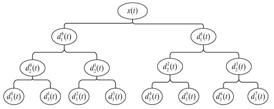
Figure 1.
Wavelet packet decomposition (WPT) decomposition process.
The represents the level of the WP tree, and represents the index of the -th node. The recursive decomposition is repeated until the maximum number of decomposition layers produces mutually orthogonal subspaces.
The wavelet packet coefficients obtained by WPT decomposition correspond to a specific subspace within the frequency resolution range of the same decomposition scale, which contains the node signal information corresponding to different frequency bands. The formula of the node coefficients at different decomposition scales of the WP tree structure is as follows.
where denotes the wavelet packet coefficient corresponding to the -th node in the th layer. and denote the decomposition scale of the WP tree and the node index at the corresponding scale. The wavelet packet coefficient can better characterize the fault information corresponding to different frequency bands. Energy is an important indicator to measure how much information a specific WPT node contains. It contains a large amount of fault information that is easy to distinguish. The energy fluctuation in a specific component corresponds to the specific fault. Next, we will construct an energy spectrum matrix based on the wavelet packet coefficients to realize the initial feature expression of the original vibration signal.
2.2. Construction of Wavelet Packet Energy Spectrum Matrix
Using WPT decomposition theory, we decompose the original vibration signal into layers and obtain mutually orthogonal subspaces. In the process of constructing the energy spectrum matrix, WPT is a key stage of data preprocessing, and the influence of WPT decomposition layers on model performance and classification accuracy should be studied. A small number of decomposition layers cannot well reflect the energy flow pattern in the original vibration signal, the fault information contained is simpler and the robustness is poor. The large number of decomposition layers will lead to complex calculations and also contain some redundant energy information. After comprehensive consideration, we use 8-layer WPT for decomposition.
In the experiment, we selected 1024 sampling points as a group of rotating machinery failure experiment samples. Using WPT to decompose the original vibration signal in eight layers, a total of frequency band subspaces are obtained. Each frequency band subspace corresponds to four wavelet packet coefficients; . represents the number of layers of wavelet packet decomposition. Since the wavelet packet coefficient can better characterize the fault information of each frequency band subspace, the frequency band energy value corresponding to each node can be calculated by the wavelet packet coefficient, thereby measuring the fault information contained in a specific WPT node. The energy value of the frequency band corresponding to the node in each subspace can be calculated by the wavelet packet coefficient, as shown in the following formula.
where represents the energy value calculated by the -th node in the -th layer according to the wavelet packet coefficients. represents the wavelet packet coefficient of the -th node in the -th layer. can be calculated by Equation (3) above. represents the sub-energy value contained in each wavelet packet coefficient in each frequency band subspace. The total energy value of each frequency band subspace is the sum of squares of all wavelet packet coefficients in the space. represents the number of wavelet packet coefficients corresponding to each subspace. In order to normalize the energy of each frequency band, the percentage of energy of each component (normalized energy value) is defined as follows.
represents the sum of the frequency band energy corresponding to all frequency band subspaces of layer . The energy values of the frequency bands corresponding to all the nodes of the -th layer can be obtained from Equation (5), and the following energy vectors are constructed for the energy of the nodes from the low frequency to the high frequency of the -th layer.
In this paper, a total of frequency band subspaces are obtained by WPT decomposition for each sample, so the energy vector dimension obtained is 256, which corresponds to the energy value of each frequency band subspace after WPT decomposition. The input data are converted to 256 dimensions by the energy spectrum matrix from 1024 sampling points, which realizes the initial dimension reduction in the input data.
Convert the energy feature vector into a new two-dimensional matrix space and reconstruct the dynamic structure of the spectrum distribution. In this process, for the convolutional neural network, the convolution kernel function can deeply monitor the spectrum energy fluctuations and local relationships, which is conducive to extract invariant but accurate details of robust features. The energy spectrum matrix is constructed as follows.
This two-dimensional energy spectrum distribution space demonstrates the energy flow of the time–frequency subspace between different frequency bands. Each node can be regarded as a container, and the failure mode change in the non-stationary time–frequency distribution will form a unique energy flow in the container. For different failure modes of rotating machinery, the internal non-stationary changes and failure information will be revealed in the energy spectrum matrix, so the energy spectrum matrix can be used as the characteristic expression form of the subsequent input model.
3. Adaptive Hierarchical Fault Diagnosis Model (A-HDCNN)
In this part, we propose a new two-stage hierarchical fault diagnosis model (A-HDCNN, adaptive hierarchical deep convolutional network). In view of the characteristics of the traditional two-dimensional convolutional model at this stage, the inherent learning rate causes slow convergence and low diagnostic performance. From the model training method, this paper further proposes an adaptive learning rate dynamic adjustment strategy, which overcomes the traditional limitations of inherent learning rate. This strategy improves model training speed and diagnostic accuracy and prevents vanishing gradient problems associated with most deep learning methods. The task of the A-HDCNN model proposed in this paper is not just accurate fault location classification, the hierarchical structure of A-HDCNN can further judge the severity level. The A-HDCNN model meets the needs of current fault diagnosis. The model is composed of two parts: the failure mode determination layer and the failure severity evaluation layer. The following sections will be described in detail.
3.1. Overview of Combination Mechanism of Energy Spectrum Matrix and A-HDCNN
Convolutional neural network (CNN) is a typical deep feedforward network [31]. On the whole, CNN is mainly divided into two stages: feature extraction and classification. The feature extraction stage is mainly composed of multiple convolutional layers and pooling layers alternately connected. After the feature learning is completed, it enters the classification stage. The feature map after feature learning is reconstructed and imported into a fully connected network for classification. The output of the network is generally a Softmax layer, which is used to calculate the probability output of the multi-classification problem.
The convolutional layer has the characteristics of weight sharing and local connection, and features are extracted through the convolution kernel. The convolution operation is defined as follows.
where is a set of input feature maps and represents the -th input feature map of the . layer. represents the convolution kernel connecting the -th input feature map and the -th feature map, which is composed of a weight matrix. corresponds to the offset term of the current convolution operation. represents convolution operation and corresponds to the non-linear activation function of the current convolution layer.
It is difficult to achieve continuous recognition of failure modes and failure severity at the same time. It is necessary to extract highly representative features and powerful intelligent fault diagnosis models. The effective combination of the energy spectrum matrix and the adaptive hierarchical convolutional neural network A-HDCNN meets this requirement. As WPT has the characteristics of multi-resolution, it overcomes the shortcomings of poor resolution of wavelet decomposition in high frequency bands. This paper uses WPT to perform multi-scale decomposition to extract multi-scale spatial energy features to construct an energy spectrum vector. It is transformed into a two-dimensional energy spectrum matrix and reconstructed dynamic structure of energy distribution. Compared with the original vibration signal, the dimensionality of the input data is greatly reduced. The energy spectrum matrix removes part of the redundant features and fully characterizes the fault information of the original vibration signal. For the hierarchical diagnosis network proposed in this paper, it is more necessary to obtain a simplified model with fast adjustment speed and high robust performance. The highly representative features of the energy spectrum matrix provide conditions for the adaptive extraction of robust features from the A-HDCNN model. In this process, for the convolutional neural network, the convolution kernel function can deeply monitor the spectral energy fluctuations and local relationships. It is beneficial to extract robust features that are invariant but precise in detail. Compared with other deep learning models, convolutional neural networks have the characteristics of weight sharing and local connection. The complexity of the model parameters is greatly reduced, which further lays the foundation for the subsequent improvement of model diagnosis accuracy and convergence speed. Therefore, the effective combination of the energy spectrum matrix and the A-HDCNN model further ensures the performance advantages of rotating machinery fault diagnosis. Subsequent experimental verification will further prove this conclusion.
3.2. Construction Process of Two-Level Hierarchical Network
In the next experiment, we used the case data set of Case Western Reserve University as an example to explain the composition process of the A-HDCNN model. It includes health status and three types of faults, namely, inner fault (IF), outer fault (OF), rolling fault (RF), and each fault type has three severity levels. This paper has designed two corresponding functional layers (L1 and L2), which are used for failure mode determination and failure severity evaluation, respectively. The composition of the two-level hierarchical network structure is shown in Figure 2.
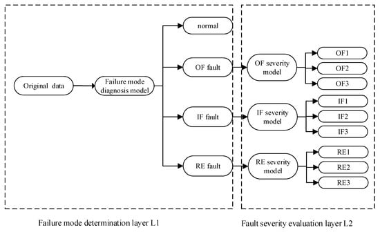
Figure 2.
Adaptive hierarchical deep convolutional network (A-HDCNN) model architecture proposed in this paper.
3.3. Failure Mode Determination Layer
The A-HDCNN hierarchical model provides an efficient method for automatically extracting features from a series of signals and can accelerate the convergence of the model and improve the diagnostic performance of the model. The first layer is the failure mode determination layer. Assuming that the bearing failure mode has a C-type failure, we define the class labels as , and construct a data set with the number of samples N based on the proposed energy spectrum matrix. represents the input vibration signal vector, represents the corresponding sample label. Then the training samples are put into the first layer network for failure mode determination. The first layer of the A-HDCNN model is based on the classic LeNet5 convolution model. The proposed sub-model structure of A-HDCNN is shown in Figure 3. Each plane is a feature map with a set of weight units that must be determined.
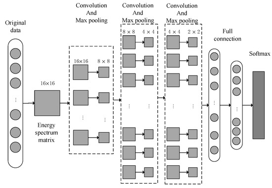
Figure 3.
Sub-model structure corresponding A-HDCNN.
The first layer structure of A-HDCNN is used for failure mode determination. There are seven main layers. The first layer pre-processes the original vibration signal and uses WPT decomposition to construct the energy spectrum matrix as the model input. This is a typical deep convolution model input form. The next three layers are convolutional and pooling layers, and each layer contains a convolutional layer and a maximum pooling layer. The number of convolution kernels in the first, second, and third convolutional layers is 8, 16, and 16, respectively, and the corresponding pooling matrix size is uniformly set to 2 × 2. In order to extract more streamlined features for classification, we set up two fully connected layers. In the last layer of the convolution and pooling layer, we reconstruct the last feature map obtained as vector input for the fully connected layer. The last layer is the logistic regression layer and uses the Softmax method for classification. The weights of each layer are randomly initialized and optimized for training. We use the Adma optimizer for parameter optimization training. After the training is completed, the test samples are input to the model for accuracy and performance evaluation. The detailed parameters of the specific A-HDCNN sub-model structure are shown in Table 1.

Table 1.
A-HDCNN sub-model structure detailed parameter description.
Figure 4 shows the A-HDCNN sub-model training process based on this method. The process is mainly composed of three parts: data preprocessing, network training and network testing—summarized as follows.
- The acceleration sensor is used to obtain the original vibration signal of the rotating machinery and construct a sample set. For each set of samples , is the observation sequence of the original vibration signal, and is the actual fault label of . is the total number of fault categories.
- Perform data preprocessing on each set of sample observation sequence to obtain the corresponding feature sample set , where is the feature mapping of the sample observation sequence in the time–frequency space. First, use WPT to decompose the observation sequence . in layers, and obtain the frequency band subspac from low frequency to high frequency. For each subspace , calculate the energy corresponding to each subspace according to the wavelet packet coefficient, and construct an energy spectrum vector, . Normalize and convert it to a two-dimensional energy spectrum matrix to obtain .
- Combine the feature sample sets of different fault categories and split them into training set, validation set and test set.
- Construct hierarchical convolutional neural network models, which are N sub-models, respectively, including one failure mode determination layer and (N − 1) failure severity evaluation layer. Initialize model parameters, number of iterations and training batches. The detailed description of specific model parameters is shown in the Table 1.
- Train each sub-model and use cross entropy as the loss function of the training model parameters. For the feature set samples corresponding to each training batch, the cross-entropy function is used to calculate the model error loss, and the gradient descent algorithm is used to update the parameters of each layer of the model until the model converges to the minimum value, which indicates that the model training is completed.
- Repeat step 5 until all N sub-models in the hierarchical model are trained.
- The test set was used to verify the diagnostic performance of the model. In order to obtain stable results, 20 tests were performed, and the average accuracy rate was obtained.

Figure 4.
A-HDCNN sub-model training process.
Figure 4.
A-HDCNN sub-model training process.

3.4. Fault Severity Evaluation Layer
Taking the CWRU bearing data set as an example, after determining the failure mode through the first layer model, the corresponding normal, inner, outer, and rolling bearing health status are obtained. For the three failure modes, we continue to establish a corresponding evaluation model in the second layer to evaluate its failure severity level. Each evaluation model has the same structure as the first layer of A-HDCNN, because the related samples have the same size of fault damage. As mentioned above, the weights of each layer are randomly initialized and optimized for training. However, after training, the test sample is input into the evaluation model, and the output is a probability vector. The corresponding sample has been evaluated by the model to obtain a larger size probability value, indicating that the sample is more likely to be of such severity. Due to the need for size identification, there will be other situations with different severity in the actual operating environment, so we propose a method to calculate the failure size of each sample instead of providing a simple label. Enter the test samples into the model, and the probability that each sample belongs to each fault severity level is as follows.
The fault damage size of each sample is a mapping of its model predicted probability value, which can be calculated as follows.
where is the failure severity level of the -th category, is the failure damage level corresponding to a certain failure mode, and is the probability that the -th failure sample belongs to the -th severity level, which enables the system to output the predicted result of the fault severity.
3.5. Adaptive Learning Rate Dynamic Adjustment Strategy
After establishing the failure mode determination layer and the failure severity recognition layer, the next step is to train the model and update the weight parameter to minimize the target loss function. Since cross entropy can speed up the update of weights and the convergence of the entire model, this paper uses the cross-entropy loss function, which is defined as follows.
where represents the total number of categories, represents the true label of the sample predicted as the -th category, and represents the actual probability output of the sample predicted as the -th category. We use back-propagation rules and supervised training methods. First, use the cross-entropy loss function to calculate the error loss of the Softmax layer output, and then calculate the gradient corresponding to the convolution kernel parameter of each layer of the model through the back-propagation algorithm, and update the model weight parameter to obtain a smaller output error. Suppose and are the input samples and output vectors of the model, and is the output label of . Therefore, the corresponding output error is defined as follows.
is the loss function, and is the weight or offset that needs to be updated for each convolution kernel. The update strategy is as follows.
represents the learning rate during training. A proper learning rate ensures the convergence speed and accurate performance of model training.
In the traditional model training method, the learning rate is usually set to a fixed value, and the optimal value is often obtained based on experience. A larger or smaller value will have an adverse effect on model training. Generally speaking, a larger learning rate will cause the model loss error to oscillate, and a smaller learning rate will result in poor model convergence performance, so it is difficult to balance.
Due to the difference in model feature learning situation and loss error convergence in different iterative training processes, and for the fixed learning rate, in the early, middle and late stages of training, if a certain learning rate for the initial stage is better for the model performance, other stages may have adverse effects. Therefore, in the research process of this paper, a learning rate adaptive update strategy is proposed, which will dynamically adjust the learning rate in real time in stages according to different iterative processes in training. The learning rate adaptive update formula is as follows.
where and are the learning rate of the -th iteration and () iteration of the model training, respectively. and are the value of the loss function for the th iteration and the () iteration. In the early stage of the iteration, in order to accelerate convergence, the learning speed is increased according to the relative change of the error loss. The learning rate changes within a relatively fast range. At the later stage of the iteration, the relative change of the error loss is small, so the learning rate gradually slows down and tend to be stable. Assuming , it means that the model is in the oscillation stage, and the learning rate will decrease with the degree of oscillation during the adjustment process. Assuming , the model error loss is in the normal decay process, and the learning rate adaptively and dynamically changes according to degree of the error decay. The learning rate update rule corresponding to the method proposed in this paper shows this training process. According to the adaptive adjustment strategy of dynamic learning rate, the update rules of weight and offset corresponding to each convolution layer and fully connected layer of the specific model are as follows.
4. Experimental Verification
4.1. Experimental Data Description
In order to verify the effectiveness of the proposed method, experiments were carried out on the defective bearing data set of the CWRU Bearing Data Center. The main components of the experimental device used for the experiment include a 2 hp motor, a power meter, a torque sensor and an electronic control device, as shown in Figure 5. The bearing model is SKF6205, the roller diameter is 7.5 mm, the cross-sectional diameter is 39 mm, the number of rollers is 9, and the contact angle is 0°. This bearing is machined by electrical discharge (EDM). There are three types of defects in EDM. The single-point faults with dimensions of 0.007, 0.014 and 0.021 inches are installed on the outer ring (OR) and inner ring (IR) of the test bearing, and on the rolling element (RE). The vibration data are collected by an accelerometer with a sampling frequency of 12 kHz. In short, a healthy state and three defect states (each with three severe injury levels) constitute the experimental verification data set. For each failure type, 50 samples are randomly selected for training, and another 50 samples are randomly selected for testing. Table 2 provides a detailed description of the experimental data set. The typical waveforms of 10 health states are shown in Figure 6. It can be seen that the time-domain waveform can initially indicate the pulses related to the fault, but in some cases, there will be greater noise. Figure 7 shows the FFT spectrum corresponding to the 10 original healthy vibration signals. In the FFT spectrum, the characteristic frequency also submerged in noise. In addition, both the time-domain waveform and the FFT spectrum lack non-stationary information. Based on the FFT spectrum, we select the amplitude of the random variable in the spectrogram as a benchmark and make a probability distribution histogram for observation. Figure 8 shows the probability distributions corresponding to the original vibration signal spectra under 10 health states. Compared with the FFT spectrum, the probability distributions of different health states are somewhat different, but due to noise interference, the distinction is not obvious.
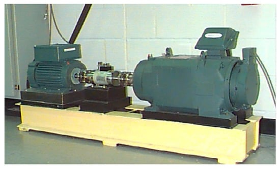
Figure 5.
Experimental device for obtaining vibration signals of rolling bearings.
Table 2.
Experimental data and parameter description.
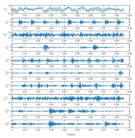
Figure 6.
Raw signal of rolling bearing vibration under different failure modes.
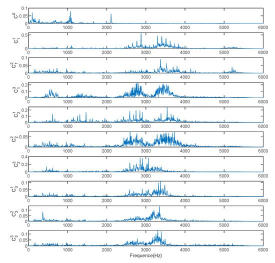
Figure 7.
Fast Fourier transform (FFT) spectrum corresponding to the original vibration signals of 10 health states.
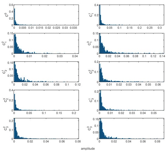
Figure 8.
Histogram of probability distribution of FFT spectrum based on 10 health states.
In order to verify the robust performance of the proposed model under different load environments, four experimental data sets (A–D) are set in this paper for verification, as shown in Table 3.
Table 3.
Introduction of experimental data sets under different load environments.
4.2. Analysis of Experimental Results of WPT Energy Spectrum Matrix Construction
The features contained in the WPT energy spectrum matrix proposed in this paper can provide correct fault information for fault diagnosis. Using WPT to decompose the original vibration signal in 8 layers, the branch signals corresponding to frequency band subspaces are obtained. To facilitate observation, we take the signals corresponding to the first 8 nodes for observation. As shown in Figure 9, the bearing vibration signal WPT in the healthy state under the 1hp load environment decomposes the first eight branch signals corresponding to low frequency to high frequency. The energy value of the frequency band is calculated for each branch signal, and the WPT energy spectrum vector calculated by the vibration signals corresponding to the 10 fault types is shown in Figure 10. As the input of the model, we reconstruct it and convert it to . energy spectrum matrix. We found that for different failure modes, the energy spectrum vectors show a strong difference. Compared with the original vibration signal FFT spectrum, the expression is enhanced. Therefore, the energy spectrum matrix as a raw vibration signal data preprocessing has a strong applicability. At the same time, it is used as the input of the A-HDCNN model, which reduces the input data dimension and model complexity, and improves the ability to express features. It can be observed that different fault conditions exhibit different frequency band energy characteristics and show strong differences. Therefore, the energy spectrum matrix constructed by WPT decomposition can be used as a characteristic form of subsequent failure mode diagnosis.
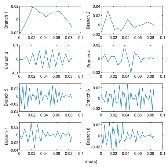
Figure 9.
WPT decomposition branch signal of normal bearing vibration signal.
Figure 10.
WPT energy spectrum vector under different health states of bearings.
4.3. A-HDCNN Model Diagnosis Results
In order to verify the superiority of the proposed A-HDCNN model, at the same time, the performance difference between HDCNN and A-HDCNN model after learning rate adaptive dynamic adjustment law is compared. We use the bearing data set of CWRU for experiments. The energy spectrum matrix obtained by preprocessing the original vibration signal is used for the input of the model. Through training, the weight parameters of the model are adjusted, and the performance of the trained model is tested with test samples. During the sample construction process, we collected data under different motor load environments. Under each load, 100 sets of samples were collected for each of the 10 health states, of which 50 sets were used for training and 50 sets were used for testing. A total of 1000 sets of samples were collected under the same load. All the samples in the healthy state are used in the first layer failure mode determination layer, and a total of 1000 samples are used for training (500 samples) and testing (500 samples). In the second layer of fault severity evaluation layer, there are three types of fault severity for each fault mode. Use 150 samples for training and 150 samples for failure severity assessment. The initialization parameter configuration for the specific training of each layer model is shown in Table 4.
Table 4.
Model initialization parameter configuration.
The learning rate is the coefficient of the gradient in the stochastic gradient descent (SGD) process, and it is directly related to the performance of model parameter optimization. Too high a learning rate will hinder optimization and cause loss errors to oscillate, while a too low learning rate will result in poor model convergence performance and fall into a local optimum. In traditional model training methods, the learning rate is usually set to a fixed value, and a larger or smaller value will adversely affect the model training. Many researchers choose the learning rate based on experience. For the A-HDCNN model proposed in this paper, the adaptive learning rate dynamic adjustment strategy realizes the dynamic matching of the dynamic adjustment of the learning rate and the number of iterations during the training process. The corresponding learning rate is always guaranteed to be updated along the direction of the gradient and has an appropriate learning rate. The initial learning rate of the model has almost no effect on the convergence of the final A-HDCNN model. In order to conduct comparative experiments, for the HDCNN model, it is still a fixed learning rate adjustment. We select fixed learning rates at equal intervals for experiments to observe the convergence and accuracy changes of different learning rate settings for different sub-models. The experiment found that the model is optimal and has a high accuracy and convergence performance when the learning rates of the first layer of failure mode determination layer and the second layer of fault severity evaluation layer , , were set, respectively, at 0.0035, 0.0040, 0.0040, 0.0075. In order to reduce the influence of other experiments, the initial value of the learning rate of the A-HDCNN model is set to be consistent with HDCNN.
Since each model corresponds to a large number of training samples, the samples are randomly split and combined. A small batch of samples is used to pack and input to the A-HDCNN model for training, and then the parameters are optimized according to the average error loss of each batch. "Batch size" represents the number of samples in the batch, which has a significant impact on the optimization performance and training rate of the model. For the model, the training data set and the test data set each contain 500 samples, and the batch size should be a divisor of 500, such as 100, 50, 10, 5, 1, otherwise it will cause sample waste. For the , , , the training data set and the test data set each contain 150 samples. The batch size should be a divisor of 150, such as 30, 10, 5, 1. If the batch is small, the number of samples combined in each training is small, resulting in slow parameter optimization. If the batch size is large, the model will fall into the local optimum. Therefore, compare the batch size and observe the impact of different batches on the diagnosis accuracy and convergence performance. It is found that for the failure mode determination layer and the failure severity evaluation layer, the batch setting is set to 10, which has the best convergence and the highest accuracy.
The following figure shows the training and test results of the sub-models in the failure mode determination layer and the failure severity evaluation layer after adding the learning rate dynamic adjustment law under a 1hp load environment. Figure 11a shows the failure mode determination layer model dynamic adjustment curve of learning rate. It can be seen that the learning rate is dynamically adjusted in stages in real time according to different iterations in the training process. In the early stage of the iteration, in order to accelerate convergence, the learning rate in the initial stage is generally large due to the relatively large change in the loss function. Later in the iteration, the relative change of the loss function is small, so the learning rate is generally small. On the whole, due to the good feature expression ability of the energy spectrum matrix, there is less tendency to oscillate throughout the training process. The learning rate gradually decreases and converges with the number of iterations. The learning rate update rule proposed in this paper reflects this training process. Take the failure mode determination layer as an example, as shown in Figure 12a. Compared with the fixed learning rate model, after the learning rate adaptive update rule is added, the accuracy rate converges faster with the number of iterations, and convergence can be achieved around 20 generations, while the fixed learning rate can only reach convergence around 60 generations. As shown in Figure 13a, taking the failure mode determination layer as an example, the same conclusion can be drawn from the variation of error loss. In addition, for the fault severity evaluation layer, as shown in Figure 13b–d, it shows the variation curve of the error loss of the sub-model corresponding to the fault severity evaluation layer with the number of iterations. After adding the learning rate adaptive update rule, the convergence performance is also better. Therefore, the model feature learning speed is accelerated after the learning rate update rule is added, and the same layer of feature expression ability and convergence performance within its sub-model are greatly improved. This change process verifies the reliability of the proposed method. Figure 11b–d show that the learning rate update of the fault severity assessment layer changes with the number of iterations. Figure 12b–d show the comparison of the accuracy rate change rule with the number of iterations compared with the fixed learning rate model. It can be concluded that for the sub-model of the fault severity assessment layer, update rules can have a significant performance improvement, accelerate the model convergence speed, improve the model diagnosis accuracy, and reduce the model loss error. These results verify the performance advantages of the A-HDCNN model in fault diagnosis.
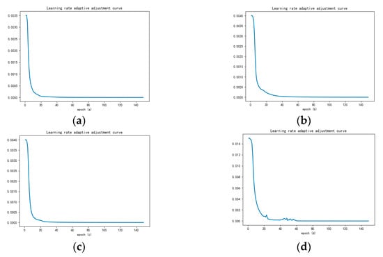
Figure 11.
Model learning rate adjustment law: (a) Model; (b) Model; (c) Model; (d) Model.
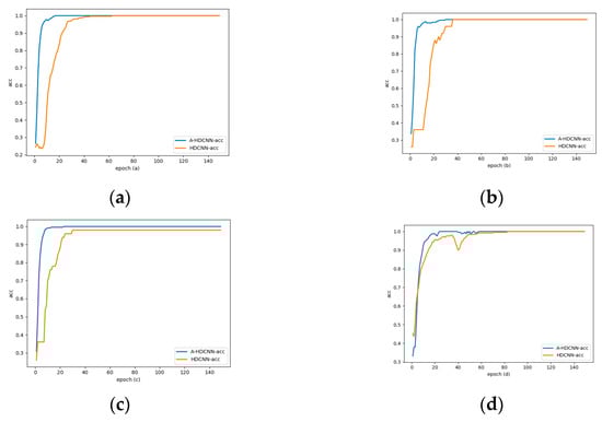
Figure 12.
Accuracy rate change curve: (a) and accuracy rate change curve; (b) change in accuracy of and ; (c) change in accuracy of and ; (d) change in accuracy of and .
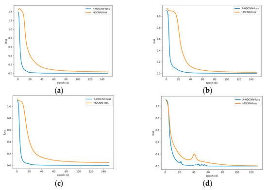
Figure 13.
Error loss changes with the number of iterations: (a) Model; (b) Model; (c) Model; (d) Model.
In order to obtain more accurate evaluation results and verify the stability of the model at the same time, the samples collected at different levels of the model are randomly split and shuffled, and the training set and test set are reconstructed. We conduct 20 random selection verifications. As shown in Table 5, the average diagnostic accuracy of different algorithms under different load environments during 20 runs is summarized. Through observation, it is found that the A-HDCNN model has higher recognition accuracy at the first layer. The diagnostic accuracy is 100%, and they can all be correctly classified. At the same time, it indicates that the failure modes can be correctly flowed into the corresponding severity evaluation layer. The second layer sub-model did not accept incorrect failure mode samples. This good performance laid a good evaluation foundation for subsequent failure severity evaluation, and also verified the superiority of the energy spectrum matrix in the determination of failure mode. The features are easy to distinguish, and the learning ability of the model is good.
Table 5.
Comparison of model diagnosis accuracy between A-HDCNN and HDCNN under different load environments.
At the second level, we evaluate the severity of the failure. Table 5 shows the comparison of the accuracy of the failure severity assessment for each health condition under different load environments. The classification results show that the evaluation of the A-HDCNN model at the second layer has high accuracy, and the diagnostic accuracy is as high as 99% or more, close to 100%. The diagnostic accuracy is stable under different loads. In addition, it shows that the overall model has high diagnostic accuracy as shown in Table 5.
In addition, in order to further measure the variable load capacity of the A-HDCNN model and verify its adaptability under different load environments, we combined and shuffled the B, C, and D data sets (1hp, 2hp, and 3hp load environments, respectively), and constructed a training set and a test set. Train the model and test the experimental results, as shown in Table 5. It can be found that the A-HDCNN model has high diagnostic accuracy in both failure mode recognition and fault severity evaluation, close to 100%, which further proves the robustness of the A-HDCNN model under variable load environment.
Error loss is an important indicator of model stability. In order to verify the influence of adding learning rate adaptive adjustment strategy on model stability, we summarized the average error loss of different algorithms under different load environments during 20 runs (iteration 150 times), as shown in Table 6. It can be concluded that whether it is the failure mode determination layer or the failure severity evaluation layer, the A-HDCNN model is more stable under various load environments, and the error loss can converge to a minimum. Compared with the HDCNN model, the A-HDCNN model has a smaller error loss. In addition, after verification of the B, C, and D mixed data sets, the A-HDCNN model error can still converge well and the loss is small, which further verifies the stability and robustness of the A-HDCNN model in a variable load environment.
Table 6.
Comparison of model error loss between A-HDCNN and HDCNN under different load environments.
In order to further verify the reliability of the A-HDCNN model, and to verify the performance advantages of the combination of the energy spectrum matrix and the A-HDCNN model, we compare the performance of the typical algorithms commonly used at this stage, namely, DNN and SVM. In addition, in order to reflect the effectiveness of the proposed method, we replace the A-HDCNN model with DNN or SVM in the same hierarchical structure. The two algorithm inputs are energy spectrum vectors to achieve similar layer recognition. DNN uses the ReLU function as the activation function. In SVM, we choose the radial basis function for classification. Table 7 shows the specific diagnosis results. Through observation, it is found that, compared with the deep fully connected neural networks DNN and SVM, the A-HDCNN model can achieve higher accuracy in both failure mode determination and failure severity evaluation. The overall model diagnostic accuracy is as high as 99.74%, which is better than DNN and SVM. At the same time, for the evaluation of fault severity, the characteristics of samples with different severity under the same fault mode are difficult to distinguish and confuse, which makes the diagnosis and learning of DNN and SVM difficult. In addition, for DNN and SVM models, the problem of poor diagnostic accuracy of the first layer further makes the second layer model receive samples of wrong failure modes, which further reduces the diagnostic accuracy of the second layer model. At the same time, it is also proved that the A-HDCNN model can adaptively extract the robust characteristics of the energy spectrum matrix with constant and precise details, which further proves the combined advantages of the energy spectrum matrix and the A-HDCNN model.
Table 7.
A-HDCNN model diagnostic accuracy of each layer compared with existing methods.
The A-HDCNN model provides a systematic and complete method for bearing fault diagnosis and overcomes the limitations of traditional training methods that use a fixed learning rate on model diagnostic performance. The adaptive learning rate dynamic adjustment strategy ensures that the model can adaptively extract robust features. It is highly adaptable under different load environments and has better diagnostic performance. In order to verify the superior performance of the adaptive method proposed in this paper, we use the overall diagnostic performance of the model as an indicator to compare the overall performance of the A-HDCNN model with other superior adaptive methods proposed by researchers in the field of fault diagnosis at this stage. For example, in order to improve the efficiency of continuous learning elements of rolling bearing fault diagnosis, Tian et al. [32] incorporated a clonal learning strategy into the convolutional network (DCNN-FD-Softmax), which can adaptively extract deep fault features. Xie et al. [33] proposed an end-to-end fault diagnosis model based on an adaptive deep belief network (Improved DBN+FFT). Qiao et al. [34] proposed an adaptive weighted multi-scale convolutional neural network (AWMSCNN) for bearing diagnosis under variable operating conditions. At the same time, we use the energy spectrum matrix and deep convolutional neural network method under the single-level model as a benchmark for reference. The comparison results are shown in Table 8. The experimental results show that the proposed method performs higher than other adaptive methods. The test accuracy is 99.74%, which is mainly the result of the better feature expression of the energy spectrum matrix and the adaptive feature learning ability of the A-HDCNN model. The experimental results are satisfactory. The comparison results show that compared with other methods, the A-HDCNN model proposed in this paper has achieved significant results and is better than other adaptive methods. It can be seen that the A-HDCNN model proposed in this paper has significant performance.
Table 8.
Comparison of the overall performance of the A-HDCNN model with other adaptive diagnosis methods.
4.4. Feature Visual Verification with T-SNE
The neural network can automatically learn features from vibration signals. This article explores the internal operation process of the proposed A-HDCNN model by visualizing the activities in the neural network, and further verifies the adaptive feature learning ability of the proposed A-HDCNN model. As the internal structure of the first-level model and the second-level model is similar, they have the same internal mechanism. This paper analyzes the fault pattern recognition layer and uses t-SNE to visualize the learning characteristics of the model input layer, an intermediate convolution layer, and a fully connected layer.
Taking data set B as an example, the experimental results are shown in Figure 14. The model input layer is the energy spectrum matrix obtained by preprocessing the original vibration signal. Compared with the chaotic distribution of the original signal, the different health states of the input layer of the model are easier to segment. It is found that the samples of the same failure mode can basically be gathered together. The normal state samples have good aggregation and the sample spacing is large, but there is some overlap in the IR, OR, and RE failure mode. The distance between the classes is small, and the feature recognition of the input layer and the intermediate convolutional layer is poor. However, as the depth of the layer increases, the features learned by the convolutional layer become more and more recognizable and the features become more and more divisible. In the early layer, it cannot be divided, but in the fully connected layer, the characteristics are very easy to be divided. As shown in Figure 14c, the four failure modes are effectively distinguished, and their characteristics are almost no overlap of different failure types. The distance between different categories is large. It is proved that the model can adaptively learn effective features and perform accurate fault diagnosis.
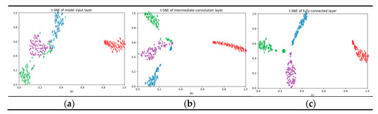
Figure 14.
T-SNE visualization: (a) the model input layer; (b) the intermediate convolutional layer; (c) the fully connected layer.
4.5. Robust Performance Analysis of A-HDCNN Model under Different SNR Environments
The stability and robustness of the A-HDCNN model are very important evaluation indicators in practical engineering applications. CWRU bearing data are collected under different health conditions and different working conditions, and its original vibration signal already contains a certain degree of noise. In order to better simulate the strong noise interference in the actual operation process, we added corresponding Gaussian noise under different signal-to-noise ratios (SNRs) to the original vibration signal to further verify the stability and robust performance of the proposed method. The specific definition of SNR is as follows.
where and represent the intensity of original signal and noise, respectively, we assume is 0 dBW. In this experiment, we will verify the effectiveness of the proposed A-HDCNN model in different noise environments. In order to facilitate the comparative test, we will carry out diagnostic analysis under 1hp load environment, and its SNR is between −8 db and 12 db. At the same time, the HDCNN model, WPE+DNN, WPE+SVM were used as the benchmark for comparative analysis. The experimental results are shown in Figure 15 and Table 9. Obviously, A-HDCNN is superior to the other three benchmark methods, and it can obtain the best diagnostic performance in any noisy environment. In addition, the model has a diagnostic performance of more than 94% at all noise levels, except for the diagnostic accuracy of 87.36% at −8 dB. When the SNR continues to increase, the A-HDCNN model and the HDCNN model, WPE+DNN, WPE+SVM benchmark models have the same increasing trend, and their diagnostic accuracy increases with the increase in the SNR. In addition, we can also infer that the diagnosis error is mainly due to the similarity of the fault feature itself and the difference between the models when the noise is small. That is to say, under different working environments, some different fault signal features may overlap or be close to each other, thereby affecting the accuracy of diagnosis. However, the accuracy of the A-HDCNN model is close to 100% when the noise environment is small, which means that the model has better fault feature learning ability and expression ability, and can have the ability to extract the most essential difference between various fault features. On the other hand, although the performance of all methods decreases with increasing noise, the A-HDCNN model still exhibits good noise immunity in a strong noise environment. Therefore, compared with several other benchmark methods, the A-HDCNN model has stronger anti-noise ability and fault feature learning ability under different noise environments. The A-HDCNN model has strong robustness and stability to noise and is more suitable for the diagnosis of rotating bearing faults in actual operation.
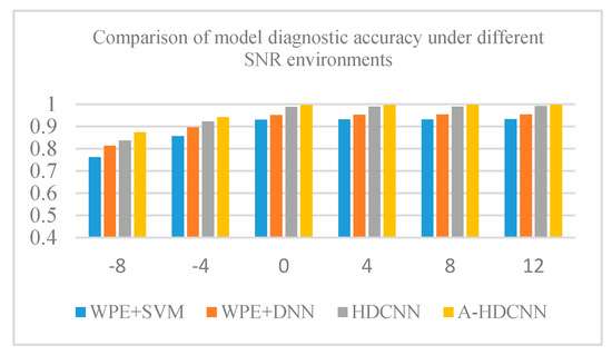
Figure 15.
Comparative analysis of overall model diagnostic performance under different SNR environments.
Table 9.
Comparison of model diagnostic accuracy under different signal-to-noise ratio (SNR) environments.
5. Conclusions
This paper proposes a new A-HDCNN network for fault diagnosis of rotating machinery bearings. The model is a two-layer hierarchical diagnostic network that can be used for both fault pattern recognition and fault severity evaluation. This method has the following characteristics.
Firstly, in view of the non-stationary characteristics of the original vibration signal of the fault, a representative energy spectrum matrix is proposed for the input of the model, while reducing the dimension of the input data. It overcomes the limitations of model parameter adjustment, model complexity increase, and slow convergence caused by direct input of the original vibration signal into the model. Compared with the traditional feature selection method, this kind of data preprocessing method greatly reduces the experience of experts. It can be observed through the diagnosis results under different load environments at a later stage. This method has good robust performance and high applicability under different load environments.
In addition, the hierarchical structure of A-HDCNN makes the model parameters of each layer relatively independent and individually adjusted, thereby further ensuring the efficiency of diagnosis, which can assess the location of the fault and the severity of the fault. In this way, weak links can be discovered, thereby preventing system degradation and providing knowledge for reliability design and life prediction of rotating machinery.
Secondly, the traditional model training method often uses a fixed learning rate to update the parameters. Larger or smaller values will adversely affect the model training, so it is difficult to balance. Due to the differences in model feature learning conditions and loss error convergence in different iterative training processes, this paper proposes an adaptive update strategy for learning rate during the research process, so that the learning rate is adaptively and dynamically adjusted at different stages of model training. It is applied to the training process of the sub-model of the failure mode determination layer and the severity evaluation layer. Compared with the traditional HDCNN model and other hierarchical methods, it further verifies the feature learning ability, convergence and reliability of the method.
Finally, in order to further verify the robustness and stability of the model and better simulate the strong noise interference during actual operation, the corresponding Gaussian noise under different SNRs is added to the original vibration signal. By comparing other methods such as HDCNN, WPE+DNN, and WPE+SVM, it further proves the effectiveness of the A-HDCNN model in different noise environments and is more suitable for fault diagnosis of rotating bearings in actual operation.
Author Contributions
Y.L. finalized the version to be published; Y.Y. conceived and designed the topic and wrote the paper; T.F., Y.S. and X.Z. refined the idea and revised the paper. All authors have read and agreed to the published version of the manuscript.
Funding
This work was supported in part by the Revitalizing Liaoning Outstanding Talents Project under Grant XLYC1907057, in part by the National Nature Science Foundation of China under Grant U1908212, in part by the Key Project of Natural Science Foundation of China under Grant 61533015, in part by the National Key R&D Program of China under Grant 2018YFB1700200.
Institutional Review Board Statement
Not applicable.
Informed Consent Statement
Not applicable.
Data Availability Statement
The data provided by this study is available on Bearing Data Center Official Website of Case Western Reserve University. https://csegroups.case.edu/bearingdatacenter/home.
Conflicts of Interest
The authors declare no conflict of interest.
References
- Cao, H.; Fan, F.; Zhou, K.; He, Z. Wheel-bearing fault diagnosis of trains using empirical wavelet transform. Measurement 2016, 82, 439–449. [Google Scholar] [CrossRef]
- Wang, Z.; Zhang, Q.; Xiong, J.; Xiao, M.; Sun, G.; He, J. Fault Diagnosis of a rolling bearing using wavelet packet Denoising and random forests. IEEE Sens. J. 2017, 17, 5581–5588. [Google Scholar] [CrossRef]
- Tian, J.; Morillo, C.; Azarian, M.H.; Pecht, M. motor bearing fault detection using spectral kurtosis-based feature extraction coupled with k-nearest neighbor distance analysis. IEEE Trans. Ind. Electron. 2016, 63, 1793–1803. [Google Scholar] [CrossRef]
- Wang, S.; Chen, X.; Tong, C.; Zhao, Z. Matching Synchrosqueezing wavelet transform and application to Aeroengine vibration monitoring. IEEE Trans. Instrum. Meas. 2017, 66, 360–372. [Google Scholar] [CrossRef]
- Liu, J.; Li, Y.; Zio, E. A SVM framework for fault detection of the braking system in a high speed train. Mech. Syst. Signal Process. 2017, 87, 401–409. [Google Scholar] [CrossRef]
- Meng, Z.; Guo, X.; Pan, Z.; Sun, D.; Liu, S. Data segmentation and augmentation methods based on raw data using deep neural networks approach for rotating machinery fault diagnosis. IEEE Access 2019, 7, 79510–79522. [Google Scholar] [CrossRef]
- Fu, Q.; Jing, B.; He, P.; Si, S.; Wang, Y. Fault feature selection and diagnosis of rolling bearings based on eemd and optimized elman_adaboost algorithm. IEEE Sens. J. 2018, 18, 5024–5034. [Google Scholar] [CrossRef]
- Hu, Q.; Qin, A.; Zhang, Q.; He, J.; Sun, G. Fault diagnosis based on weighted extreme learning machine with wavelet packet decomposition and KPCA. IEEE Sens. J. 2018, 18, 8472–8483. [Google Scholar] [CrossRef]
- Tang, S.; Yuan, S.; Zhu, Y. Deep learning-based intelligent fault diagnosis methods toward rotating machinery. IEEE Access 2020, 8, 9335–9346. [Google Scholar] [CrossRef]
- Li, Y.; Zou, L.; Jiang, L.; Zhou, X. Fault Diagnosis of Rotating Machinery Based on Combination of Deep Belief Network and One-dimensional Convolutional Neural Network. IEEE Access 2019, 7, 165710–165723. [Google Scholar] [CrossRef]
- Zhang, C.; He, Y.; Yuan, L.; Xiang, S. Analog circuit incipient fault diagnosis method using DBN based features extraction. IEEE Access 2018, 6, 23053–23064. [Google Scholar] [CrossRef]
- He, Y.; Li, C.; Wang, T.; Shi, T.; Tao, L.; Yuan, W. Incipient fault diagnosis method for IGBT drive circuit based on improved SAE. IEEE Access 2019, 7, 92410–92418. [Google Scholar] [CrossRef]
- Xia, M.; Li, T.; Xu, L.; Liu, L.; de Silva, C.W. Fault diagnosis for rotating machinery using multiple sensors and convolutional neural networks. IEEE/ASME Trans. Mechatron. 2018, 23, 101–110. [Google Scholar] [CrossRef]
- Zhang, C.; Zhang, Y.; Hu, C.; Liu, Z.; Cheng, L.; Zhou, Y. A novel intelligent fault diagnosis method based on variational mode decomposition and ensemble deep belief network. IEEE Access 2020, 8, 36293–36312. [Google Scholar] [CrossRef]
- Hu, Z.; Wang, Y.; Ge, M.; Liu, J. Data-driven fault diagnosis method based on compressed sensing and improved multiscale network. IEEE Trans. Ind. Electron. 2020, 67, 3216–3225. [Google Scholar] [CrossRef]
- Ding, X.; He, Q. Energy-fluctuated multiscale feature learning with deep convnet for intelligent spindle bearing fault diagnosis. IEEE Trans. Instrum. Meas. 2017, 66, 1926–1935. [Google Scholar] [CrossRef]
- You, W.; Shen, C.; Wang, D.; Chen, L.; Jiang, X.; Zhu, Z. An Intelligent Deep Feature Learning Method With Improved Activation Functions for Machine Fault Diagnosis. IEEE Access 2020, 8, 1975–1985. [Google Scholar] [CrossRef]
- Song, Q.; Zhao, S.; Wang, M. On the accuracy of fault diagnosis for rolling element bearings using improved DFA and multi-sensor data fusion method. Sensors 2020, 20, 6465. [Google Scholar] [CrossRef]
- Liang, T.; Lu, H. A novel method based on multi-island genetic algorithm improved variational mode decomposition and multi-features for fault diagnosis of rolling bearing. Entropy 2020, 22, 995. [Google Scholar] [CrossRef]
- Xu, G.; Liu, M.; Jiang, Z.; Söffker, D.; Shen, W. Bearing fault diagnosis method based on deep convolutional neural network and random forest ensemble learning. Sensors 2019, 19, 1088. [Google Scholar] [CrossRef]
- Yu, G.; Lin, T.; Wang, Z.; Li, Y. Time-reassigned Multisynchrosqueezing transform for bearing fault diagnosis of rotating machinery. IEEE Trans. Ind. Electron. 2021, 68, 1486–1496. [Google Scholar] [CrossRef]
- Huang, R.; Li, J.; Wang, S.; Li, G.; Li, W. A robust weight-shared capsule network for intelligent machinery fault diagnosis. IEEE Trans. Ind. Inform. 2020, 16, 6466–6475. [Google Scholar] [CrossRef]
- Ali, J.B.; Fnaiech, N.; Saidi, L.; Chebel-Morello, B.; Fnaiech, F. Application of empirical mode decomposition and artificial neural network for automatic bearing fault diagnosis based on vibration signals. Appl. Acoust. 2015, 89, 16–27. [Google Scholar] [CrossRef]
- de Jesus Romero-Troncoso, R. Multirate signal processing to improve fft-based analysis for detecting faults in induction motors. IEEE Trans. Ind. Inform. 2017, 13, 1291–1300. [Google Scholar] [CrossRef]
- Maqsood, A.; Oslebo, D.; Corzine, K.; Parsa, L.; Ma, Y. STFT cluster analysis for dc pulsed load monitoring and fault detection on naval shipboard power systems. IEEE Trans. Transp. Electrif. 2020, 6, 821–831. [Google Scholar] [CrossRef]
- Yuan, J.; Jiang, H.; Zhao, Q.; Xu, C.; Liu, H.; Tian, Y. Dual-mode noise-reconstructed EMD for weak feature extraction and fault diagnosis of rotating machinery. IEEE Access 2019, 7, 173541–173548. [Google Scholar] [CrossRef]
- Liu, Z.; Han, Z.; Zhang, Y.; Zhang, Q. Multiwavelet packet entropy and its application in transmission line fault recognition and classification. IEEE Trans. Neural Netw. Learn. Syst. 2014, 25, 2043–2052. [Google Scholar] [CrossRef]
- Wang, C.; Li, H.; Huang, G.; Ou, J. Early fault diagnosis for planetary gearbox based on adaptive parameter optimized VMD and singular kurtosis difference spectrum. IEEE Access 2019, 7, 31501–31516. [Google Scholar] [CrossRef]
- Huo, Z.; Zhang, Y.; Francq, P.; Shu, L.; Huang, J. Incipient fault diagnosis of roller bearing using optimized wavelet transform based multi-speed vibration signatures. IEEE Access 2017, 5, 19442–19456. [Google Scholar] [CrossRef]
- Xu, Y.; Zhang, K.; Ma, C.; Sheng, Z.; Shen, H. An adaptive spectrum segmentation method to optimize empirical wavelet transform for rolling bearings fault diagnosis. IEEE Access 2019, 7, 30437–30456. [Google Scholar] [CrossRef]
- Kou, L.; Qin, Y.; Zhao, X.; Chen, X. A multi-dimension end-to-end CNN model for rotating devices fault diagnosis on high-speed train bogie. IEEE Trans. Veh. Technol. 2020, 69, 2513–2524. [Google Scholar] [CrossRef]
- Tian, Y.; Liu, X. A deep adaptive learning method for rolling bearing fault diagnosis using immunity. Tsinghua Sci. Technol. 2019, 24, 750–762. [Google Scholar] [CrossRef]
- Xie, J.; Du, G.; Shen, C.; Chen, N.; Chen, L.; Zhu, Z. An end-to-end model based on improved adaptive deep belief network and its application to bearing fault diagnosis. IEEE Access 2018, 6, 63584–63596. [Google Scholar] [CrossRef]
- Qiao, H.; Wang, T.; Wang, P.; Zhang, L.; Xu, M. An adaptive weighted multiscale convolutional neural network for rotating machinery fault diagnosis under variable operating conditions. IEEE Access 2019, 7, 118954–118964. [Google Scholar] [CrossRef]


Publisher’s Note: MDPI stays neutral with regard to jurisdictional claims in published maps and institutional affiliations. |
© 2020 by the authors. Licensee MDPI, Basel, Switzerland. This article is an open access article distributed under the terms and conditions of the Creative Commons Attribution (CC BY) license (http://creativecommons.org/licenses/by/4.0/).