Article

Modeling the Spread of Epidemics Based on Cellular Automata

1
College of Chemical Engineering, Beijing University of Chemical Technology, Beijing 100029, China
2
Faculty of Chemical Engineering, Kunming University of Science and Technology, Kunming 650500, China
*
Authors to whom correspondence should be addressed.
Processes 2021, 9(1), 55; https://doi.org/10.3390/pr9010055
Submission received: 17 November 2020 / Revised: 23 December 2020 / Accepted: 23 December 2020 / Published: 29 December 2020
(This article belongs to the Special Issue Modeling, Control and Pathogenesis Process in Virus Infection)

Abstract

:
Mathematical modeling is a powerful tool to study the process of the spread of infectious diseases. Among various mathematical methods for describing the spread of infectious diseases, the cellular automaton makes it possible to explicitly simulate both the spatial and temporal evolution of epidemics with intuitive local rules. In this paper, a model is proposed and realized on a cellular automata platform, which is applied to simulate the spread of coronavirus disease 2019 (COVID-19) for different administrative districts. A simplified social community is considered with varying parameters, e.g., sex ratio, age structure, population movement, incubation and treatment period, immunity, etc. COVID-19 confirmation data from New York City and Iowa are adopted for model validation purpose. It can be observed that the disease exhibits different spread patterns in different cities, which could be well accommodated by this model. Then, scenarios under different control strategies in the next 100 days in Iowa are simulated, which could provide a valuable reference for decision makers in identifying the critical factors for future infection control in Iowa.

1. Introduction

Rapid globalization, frequent travel, and contacts between people across states can make infectious diseases spread at an incredible rate. Infectious diseases have repeatedly caused an increase in human mortality and social panic throughout history [1], and countries all over the world are struggling with coronavirus disease 2019 (COVID-19) as this paper is being put together. For ethical reasons, the process of the spread of infectious diseases can never be experimentally studied in our society, so mathematical tools definitely provide a feasible alternative to investigate its spread mechanism for efficient control, through theoretical modelling [2], analysis [3], and data mining [4]. A theoretical model is helpful to intuitively impress upon people how serious an infectious disease could be, which may convince people to take proper precautions and voluntarily follow the protocols (such as social distancing and quarantine) during the outbreak of an epidemic. It can also provide decision makers and clinical professionals helpful information from theoretic simulations [5].
Studies on the spread process of infectious disease can be traced back to 1927, when Kermack and McKendrick constructed the susceptible–infective–recovered (SIR) model to study the spread of the black death in London [6]. In their study, threshold theory was proposed to determine whether an infectious disease is an epidemic or not, which laid the foundation for studying the dynamics of infectious diseases. However, many infectious diseases are quite complex, especially with the consideration of precautions and treatments. Various affecting factors, e.g., transmission rates, incubation period, people movements, hospital capacity [7], quarantine, the availability of vaccination, etc., are needed to be taken into account for a certain disease; hence, the SIR model was modified accordingly. Incubation period was introduced into the susceptible–exposed–infective–recovered (SEIR) model [8], and the possibility of re-infection of recovered ones are further considered into the susceptible–exposed–infective–recovered–susceptible (SEIRS) model [9]. Nevertheless, none of above models is built as a function of the whole population, and when population dynamics is considered, birth and death rates become indispensable factors [10]. Moreover, time intervals like incubation period causes a time lag between states, which also needs to be well-accommodated for [11].
Based on above-mentioned factors, lumped models have been widely used to study different infectious diseases. Spreading models on measles [12] and SARS (Severe Acute Respiratory Syndrome) [13] have been established and analyzed. Kerr et al. [14] studied the transmission of HIV (Human Immunodeficiency Virus) and assessed its impact on the society. Based on the SEIR model, Sen et al. [15] introduced a feedback control technique to determine a general vaccination strategy. Mathematical models have become very sophisticated, because an increasing number of concerning factors are incorporated, which challenges the solver efficiency. Related computational costs could be significant, and even oscillatory or chaotic dynamics would be generated when the infection rate and removal rate become nonlinear [16,17]. Therefore, high efficiency computational strategies are in demand, especially when the spatial–temporal evolutionary trends of the disease are studied. Among those intelligence algorithms, the complex network has been approved as an applicable approach to research the dynamic of complex systems, including epidemic spread. Dezso et al. [18] analyzed the epidemic threshold for viruses spreading on scale-free networks, which provide a theoretical reference for eradicating the infection. Ferdinandy et al. [19] applied a social network to study the spread dynamic of HIV with various subtypes. COVID-19 is a threatening disease for people all over the world, which is characterized by asymptomatic patients, and it has been studied by mathematical models from multiple perspectives. Firth et al. [20] constructed a network model to evaluate the effect of different control strategies on SARS-CoV-2 transmission, which also explains the transmission mechanism of COVID-19 in human society. Jiang et al. [21] established a deep-learning architecture to study the relationship of infected probability and respiratory status by data analysis. In this paper, the authors hope to study the spread trend and impact factors by combining the transmission mechanism and data analysis, which is realized on a cellular automata platform. Cellular automata (CA) are computational algorithms that rely on a few relatively simple local rules and are realized through parallel computation, which was first proposed by von Neumann [22]. CA computing has been proven to be useful for complex systems in various scientific fields [23], and one prominent research area is the propagation of infectious diseases. White et al. [24] simulated a two-dimensional spatial evolution of the infection. Athithanet al. [25] adopted a dynamic CA to model the population in different patches and simulate population movement. Pfeiferet al. [26] introduced actual geographic information into CA to simulate disease spread.
All the above CA models are cross-validated with differential equation models. However, differential equation models are established based on the law of conservation and differentiation within systems. CA models are established based on the flexible interaction rules among cells, regardless of the geographical distance between two interacting cells, and the variables can be either continuous or discrete. When the spread of infectious diseases is investigated, local population movements [27], population distribution [28,29], and other spatial heterogeneity factors could be well-characterized in a non-uniform field, which makes CA a suitable candidate for the study of the epidemic. As a differential equation model is built and solved across a continuously distributed region, it will get very complicated if heterogeneous features and multiple impacts are incorporated; infectious diseases are essentially spread by the interaction of people, making the variables naturally discrete and heterogeneously distributed. Moreover, CA models can be easily solved by recording the number of cells along a time evolution, instead of sophisticated solvers for differential equations.
In this paper, a CA model is proposed that is applied to simulate the spread of COVID-19 for different administrative districts. A simplified social community is proposed based on above-mentioned factors. COVID-19 confirmation data from New York City (NYC) and Iowa are adopted for model validation purpose. It can be observed that the disease exhibits different spread patterns in different cities, which can be accommodated by this model. Then, scenarios under different control strategies for the next 100 days in Iowa are simulated, which could provide a valuable reference for decision makers in identifying the critical factors for future infection control.

2. Methods

2.1. The Individual States in the CA Model

Based on the SIR model, the transition relationship of concerned states is present in Figure 1. S represents the susceptible individuals, Si is the self-isolated individuals, I is the infected people who have infectivity that has not been confirmed, and Ia represents the asymptomatic patients, while C denotes the confirmed individual, and R is isolated and H is hospitalized individual. For the hospitalized individuals (H), after a treatment period, they could be cured and have corresponding antibody (R), but some of them will die (D).
P denotes the transform possibility from susceptible to infected, and it is determined by the individuals’ immunity and surroundings; pa represents the possibility of becoming an asymptomatic patient. T1 denotes the incubation period, during which an infected individual may infect others. T2 is the period between confirmation and hospitalization, and u represents the fraction of confirmed individuals who get hospital care. T3 represents the period between hospitalization and recovery, and k represents the fraction of hospitalized patients becoming terminal. Finally, q represents the self-isolated proportion of susceptible individuals, which is related to control measures.
To simulate a dynamic system, the cellular structure and interaction rules are set based on empirical knowledge. In this work, a community with a total of n2 cells is considered; each cell may contain one individual or be empty, and the healthy states of the individual are represented by different color/number, i.e., 0 for un-infected (S), 1 for empty positions (N), 2 for self-isolated (Si), 3 for infected (I), 4 for confirmed (C), 5 for recovered (R), 6 for hospitalized (H), 7 for dead (D) and 8 for asymptomatic (Ia). Hence, the set X(i, j, t) = {0, 1, 2, 3, 4, 5, 6, 7, 8} is used to represent the individual state in the cell (i, j) at time t. T1(i, j, t) is used to record the infected duration of infected individuals, and similarly, T2(i, j, t) and T3(i, j, t) are used to record the duration of confirmed and hospitalized patients.

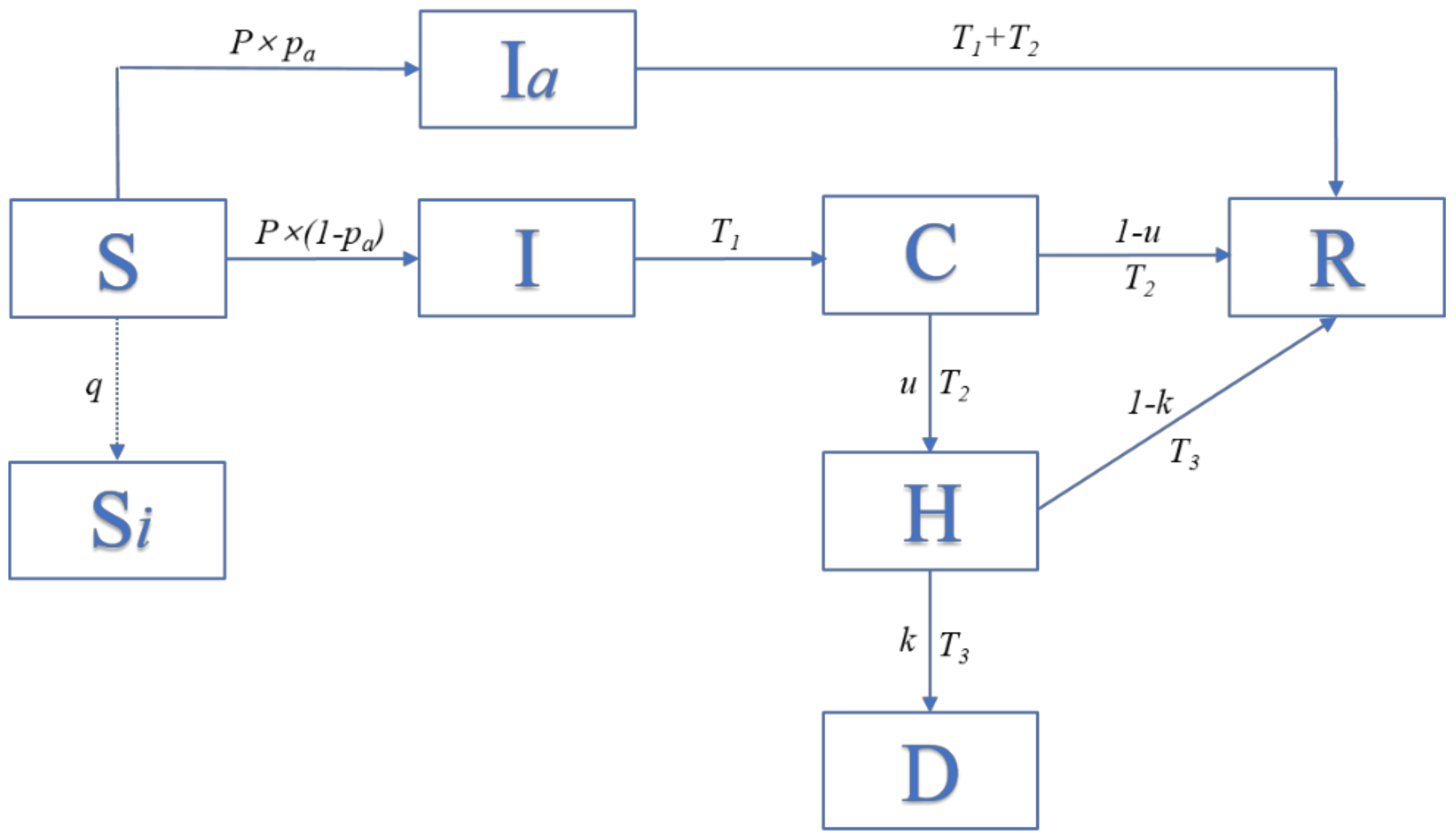
2.2. Individual Heterogeneity and the State Transition Rules

Immunity difference among individuals is defined by the following A(i, j),
A ( i , j ) = f g e n d e r × f a g e × a ( i , j )
where fgender represents the immunity coefficient related to gender, and fage represents the immunity coefficient related to age range. The values of these coefficients are determined by actual data, which are presented in Table A4 in Appendix A, and a(i, j) is assumed to follow [0,1] uniform distribution [30].
It is assumed that eight neighbors in a two-dimensional plane surround each individual, and the interaction rule with the neighbors is expressed by a transition matrix N:
N X ( i , j ) = X ( i 1 , j 1 ) X ( i 1 , j ) X ( i 1 , j + 1 )   X ( i , j 1 ) X ( i , j ) X ( i , j + 1 ) X ( i + 1 , j 1 ) X ( i + 1 , j ) X ( i + 1 , j + 1 )
where N represents the neighbor structure of X(i, j). For each individual, N is identical, which corresponds to the infection risk of certain disease. The transition of states for X(i, j) is also influenced by the current local environment, and parallel computing is exerted on every cell simultaneously.
The possibility of being infected for a susceptible individual X(i, j) at time t is defined as follows:
P ( i , j , t ) = 1 8 × ( m , n ) N X ( i , j )       m = i     o r   n = j   { P X ( i , j ) , X ( m , n ) ( t ) } + 1 8 2 × ( m , n ) N X ( i , j )       m i     a n d   n j   { P X ( i , j ) , X ( m , n ) ( t ) }
where PX(i, j) X (m, n) represents the probability of X(i, j) infected by X(m, n) at time t. The neighbors are divided into two categories by their distance: one group of neighbors are 1 away from X(i, j), the other group of neighbors are 2 away from X(i, j). Hence, the inverse of the distance is taken as the influence coefficients. The probability of being infected is inversely proportional to the resistance, and is proportional to the infectivity of its neighbors. Thus, it can be expressed as follows:
P X ( i , j ) , X ( m , n ) ( t ) = r X ( i , j ) , X ( m , n ) × ( 1 A ( i , j ) )
where rX(i, j)X(m, n) represents the infectivity of X(m, n) to X(i, j), which is also assumed to follow [0,1] uniform distribution [30]. The probability of being infected is determined by the immunity as well as the infectivity of its neighbors. Asymptomatic patient is an important character of SARS-CoV2 infections, so the parameter pa is introduced to consider the probability of becoming an asymptomatic infected individual. The set value of pa of different age groups is shown in Table A3 in Appendix A. It is worth noting that the infectivity of asymptomatic patients is half that of symptomatic ones [31].
In the beginning, infected curves of different regions present a simple rising trend; after that, the infected curves went down or presented fluctuations, which were led by different actions people took. Therefore, we introduced the parameter q to represent the people’s compliance with COVID-19 restrictions in different states to a certain degree, and it is defined as follows:
q t = 0.7 0.1 × ( C t + 1 C t ) / C t 0.025
where C represents the daily confirmed number in local actual data, qt represents the proportion of people who take effective prevention measures at time t. (Ct+1Ct)/Ct is the increase rate of confirmed numbers at time t + 1, and the increase rate at time t + 1 is related to the self-isolation proportion at time t.
The states of one individual in the cells are updated by the following:
(1)
When X(i, j, t) = 0, the possibility of being infected at time t can be calculated as mentioned above, and then, whether the individual transitions to being infected (X(i, j, t) = 3 or 8) is determined by both itself and its neighbors. If X(i, j, t) is changed from 0 to 3, then, T1(i, j, t) will be changed from 0 to 1, and the record of the infected duration of this individual begins. If X(i, j, t) is changed from 0 to 8, then T4(i, j, t) will be changed from 0 to 1, and the record of the asymptomatic infected duration of this individual begins;
(2)
When X(i, j, t) = 1 or X(i, j, t) = 2, which indicates empty positions and self-isolated individuals, respectively, their value will be constant;
(3)
When X(i, j, t) = 3 and T1(i, j, t) exceeds T1, the individual will be confirmed, and X (i, j, t) will become 4; then, T2 (i, j, t) will change from 0 to 1 and begin to record the confirmed duration, and T1(i, j, t) will return to 0;
(4)
When X(i, j, t) = 8, and T4 (i, j, t) exceeds T1 + T2, the individual will recover and X(i, j, t) will become 5; T4 (i, j, t) will return to 0;
(5)
When X(i, j, t) = 4, T2 (i, j, t) reaches T2, and the individual will be hospitalized (X(i, j, t) = 6). After obtaining hospital care, the patient may recover (X(i, j, t) = 5) with the probability of u, while probability 1 − u becomes exacerbated, the set value of u in different stage is shown in Table A5 in Appendix A;
(6)
When X(i, j, t) = 6, and T3(i, j, t) reaches T3, the infection becomes fatal (X(i, j, t) = 7) with the probability of k; otherwise, patients will recover after treatment (X (i, j, t) = 5), the set value of k in different stage is shown in Table A5 in Appendix A.
In addition to above rules, the movement of the population is correlated to the moving proportion m and the maximum moving step length L. At each time step, the states of each cell are updated simultaneously, and the movement of the individuals is simulated.
For the factor of heterogeneity, CA is suitable to demonstrate the spatial evolution of epidemics. As is shown in Figure 2, an area with size 1000 × 1000 is considered. At the initial stage, 15 infected individuals are randomly distributed in this area. The propagation process is simulated. It can be observed that the infected region (I) continues to spread outwards, while the infected individuals inside are confirmed (C) and recovered (R) after a certain time interval. In addition, the proportion of infected gradually decreases due to the increment of self-isolated (Si) proportion (q) and treatment/quarantine. The spread of infectious disease is prevented by medical response and government control. An example video is provided in the Supplementary Materials: in order to show the consideration of self-isolated individuals (Si), the self-isolation proportion is transformed artificially from 0.00 to 0.85 at around 0:55 in the video.

3. Simulation Results and Discussion

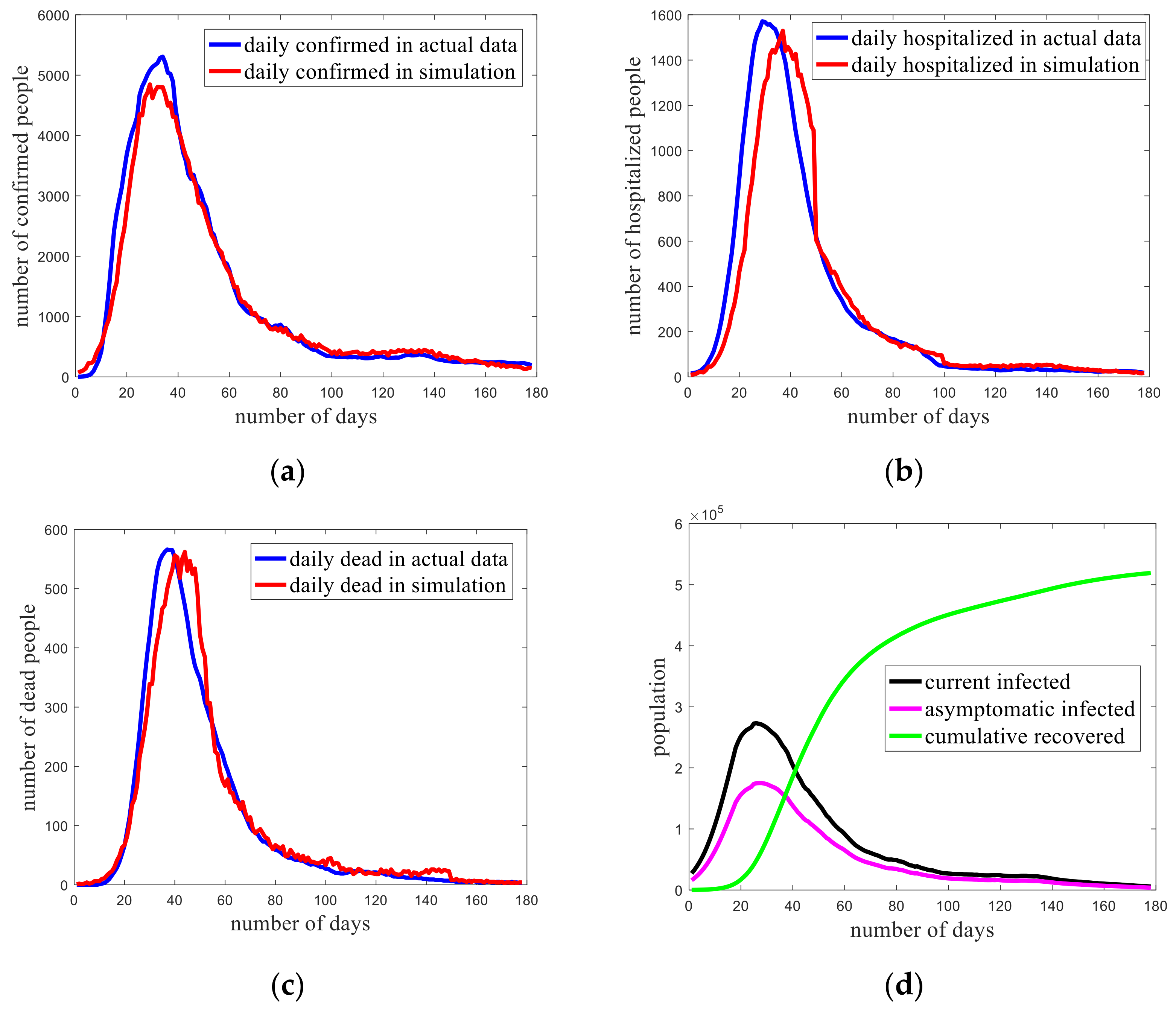
3.1. Model Verification

In order to verify proposed model, pandemic COVID-19 data from NYC and Iowa were applied. The data acquisition period ranged from 6 March to 31 August in 2020 (179 d) [32,33], and pre-processing was conducted to find the overall trend of the epidemic. In this paper, the data of daily confirmed, daily hospitalized, and daily dead were smoothed by a seven-day moving average for further application. The comparison between simulation and real data for New York and Iowa is shown in Figure 3a–c and Figure 4a. The parameters set for New York city and Iowa are presented in Table A1 and Table A2 in Appendix A, and the software used for simulation was GNU Octave 5.2.0. Robustness is very important when random factors are considered; through running the code repeatedly, it has been proven that the impact of random initial conditions on simulation results is very weak. This is an expected result for the authors, as the region size is large enough to contain the initial infected individuals, so the random distribution of initial infected individuals will always be sufficiently dispersed, which is corresponding to a robust simulation result.
As is shown in Figure 3a, the simulated number of daily confirmed rose to more than 5000 rapidly, and reached a peak at day 29 (3 April). After 3 April, the daily confirmed cases start to reduce continuously, but the descent rate is slow and the duration of the epidemic lasts for over 180 days. As control interference started around day 18 (23 March), and the self-isolation proportion (q) was added to investigate this control interference. The curves of hospitalized and dead individuals in Figure 3b,c were similar to the trend of the daily confirmed (Figure 3a), but the peak value of these two groups was far less than that of the confirmed, which reveals that most infected individuals recovered without treatment. Through a limited number of parameters (listed in Table A1), the dynamics of the epidemic are well fit, and the corresponding correlation coefficients of Figure 3a–c are 0.9912, 0.9415, and 0.9731, respectively.
The individual states considered in this model include susceptible (S), self-isolated (Si), infected (I), recovered (R), confirmed (C), hospitalized (H), and dead (D). Among them, the actual confirmed, hospitalized, and dead number can be recorded and acquired in relevant webs [32]. The trend of infected numbers and recovered numbers simulated through this model is depicted in Figure 3d, which shows that more than 500,000 individuals experienced being infected and were recovering; moreover, it also can be observed that the proportion of asymptomatic patients account for 2/3 of the overall infected individuals.
The second simulation case is the epidemic situation in Iowa. Unlike in NYC, there is still an upward trend of daily confirmed in Iowa. The number of hospitalized and dead in Iowa are negligible relative to its confirmed number; hence, only the trend of daily confirmed is concentrated. As is shown in Figure 4a, Iowa has not yet been put in place with a durably effective control strategy compared to NYC. During the 180 days after the outbreak, the phenomenon of renewed outbreaks has appeared twice in Iowa, and the daily confirmed number reaches a new peak at August 30. The self-isolation parameter q is set accordingly as shown in Figure 5, for which a correlation coefficient between simulated and actual data is as good as 0.9490. The cumulative recovered number has been more than 120,000 obtained from this model, as shown in Figure 4b.
Different states have different compliance for COVID-19 restrictions, which corresponds to different epidemic dynamic. Figure 5 shows the change curves of the self-isolation proportion (q) of NYC and Iowa, which have been validated by comparing the simulation result with actual data in Figure 3 and Figure 4. For NYC, q is set as 0 before day 18 (23 March), which means that there is no self-isolation and everyone faced the risk of being infected; after day 18 (23 March), q is set according to Equation (5). For Iowa, q is also set as 0 from day 1 to day 53 (6 March to 27 April), and set according to Equation (5) after day 53 (27 April). It can be seen that NYC presented a faster and more sustaining prevention measure than Iowa.

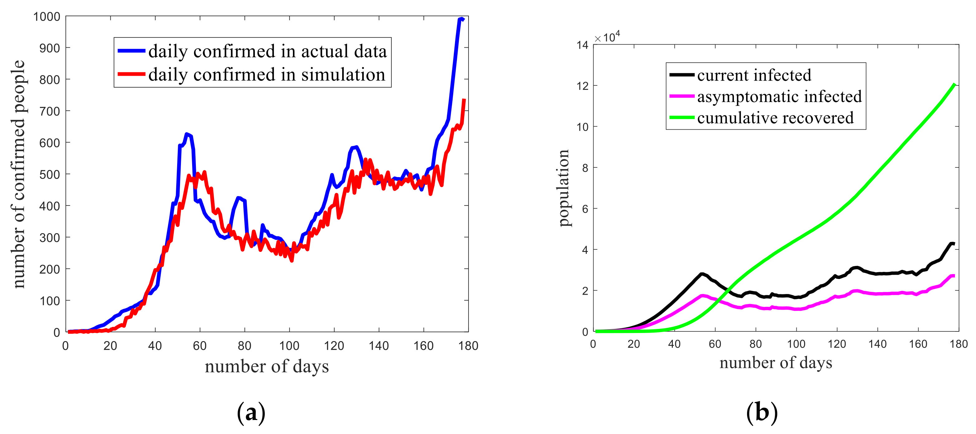
3.2. Trend Prediction of the Epidemic in Iowa

The daily confirmed number had reached 1000 in Iowa at 31 August. Based on the infection status at 31 August, the trend of infection for the next 100 days under different control strategies are simulated and exhibited in Figure 6 and Figure 7.
As shown in Figure 6a, when the self-isolation proportion is set as 0.8, which is almost the best control effect ever reached in Iowa, the daily confirmed number presents a downward trend. However, it is worth noting that only taking a long enough self-isolation period can avoid massive infection. The infection status in Iowa experienced two rebounds in the first 180 days, which may have been led by an unsustained self-isolation strategy. When the self-isolation proportion is set as 0.6, which corresponds to the middle degree of the control effect that Iowa had achieved in the past 180 d, the daily confirmed number will be stable at around 800 over the next 100 days. Obviously, this is an unfavorable outcome to prevent the infection. When q is set as 0.4, the daily confirmed number appears to have an upward trend, and reaches the peak (1315 confirmed per day) after 37 days. One positive signal is that infected number will not increase infinitely, even if the self-isolation proportion maintains at a relative low level (q = 0.4), as more and more recovered people with immunity hinder the spread. However, the cost is greater, because more individuals will be infected compared with the cases with a higher self-isolation proportion. The disturbing fact also associated with this case is that elderly people and those with underlying illness will be put in danger, which makes this case unfavorable. As shown in Figure 5b, the higher the self-isolation proportion, the less people experienced being infected during this pandemic. Although self-isolation is an effective strategy to prevent the infection and reduce the infection rate, self-isolation with a long period and wide range will lead to a large loss for local economy. In addition, the long period of self-isolation will reduce the life quality of inhabitants; therefore, a faster and more effective control strategy is needed.
Apart from self-isolation, diagnostic testing is another frequently adopted strategy to control the spread, and a combination of these two strategies can effectively shorten the duration of the epidemic. In the initial setting, only the infected individuals with symptoms will be tested and confirmed after the incubation period T1. However, for COVID-19, the infected ones within incubation period (asymptomatic) may also infect others; hence, it is necessary to take precautions to test the asymptomatic individuals periodically in order to prevent infection. In order to simulate the effect of diagnostic test during the process of infection spread, a certain proportion of individuals (including both infected and healthy) are selected randomly to be tested. The asymptomatic infected individuals and those in latency will be quarantined in advance after being tested. The test strategy is limited by the production rate of test reagent. For the same production rate of test reagent, two schemes with different intervals and scales are proposed and compared in this paper:
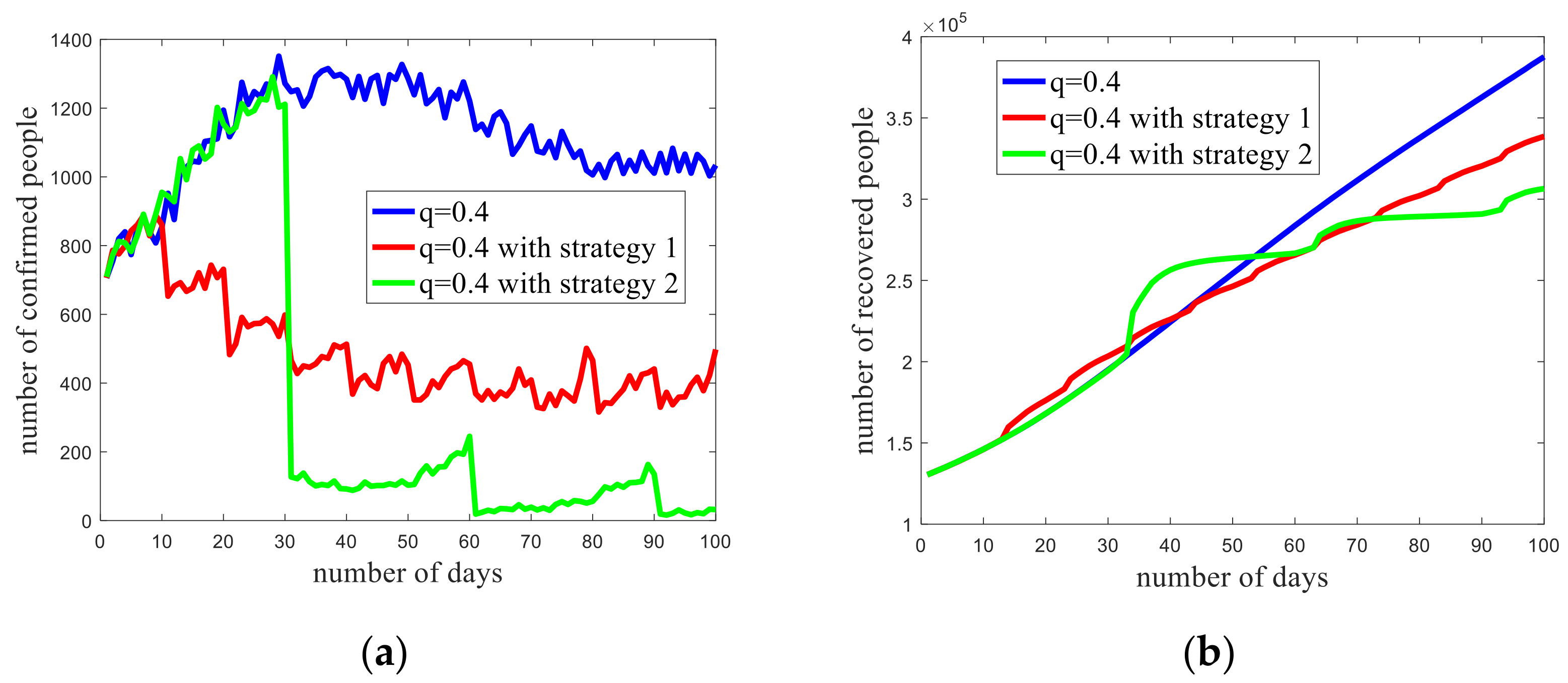
  • Test strategy 1: interval of 10 days, 30 percent of individuals are tested;
  • Test strategy 2: interval of 30 days, 90 percent of individuals are tested.
As is shown in Figure 7a, compared with the single self-isolation strategy, a combination of self-isolation and diagnostic testing results in a significant improvement in terms of infection duration and number of infected. The results present that strategy 2 is the optimal strategy (Figure 7b); strategy 1 exhibits an incomplete effect on controlling the spread of the infection, even though the test interval is the shorter than strategy 2, so the strategy with an accumulation of test reagent and large-scale collective testing is better than the strategy with frequent but small-scale testing.

4. Conclusions

A CA model for simulating and analyzing epidemic evolution is proposed in this paper. Through this model, a simplified social community is considered and expressed on a two-dimensional plane, and individual heterogeneity is considered with parameters including sex ratio, age structure, individual immunity, incubation and treatment period, and population movement. COVID-19 confirmation data from NYC and Iowa are adopted for model validation purposes, and the number of confirmed in Iowa is predicted with different control strategies. It is shown that a synergistic action of self-isolation and diagnostic testing can effectively prevent the spread of infectious diseases. In addition, the test strategy with a long interval and larger scale is better than that with short interval and small scale when the production capacity of test reagent is limited.
The authors sincerely hope this work can provide an alternative to study the spread of infectious disease, and eventually help to control any infection across the world in the future. Based on the model established in this work, more actual strategies can be investigated to better facilitate decision-making, including partitioned management and multi-strategy synergy. Besides infection issues, symptoms could be much more diverse, corresponding to the change of infection mechanism. It is also helpful and feasible to identify the evolution state of the spread based on data analysis from systematic point of view. The spread of all infectious diseases within a certain region can be studied as a complex system with an inherent mechanism in future study.

Supplementary Materials

The following are available online at https://www.mdpi.com/2227-9717/9/1/55/s1, Video S1: Figure 2.mp4, Source code S1: NYC.m, IA.m, IApredict.m, IAtest1.m, IAtest2.m and qcurve.m.

Author Contributions

Conceptualization, W.S., J.W., and J.A.; methodology, J.D.; software, J.W.; validation, W.S. and C.Z.; formal analysis, C.Z.; investigation, J.M. and J.A.; resources, W.S.; data curation, J.D.; writing—Original draft preparation, J.D.; writing—Review and editing, W.S.; visualization, J.D. and J.M.; supervision, W.S.; project administration, C.Z.; funding acquisition, W.S. All authors have read and agreed to the published version of the manuscript.

Funding

The authors gratefully acknowledge the following institutions for support: The National Natural Science Foundation of China (Grant No. 21878012).

Institutional Review Board Statement

Not applicable.

Informed Consent Statement

Not applicable.

Data Availability Statement

The data presented in this study are available in supplementary material.

Conflicts of Interest

The authors declare no conflict of interest. The funders had no role in the design of the study, in the collection, analyses, or interpretation of data, in the writing of the manuscript, or in the decision to publish the results.

Appendix A

The parameters set for NYC and Iowa are presented below. The parameters in the proposed model can be divided into two types: one kind of parameter is the characteristic parameter for infectious diseases (including infection period T1, confirmed period T2, treatment period T3, vacancy ratio α, moving proportion m, maximum moving step length L, immunity coefficient f, hospitalization fraction u, and dead fraction k). In this paper, this kind of parameter is determined by the confirmation data from NYC and verified by the confirmation data from Iowa. Among the parameters, vacancy ratio α, moving proportion m, and maximum moving step length L do not seem like the disease characteristic parameters, but in fact, these three parameters determine that an infected individual will have contact with a certain number of individuals. This has a similar concept named basic regeneration number R0, and R0 is generally fixed for one particular infection [34]. Immunity coefficient f is a special disease characteristic parameter, because its value is determined by the data analysis—from [32], the rate of confirmed cases per 100,000 people by sex and the rate of confirmed cases per 100,000 people by age group can be obtained, so that the immune coefficient can be set accordingly. For example, the proportion of immune coefficients for males and females is equal to the proportion of infected for males and females. The other kind of parameters are the characteristic parameters of the region in consideration (including the initial number of infected ε, sex ratio gsex, age structure gage, and self-isolation proportion q), which can be determined by local related data.
Table A1. The parameters set for NYC.
SymbolDescriptionValue
nRegion size1000.000
αVacancy ratio0.200
εInitial number of infected (on 15 February)250.000
T1Period from infected to confirmed10.000
T2Period from confirmed to hospitalized4.000
T3Period from hospitalized to recovered4.000
mMoving proportion0.160
LMaximum moving step length10.000
gmaleMale proportion0.477
gfemaleFemale proportion0.523
gage > 60Proportion of the elderly0.170
gage < 60Proportion of the younger0.830
Table A2. The parameters set for Iowa.
SymbolDescriptionValue
nRegion size1000.000
αVacancy ratio0.200
εInitial number of infected (on 29 February)20.000
T1Period from infected to confirmed10.000
T2Period from confirmed to hospitalized4.000
T3Period from hospitalized to recovered4.000
mMoving proportion0.160
LMaximum moving step length10.000
gmaleMale proportion0.495
gfemaleFemale proportion0.505
gage > 60Proportion of the elderly0.240
gage < 60Proportion of the younger0.760
Table A3. The probability of becoming an asymptomatic patient (pa) for different age groups [31].
Age Range0–45–1415–2930–5960–6970–7980–
pa0.950.80.70.50.40.30.2
Table A4. The set value of the immunity coefficient.
Immune CoefficientDescriptionValue
fmaleImmunity coefficient for male individuals0.8059
ffemaleImmunity coefficient for female individuals1.0000
fage > 60Immunity coefficient for old individuals0.7673
fage < 60Immunity coefficient for young individuals1.0000
Table A5. The set value for the hospitalization fraction (u) and dead fraction (k).
Data Rangeuk
6 March to 23 April0.310.38
24 April to 12 June0.180.33
13 June to 1 August0.120.42
after 1 August0.110.17

References

  1. The World Health Report 2013. Available online: https://www.who.int/publications/i/item/9789240690837 (accessed on 20 October 2020).
  2. Andrews, J.R.; Basu, S. Transmission dynamics and control of cholera in Haiti: An epidemic model. Lancet 2011, 377, 1248–1255. [Google Scholar] [CrossRef] [Green Version]
  3. Cooper, B.S.; Lipsitch, M. The analysis of hospital infection data using hidden Markov models. Biostatistics 2004, 5, 223–237. [Google Scholar] [CrossRef] [PubMed] [Green Version]
  4. Brossette, S.E.; Sprague, A.P.; Hardin, J.M.; Waites, K.B.; Jones, W.T.; Moser, S.A. Association Rules and Data Mining in Hospital Infection Control and Public Health Surveillance. J. Am. Med. Inform. Assoc. 1998, 5, 373–381. [Google Scholar] [CrossRef] [PubMed] [Green Version]
  5. Anderson, S.; Harper, L.M.; Dionne-Odom, J.; Halle-Ekane, G.; Tita, A.T.N. A decision analytic model for prevention of hepatitis B virus infection in Sub-Saharan Africa using birth-dose vaccination. Int. J. Gynecol. Obstet. 2018, 141, 126–132. [Google Scholar] [CrossRef] [PubMed]
  6. Kermack, W.O.; McKendrick, A.G. A contribution to the mathematical theory of epidemics. Proc. R. Soc. Lond. Ser. A Math. Phys. Sci. 1927, 115, 700–721. [Google Scholar]
  7. Duque, D.; Morton, D.; Singh, B.; Du, Z.; Pasco, R.; Meyers, L.A. Timing social distancing to avert unmanageable COVID-19 hospital surges. Proc. Natl. Acad. Sci. USA 2020, 117, 19873–19878. [Google Scholar] [CrossRef]
  8. Biswas, H.A.; Paiva, L.T.; De Pinho, M.D.R. A SEIR model for control of infectious diseases with constraints. Math. Biosci. Eng. 2014, 11, 761–784. [Google Scholar] [CrossRef]
  9. Liu, J.; Zhang, T. Epidemic spreading of an SEIRS model in scale-free networks. Commun. Nonlinear Sci. Numer. Simul. 2011, 16, 3375–3384. [Google Scholar] [CrossRef]
  10. Naresh, R.; Sharma, D.; Tripathi, A. Modelling the effect of tuberculosis on the spread of HIV infection in a population with density-dependent birth and death rate. Math. Comput. Model. 2009, 50, 1154–1166. [Google Scholar] [CrossRef]
  11. Srivastava, P.K.; Banerjee, M.; Chandra, P. A Primary Infection Model for HIV and Immune response with Two Discrete Time Delays. Differ. Equ. Dyn. Syst. 2010, 18, 385–399. [Google Scholar] [CrossRef]
  12. Simons, E.; Ferrari, M.; Fricks, J.; Wannemuehler, K.; Anand, A.; Burton, A.; Strebel, P. Assessment of the 2010 global measles mortality reduction goal: Results from a model of surveillance data. Lancet 2012, 379, 2173–2178. [Google Scholar] [CrossRef]
  13. Watanabe, T.; Bartrand, T.A.; Weir, M.H.; Omura, T.; Haas, C.N. Development of a Dose-Response Model for SARS Coronavirus. Risk Anal. 2010, 30, 1129–1138. [Google Scholar] [CrossRef] [PubMed] [Green Version]
  14. Kerr, C.C.; Stuart, R.M.; Gray, R.T.; Shattock, A.J.; Fraser-Hurt, N.; Benedikt, C.; Haacker, M.; Berdnikov, M.; Mahmood, A.M.; Jaber, S.A.; et al. Optima. JAIDS J. Acquir. Immune Defic. Syndr. 2015, 69, 365–376. [Google Scholar] [CrossRef] [PubMed]
  15. De La Sen, M.; Alonso-Quesada, S. Vaccination strategies based on feedback control techniques for a general SEIR-epidemic model. Appl. Math. Comput. 2011, 218, 3888–3904. [Google Scholar] [CrossRef]
  16. Sun, C.; Lin, Y.; Tang, S. Global stability for an special SEIR epidemic model with nonlinear incidence rates. Chaos Solitons Fractals 2007, 33, 290–297. [Google Scholar] [CrossRef]
  17. Elaiw, A.M.; Alshamrani, N.H. Global stability of a delayed humoral immunity virus dynamics model with nonlinear incidence and infected cells removal rates. Int. J. Dyn. Control. 2015, 5, 381–393. [Google Scholar] [CrossRef]
  18. Dezső, Z.; Barabási, A.-L. Halting viruses in scale-free networks. Phys. Rev. E 2002, 65, 055103. [Google Scholar] [CrossRef] [Green Version]
  19. Ferdinandy, B.; Mones, E.; Vicsek, T.; Müller, V. HIV Competition Dynamics over Sexual Networks: First Comer Advantage Conserves Founder Effects. PLoS Comput. Biol. 2015, 11, e1004093. [Google Scholar] [CrossRef] [Green Version]
  20. Firth, J.A.; Hellewell, J.; Klepac, P.; Kissler, S.M.; Kucharski, A.J.; Spurgin, L.G. Using a real-world network to model localized COVID-19 control strategies. Nat. Med. 2020, 26, 1616–1622. [Google Scholar] [CrossRef]
  21. Jiang, Z.; Hu, M.; Fan, L.; Pan, Y.; Tang, W.; Zhai, G.; Lu, Y. Combining Visible Light and Infrared Imaging for Efficient Detection of Respiratory Infections such as COVID-19 on Portable Device. arXiv 2020, arXiv:2004.06912. [Google Scholar]
  22. Neumann, J.V.; Burks, A.W. Theory of Self-Reproducing Automata; University of Illinois Press: Champaign, IL, USA, 1966; Available online: https://science.sciencemag.org/content/157/3785/180.1 (accessed on 20 October 2020).
  23. Kleingeld, P.; Brown, E. The Stanford Encyclopedia of Philosophy; Stanford University Press: Palo Alto, CA, USA, 2012; Available online: https://plato.stanford.edu/ (accessed on 20 October 2020).
  24. White, S.H.; Del Rey, A.M.; Sánchez, G.R. Modeling epidemics using cellular automata. Appl. Math. Comput. 2007, 186, 193–202. [Google Scholar] [CrossRef] [PubMed]
  25. Athithan, S.; Shukla, V.P.; Biradar, S.R. Dynamic Cellular Automata Based Epidemic Spread Model for Population in Patches with Movement. J. Comput. Environ. Sci. 2014, 2014, 518053. [Google Scholar] [CrossRef] [Green Version]
  26. Pfeifer, B.; Kügler, K.; Tejada, M.M.; Baumgartner, C.; Seger, M.; Osl, M.; Netzer, M.; Handler, M.; Dander, A.; Wurz, M.; et al. A Cellular Automaton Framework for Infectious Disease Spread Simulation. Open Med. Inform. J. 2008, 2, 70–81. [Google Scholar] [CrossRef]
  27. Holko, A.; Mȩdrek, M.; Pastuszak, Z.; Phusavat, K. Epidemiological modeling with a population density map-based cellular automata simulation system. Expert Syst. Appl. 2016, 48, 1–8. [Google Scholar] [CrossRef]
  28. Mikler, A.R.; Venkatachalam, S.; Abbas, K. Modeling infectious diseases using global stochastic cellular automata. J. Biol. Syst. 2005, 13, 421–439. [Google Scholar] [CrossRef]
  29. López, L.; Burguerner, G.; Giovanini, L. Addressing population heterogeneity and distribution in epidemics models using a cellular automata approach. BMC Res. Notes 2014, 7, 234. [Google Scholar] [CrossRef] [Green Version]
  30. Bin, S.; Sun, G.; Chen, C.C. Spread of infectious disease modeling and analysis of different factors on spread of infectious disease based on cellular automata. Int. J. Public Health 2019, 16, 4683. [Google Scholar] [CrossRef] [Green Version]
  31. Röst, G.; Bartha, F.A.; Bogya, N.; Boldog, P.; Dénes, A.; Tamás, F.; Horváth, K.J.; Juhász, A.; Nagy, C.; Tekeli, T.; et al. Early Phase of the COVID-19 Outbreak in Hungary and Post-Lockdown Scenarios. Viruses 2020, 12, 708. [Google Scholar] [CrossRef]
  32. The Coronavirus Disease 2019 (COVID-19) Data in New York City. Available online: https://github.com/nychealth/coronavirus-data (accessed on 20 October 2020).
  33. The Coronavirus Disease 2019 (COVID-19) Data in Iowa. Available online: https://coronavirus.iowa.gov/ (accessed on 20 October 2020).
  34. Driessche, P.V.D.; Watmough, J. Reproduction numbers and sub-threshold endemic equilibria for compartmental models of disease transmission. Math. Biosci. 2002, 180, 29–48. [Google Scholar] [CrossRef]
Figure 1. The state transition mechanism.
Processes 09 00055 g001
Figure 2. An example to present the epidemic spatial evolution (time (t) = 20, 60, and 120 d).
Processes 09 00055 g002
Figure 3. (a) The comparison result of New York City (NYC) in terms of daily confirmed. (b) The comparison result of NYC in terms of daily hospitalized. (c) The comparison results of NYC in terms of daily dead. (d) The trend of infected numbers and recovered numbers.
Processes 09 00055 g003
Figure 4. (a) The comparison result of Iowa in terms of daily confirmed. (b) The trend of the number of infected and recovered in Iowa.
Processes 09 00055 g004
Figure 5. The change curve of self-isolation proportion (q) of NYC and Iowa (IA).
Processes 09 00055 g005
Figure 6. (a) Simulation results of Iowa under different self-isolated proportions (q). (b) The trend of recovered number under different self-isolated proportions (q).
Processes 09 00055 g006
Figure 7. (a) Simulation results of Iowa under different diagnostic test strategies (different test strategies have different intervals and scales). (b) The trend of the number of recovered corresponding to different strategies.
Processes 09 00055 g007
Publisher’s Note: MDPI stays neutral with regard to jurisdictional claims in published maps and institutional affiliations.

