A Model of Transport of Particulate Biomass in a Stream of Fluid

Abstract

The motion of a solid particle introduced into a stream of fluid is a crucial problem in the contexts of pneumatic transport and the purification and separation of non-uniform mixtures. However, the complexity of the underlying equations of motion enforces the creation of semi-empirical models. Therefore, analysis of particle motion in a pneumatic channel was performed. To reduce the number of independent variables, several simplifying assumptions were made in regard to both the particle and the stream. The resulting model provides trajectory equations for a particle introduced into the stream at given values of the initial angle and initial velocity, which are then solved using numerical integration methods. A hodograph function was formulated on the basis of the Runge–Kutta and NDFs methods to test the correctness of the solutions under various initial parameters and to provide a universal method of solving the equations of motion. To verify the model, terminal velocities were measured and particle trajectories recorded using an original experimental stand. The predictions of the model were subsequently compared to these empirical trajectories and were found to fall within the range of uncertainty.

1. Introduction

The topic of modeling the movement of particles in a stream of fluid is a crucial one in the context of the process of pneumatic transport, as well as the purification and separation of non-homogeneous mixtures [1,2]. These processes appear in many branches of industry, such as coal mining [3], environment and waste management [4], as well as agriculture and the food industry [5,6,7], with additional weight given to this problem by the huge quantity of materials involved. Such a model, if developed properly, may then be used to bolster these processes by predicting the behavior of the processed material during their course.

Qualities such as shape, surface texture, and the mass of the particles are inherently tied to their hydrodynamical properties. This allows them to be used as discriminatory traits for the separation of particles of similar sizes, which cannot be fully achieved by other means [8,9,10]. This method, known as pneumatic separation [4,5], is particularly important whenever significant differences in shape and mass, coupled with relatively similar particle sizes, occur between the desired material and the waste. This is commonly the case in the agriculture industry (e.g., grain versus chaff and shells), but also in the sortition of particulate biomass for the purposes of renewable energy production and waste management. For this reason, pneumatic separation is valued both as the primary and secondary method of separation [11,12,13].

The complexity of hydrodynamics equations significantly complicates any theoretical description of the processes of pneumatic transport and separation. It is thus virtually required for any model to be based on experimentally measured parameters, such as critical (terminal) velocity [14,15]. However, a fair comparison is only possible between disparate works and different experimental conditions when a complete nondimensional analysis is also provided. Unfortunately, in a majority of cases, the state of the research only involves exploratory studies of specific separators. An example might be given in the case of the studies by Nesterenko et al. [16], who tested a prototype separator over several operating conditions, but the resulting quantitative data was only applicable in the context of that specific prototype. A similar lack of the possibility of broader application is found in a paper by Tobias et al. [17]. Exploratory studies have also been performed by Panasiewicz et al. [9], who assessed the influence of humidity, particle size, and air velocity on separation efficiency. Although the authors declared that their results allowed the calculation of the pneumatic parameters for various constituent particles, they did not provide any examples of such. A much better theoretical background is to be found in Badretdinov et al. [18], who provided a description of a general circulation model (GCM) as a complex system of multi-dispersionary two-phase air–solid flow, accounting for gravity, friction, and drag forces, but did not account for the angle of introduction of the material into the stream. This was amended by Stepanenko and Kotov [19], who proposed a model of interaction between the particle and mass flow, expressed in terms of a set of differential equations, but did not describe the solid particle. Moreover, Stepanenko and Kotov did not provide solutions to their equations, nor did they verify their model experimentally. Therefore, their veracity is unknown.

Computer modeling is an acknowledged method in studies of particulate matter. An example of such an in silica approach in the context of the processing of agricultural products can be found, for example, in Kryszak et al. [20].

A particle in a stream of fluid is subject to the force of aerodynamic drag R, the force of gravity G, and the buoyant force W. Due to the very low density of air compared with the densities of solid bodies, the buoyant force may usually be neglected. Therefore, the behavior of a particle in a stream of air is determined by the drag force and gravity.

The simplest case occurs when drag and gravity act in the same direction and the particle’s entire movement occurs in one dimension, such as when a particle is in freefall in a stream that is moving vertically upward. The behavior of the particle may take three forms:

• The stream velocity v_f is low enough that G > R and the particle falls with velocity v (Figure 1a);
• The drag overcomes gravity, G < R, and the particle is lifted by the stream (Figure 1b);
• The forces acting on the particle balance each other and it remains in place (Figure 1c).

The last of these, as a boundary case, is crucial for the theory of pneumatic separation of mixtures; the velocity of the stream at which this happens is known as the critical (terminal) velocity. While it is usually defined as the greatest velocity that is achieved by a body falling freely in a non-vacuous medium [21], it is measured in relation to the stream of fluid the body moves through, which makes both definitions equivalent.

The relation describing the critical velocity may be derived from the equilibrium condition, assuming the relative velocity of a particle v_w = v_f = v_c (since v = 0):

v_c = (2mg/c_xAρ_f)^1/2

(1)

where v_c is the critical velocity for the stream (m/s), c_x is the aerodynamic drag coefficient (-), ρ_f is the density of the fluid (air) (kg/m³), A is the projected area of the particle along the direction of movement (m²), m is the mass of the particle (kg), and g is Earth’s gravity (m/s²).

Under uniform external conditions, the critical velocity depends solely on the particle’s properties, including its texture and shape. Because of that, this quantity is considered to be the primary parameter characterizing the aerodynamic properties of a particle. By knowing its value, one may predict the behavior of a particle in a stream. All particles characterized by a critical velocity lower than the velocity of the stream will be lifted, while those of a higher velocity will fall. Since a falling particle of a non-isotropic shape will naturally assume the position of the lowest drag, the critical velocity must be measured empirically.

Drag R is defined by Equation (2) [22,23]:

R = −0.5 (c_xAρ_f|v_w|) v_w

(2)

where v_w is the relative velocity of the particle in respect to the stream and is of a value defined by the following equation:

v_w = ((v_x − v_fx)² + (v_y − v_fy)²)^1/2

(3)

where v_{x,y} is the velocity of the particle in the direction {x, y} (m/s) and v_{f {x,y}} is the velocity of the fluid in the direction {x, y} (m/s).

The drag coefficient c_x is dependent on the Reynolds number which, in cases of forced flow, is defined by the following equation:

Re = v_wd/ν_f

(4)

where d is the diameter of the particle (m) and ν_f is the kinematic viscosity of the fluid (s/m²).

The drag force may be split into vertical and horizontal components:

R = R cosγ ˆx = 0.5 (c_xAρ_f |v_w|) (v_fx − v_x)

(5)

R = R cosγ ˆy = 0.5 (c_xAρ_f |v_w|) (v_fx − v_x)

(6)

where γ is the angle between the drag force vector and the horizontal axis and ˆx, ˆy are the unit vectors.

The movement of solid particles in a fluid medium is the domain of a subsection of fluid mechanics known as two-phase flow mechanics. In this area of study, an early theoretical model of unsteady movement in a steady fluid velocity field was provided by Orzechowski [22]. This model supposes a range of simplifications and assumptions, chief among them being the following:

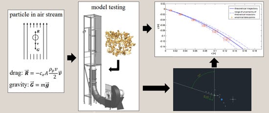
• The particles are spheres of a diameter d;
• The fluid fills unlimited space;
• The stream flows along straight lines.

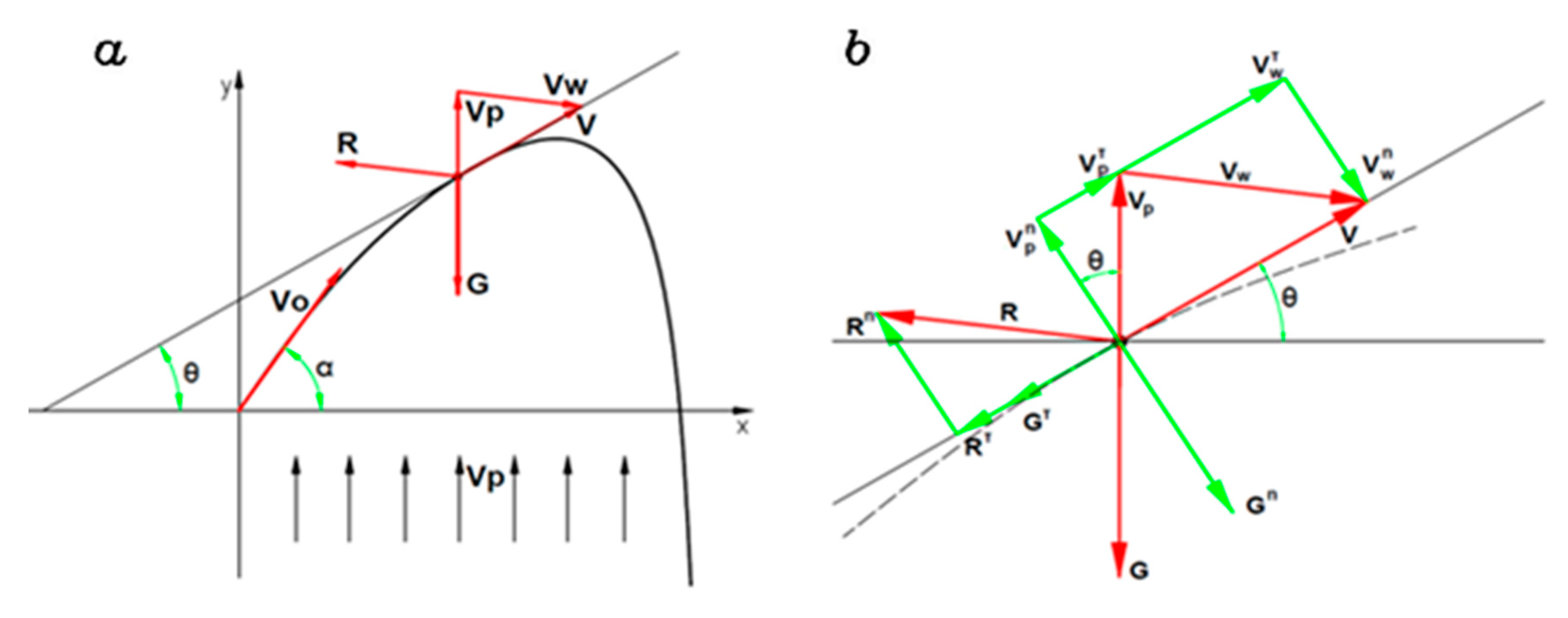
The following forces act on a particle in a stream of fluid (Figure 2a):

• Drag force R;
• Apparent weight G (weight minus buoyancy);
• Inertial force F.

The fluid moves at a velocity v_f, while the particle is described by the absolute velocity v and the relative velocity v_w (Figure 2b).

On the basis of Equations (5) and (6), the dynamic equations of motion assume the following form:

m(dv_x/dt) = 0.5 (c_xAρ_f v_w) (v_fx − v_x)

(7)

m(dv_y/dt) = 0.5 (c_xAρ_f v_w) (v_fy − v_y) + Vg (ρ − ρ_f)

(8)

where g is Earth’s gravity ≈ 9.81 m/s², ρ is the density of the particle (kg/m³), and V is the volume of the particle (m³).

In addition, the mass of the particle may include the mass of water bound to the particle’s surface, according to the following equation:

m = V (ρ + ϕρ_f)

(9)

where ϕ is an empirical parameter denoting the amount of fluid moving along with the particle (-).

In cases where a closer description of the shape of a particle is necessary, one may introduce a parameter of sphericity, such as that provided by Mohsenin [24]:

Ψ = (abc)^1/3/c

(10)

where a, b, c are the particle dimensions along each axis (c > a, b).

In order to solve Equations (7) and (8), one needs to know the drag coefficient, which is dependent on Reynolds number. This relation has an approximately linear characteristic for Reynolds numbers below 0.4, non-linear for values between 0.4 and 2∙10⁵, and constant for higher values [24,25]. Various models have been created to calculate the value of the drag coefficient. In the context of pneumatic separation, the most commonly used one is the Kaskas model [23]:

c_x = 24/Re + 4/Re^1/2 + 0.4

(11)

Applying the Kaskas model to Equations (7) and (8) produces a set of non-linear equations. As their analytical solution is non-trivial, a simpler model is sought. Orzechowski proposes a model solvable for laminar flow, but its applicability is limited by the comparative rarity of such cases under non-laboratory conditions [20]. Panasiewicz assumes the uniform and unbound flow of a fluid (air) with a particle introduced into it at a given initial velocity [8]. Since the Reynolds number for such a flow is high, he assumed a constant drag coefficient, which allowed him to provide a parametric equation of motion in respect to the angle between the particle velocity vector and the horizontal axis:

t = ∫^θ _θ0 (kg)^−1/2 cos⁻²θ {sinθ/cos²θ − sinθ₀/cos²θ₀ + ln[tan(θ/2 + π/4)/tan(θ₀/2 + π/4)]
− g/(kv²_w0 cos²θ₀) }^−1/2 dθ

(12)

x’ = ∫^θ _θ0 k/cos²θ {sinθ/cos²θ − sinθ₀/cos²θ₀ + ln[tan(θ/2 + π/4)/tan(θ₀/2 + π/4)]
− g/(kv²_w0 cos²θ₀) }⁻¹ dθ

(13)

y’ = ∫^θ _θ0 k(tanθ/cos²θ) {sinθ/cos²θ − sinθ₀/cos²θ₀ + ln[tan(θ/2 + π/4)/tan(θ/2 + π/4)]
− g/(kv²_w0 cos²θ₀) }⁻¹ dθ

(14)

where θ₀ is the initial angle (i.e., the angle between the initial particle velocity and the horizontal axis), v_w0 is the initial relative velocity of a particle, and k is a parameter equal to

k = c_xAρ_f/2m = v_c²/g = 1/k₀

(15)

where k₀ is the volatility parameter of the particle [26].

However, he provided neither a general solution, nor a transformation to the Cartesian coordinates.

Therefore, the aim of the research presented in this paper was to produce a model of movement of a particle in a pneumatic channel that improves upon previous models and provide its subsequent verification in laboratory conditions.

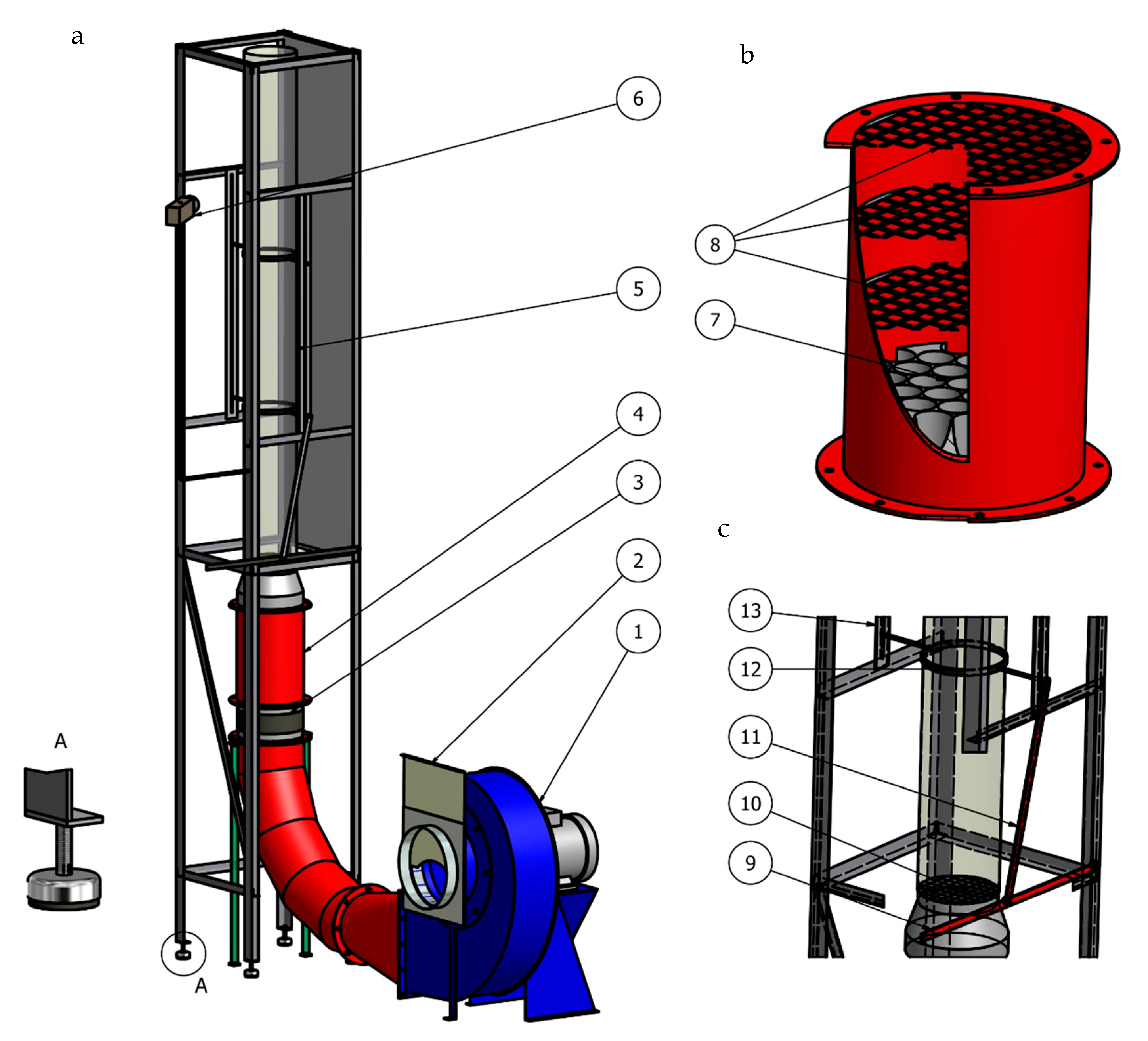
2. Materials and Methods

Figure 3 presents the chief factors influencing the aerodynamic properties of a particle. Among these, the most decisive are the shape and size (which determine the size of the projected area), as well as the mass of the particle. However, mixtures found in agriculture and renewable resource management often consist of particles of highly varied shapes and sizes, which makes their quantitative description difficult. As it has been the topic of much research, one may encounter a wide variety of proposed solutions. For example, in the case of plant-derived particles, Frączek and Wróbel [27] point out three broad methods of shape assessment: conflating them with simple geometric objects, introducing a shape coefficient, and virtual models.

The above analysis forms a foundation for a mathematical model of the process. Since the number of possible independent parameters is huge, the model should include only the most crucial ones, with the less important parameters assumed to be constant in order to reduce potential uncertainty. With this in mind, the case was simplified by making the following assumptions:

• The density and dynamic viscosity of the air are constant;
• The air velocity distribution is flat along a given cross-section of the pneumatic channel;
• The fluctuating component of the velocity is negligible;
• The solid particle is spherical, with a diameter d, mass m, and drag coefficient c_x;
• The solid particle does not rotate along its axis and remains in thermodynamic equilibrium with the air;
• The drag coefficient is constant;
• The mass of the layer of air accompanying the particle and the buoyant force are negligibly small;
• The boundary effects pertaining to the walls of the pneumatic channel have no influence on the particle;
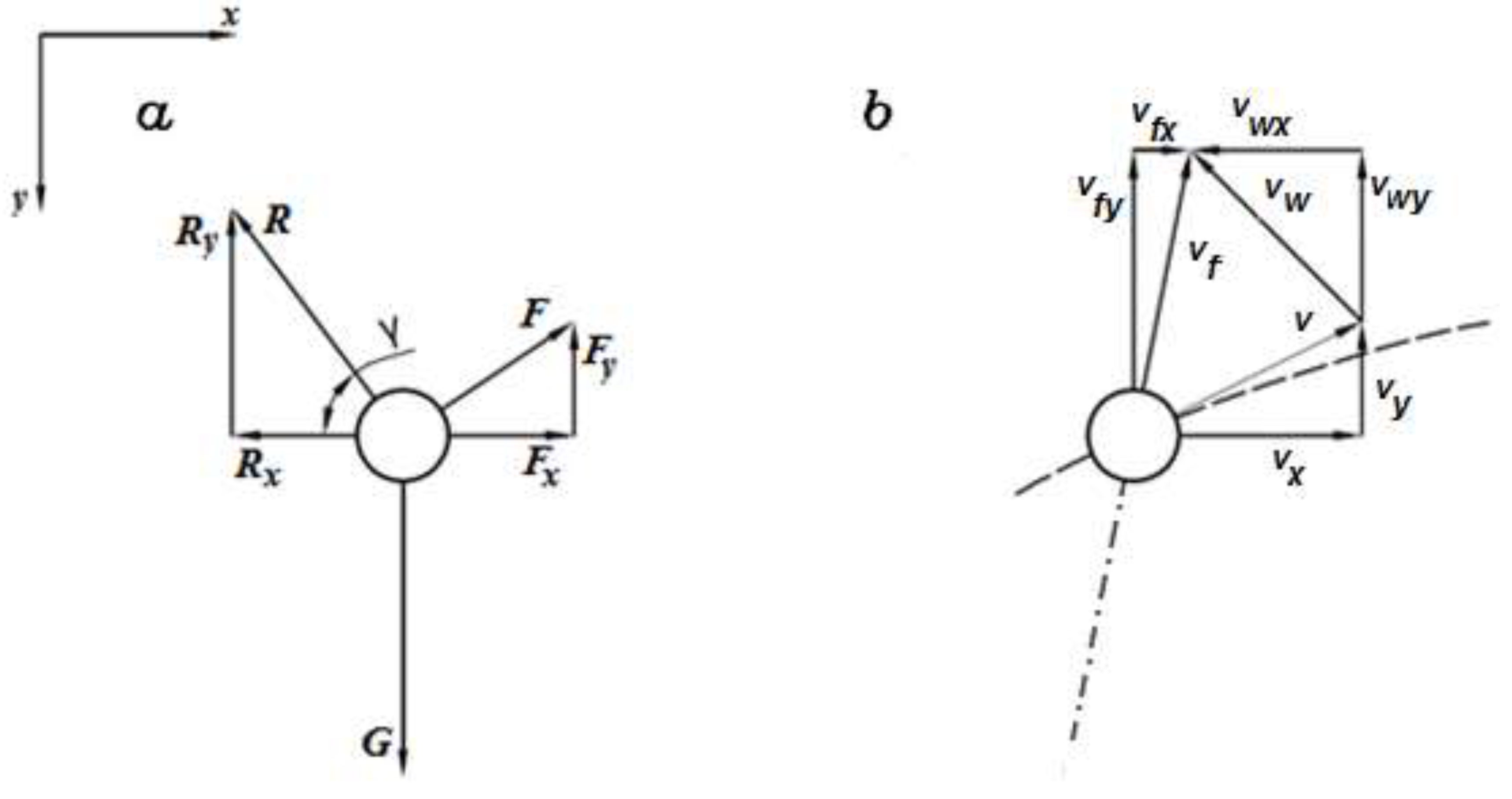
• The particle is introduced into the pneumatic channel with a velocity of a known value v₀ at an angle α in respect to the horizontal level (Figure 4a);
• The particle’s movement, determined by gravity and drag, occurs on a single plane.

The frame of reference is fixed in the place of introduction of the particles into the channel, the x axis is horizontal, and the y axis vertical (Figure 4a). The limit to motion posed by the walls of the channel was also omitted at this point.

In the simplest case, the stream of air is vertical and directed upward (Figure 4). If the channel is large enough for it to be treated as unbounded, the particle is introduced at a velocity v₀ at an angle α in respect to the horizontal axis, taking into account that the tangent to the trajectory at any given point is tilted against the horizontal level at an angle θ. The scalar equations of motion take the following forms:

ma_N = mgcosθ − 0.5 c_xAρ_f |v_w| v_fN,

(16)

ma_T = mgsinθ − 0.5 c_xAρ_f |v_w| v_fT

(17)

where a_N is the normal acceleration, defined as

a_N = v²/r = − v (dθ/ds)(ds/dt) = − v dθ/dt

(18)

where a_T is the tangential acceleration, defined as

a_T = dv/dt = (dv/dθ)(dθ/dt)

(19)

where v_wN is the relative normal velocity of the particle, v_wT is the relative tangential velocity of the particle (defined as the change in the position of the particle over time), and θ is the angle between the tangent and the horizontal axis.

Inserting Equations (18) and (19) into Equations (16) and (17), they may be reduced to a single equation, which can be further simplified by using the critical (terminal) velocity formula in Equation (1):

dv/dθ = v (v_c² sinθ + |v_w|v_wT)/(v_c² cosθ − |v_w|v_wN).

(20)

The components of the relative particle velocity vector can be derived from Figure 4b:

v_wN = v_fN = v_f cosθ,

(21)

v_wT = v − v_fT = v − v_f sinθ

(22)

The relative velocity has the following value:

|v_w| = (v_f² + v² − 2v_fv sinθ)^1/2

(23)

Taking the above in account, Equation (21) takes the following form:

dv/dθ = (v/cosθ)[v_c²sinθ + (v − v_ysinθ)(v_f²+v²–2v_fvsinθ)^1/2]/[v_c² − v_f (v_f²+v²–2v_fvsinθ)^1/2]

(24)

Assuming the initial conditions θ = α and v = v₀ (i.e., the initial point of movement), one achieves the solution to Equation (24): the hodograph function of the absolute velocity vector with respect to θ:

v = f(θ)

(25)

By applying Equation (18) to Equation (16) and subsequently separating the variables and reformulation, the latter equation takes the following form:

dt = (v/g) (|v_w|v_wN/v_c² − cosθ)⁻¹ dθ

(26)

From this, one reaches the following:

dt = f(θ)/(gcosθ) [(v_f/v_c²)(v_f² + v² − 2v_fvsinθ)^1/2 − 1]⁻¹ dθ

(27)

By integrating this equation under the assumption that, at the initial point of movement (i.e., t = 0), the angle θ equals α, one receives

t = ∫^θ _α {f(θ)/(gcosθ) [(v_f/v_c²)(v_f² + v² − 2v_fvsinθ)^1/2 − 1]⁻¹} dθ

(28)

The generalized equations of motion are taken to assume the following form for t = 0, x = 0, and y = 0:

x = ∫^t ₀ v cosθ dθ

(29)

y = ∫^t ₀ v sinθ dθ

(30)

By applying the relation in Equation (28) to the above and changing the integration parameters (θ = α for t = 0), one achieves the solution for parametric equations of motion in a vertical stream of air:

x = ∫^θ _α {f²(θ)/g [(v_f/v_c²)(v_f² + f²(θ) − 2v_f sinθ f(θ))^1/2 − 1]⁻¹} dθ

(31)

y = ∫^θ _α {f²(θ)tanθ/g [(v_f/v_c²)(v_f² + f²(θ) − 2v_f sinθ f(θ))^1/2 − 1]⁻¹} dθ

(32)

This result can be generalized for any stream of air tilted against the vertical direction at an angle β (such as in a tilted pneumatic channel) (Figure 4a).

From the distribution of the force and velocity vectors (Figure 4b), it is not hard to see that only the relative velocity vector was changed in respect to the vertical stream. Its components and value assume the following form:

v_wN = v_fN = v_f cos(θ + β)

(33)

v_wT = v − v_fT = v − v_f sin(θ + β)

(34)

v_w = ((v_wN)² + (v_wT)²)^1/2 = [v_f² + v² − 2v_fvsin(θ + β)]^1/2

(35)

where v_fN is the fluid velocity in the normal direction of particle movement and v_fT is the fluid velocity in the tangential direction of particle movement.

By applying the above relations to Equation (20), one achieves the following:

dv/dθ = v {v_c² sinθ + [v − v_f sin(θ + β)][v_f² + v² − 2v_fvsin(θ + β)]^1/2}/
{v_c² cosθ − v_f cos(θ + β)][v_f² + v² − 2v_fvsin(θ + β)]^1/2}

(36)

As mentioned previously, the above equation must be solved with the initial condition (θ = α and v = v₀) taken into account.

By integrating Equation (36) from α to θ, one achieves the equation of the velocity as a function of angle f(θ). By applying Equations (16) and (20), the trajectory equations take the following form:

x = ∫^θ_α (f²(θ)cosθ/g) {(v_f/v_c²) cos(θ + β) [v_f² + f²(θ) − 2v_fvsin(θ + β)f(θ)]^1/2 − cosθ}⁻¹ dθ

(37)

y = ∫^θ_α (f²(θ)sinθ/g) {(v_f/v_c²) cos(θ + β) [v_f² + f²(θ) − 2v_fvsin(θ + β)f(θ)]^1/2 − cosθ}⁻¹ dθ

(38)

As the above equations are non-linear, finding an analytic solution might be impossible; it is necessary to use numerical integration methods in order to solve them. For this purpose, one needs to find the range of applicability of the provided equations and select the bounds of integration and the range of solutions of Equation (24).

Trajectory Equations (37) and (38) apply when forces acting on the particle are not in equilibrium. A particle is subject to constant gravitational acceleration, which increases its absolute velocity and, therefore, also its relative velocity. This, in turn, increases the drag force, leading to the particle quickly reaching equilibrium. Once it is reached, the range of applicability of these equations ends.

With this in mind, one may discern the boundary value of the tilt angle of the tangent to the trajectory, one at which the particle reaches equilibrium. This may be done by using the dynamic equation of motion, which requires one to take into account that the forces acting on the particle balance each other:

0 = mgcosθ_eq − 0.5 c_xAρ_f |v_w| v_wN

(39)

0 = − mgsinθ_eq − 0.5 c_xAρ_f |v_w| v_wT

(40)

By reformulating these, one arrives at the following equation:

|v_w|² ((v_wT)² + (v_wN)²)/v_c⁴ = 1

(41)

This, according to Equation (35), simplifies into a formula for relative velocity:

|v_w| = v_c

(42)

Meanwhile, the equilibrium angle θ_eq may be calculated from the following equation:

cosθ_eq = (v_f/v_c) cos(θ + β)

(43)

By reformulating Equation (43) with the use of trigonometric relations, one finally arrives at a formula for the boundary tilt angle:

tanθ_eq = (v_f cosβ − v_c)/(v_f sinβ)

(44)

Therefore, the boundary tilt angle of the trajectory tangent, which marks the limits of applicability of Equations (37) and (38), will have the following value:

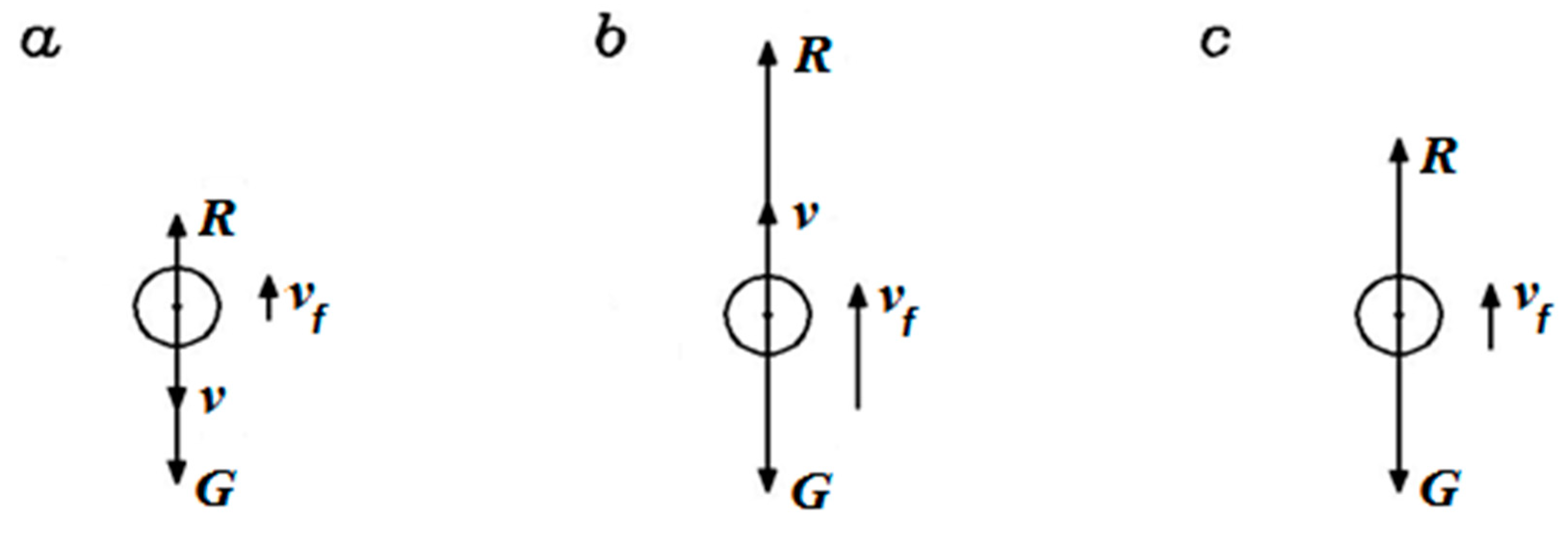
• For a vertical stream (β = 0):
  • θ_eq = π/2, for v_f > v_c;
  • θ_eq = 0, for v_f = v_c;
  • θ_eq = −π/2, for v_f < v_c.
• For a horizontal stream (β = π/2): θ_eq = arctan(−v_c/v_f);
• For a tilted stream (0 < β < π/2): θ_eq = arctan[(v_f cosθ − v_c)/(v_f sinβ)].

The particle in equilibrium continues its motion, but at a constant velocity along a straight line in the direction tilted at angle θeq. The equations of the trajectory then take the following form:

x = x₀ + v_eq cosθ_eq t

(45)

y = y₀ + v_eq cosθ_eq t

(46)

where v_eq is the absolute velocity of the particle upon reaching the equilibrium state (m/s) and x₀, y₀ are the coordinates of the particle’s location upon reaching equilibrium (m).

The absolute speed of the stable motion is equal to

v_eq = (v_f² + v_c² − 2v_fv_c cosβ)^1/2

(47)

To calculate the coordinates of the particle’s location at the initial moment of stable motion, it is necessary to solve Equations (37) and (38) by integrating the resulting functions over the entire range of [α, θ_eq].

To solve the trajectory for a particle in a stream of air, one should begin by discerning the hodograph function of the velocity in respect to θ. For that, it is necessary to solve Equation (24) with the initial conditions θ = α and v = v₀. This problem may be presented in the following form:

dv/dθ = v {v_c² sinθ + [v − v_f sin(θ + β)][v_f² + v² − 2v_fvsin(θ + β)]^1/2}/
{v_c² cosθ − v_f cos(θ + β)][v_f² + v² − 2v_fvsin(θ + β)]^1/2}
v = v(θ), v(α) = v₀, α ≤ θ ≤ θ_eq

(48)

Due to necessity of using numerical (discrete) methods, the solution to the above problem bears the form of column vectors:

θ = [θ₁, θ₂ … θ_i … θ_n]^T

(49)

v = [v₁, v₂ … v_i … v_n]^T

(50)

where every ith element of the vector θ is matched by the ith element of the v vector.

3. Results

3.1. Numerical Calculations

The numerical calculations necessary for solving the equations of motion were performed at the Academic Computer Centre CYFRONET AGH with the MATLAB packet, using a Prometheus high-performance computer. On the basis of the Runge–Kutta and NDFs methods as applied by ode45 and ode15 solvers, a hodograph function was created. This function served to test the correctness of the solutions to Equation (48) for differing entry parameters. Knowing the absolute velocity of a particle upon achieving equilibrium (described by Equation (47)) is immensely helpful for this purpose. Although in many cases a correct solution was reached, nevertheless, some problems were encountered. The most important of them are as follows:

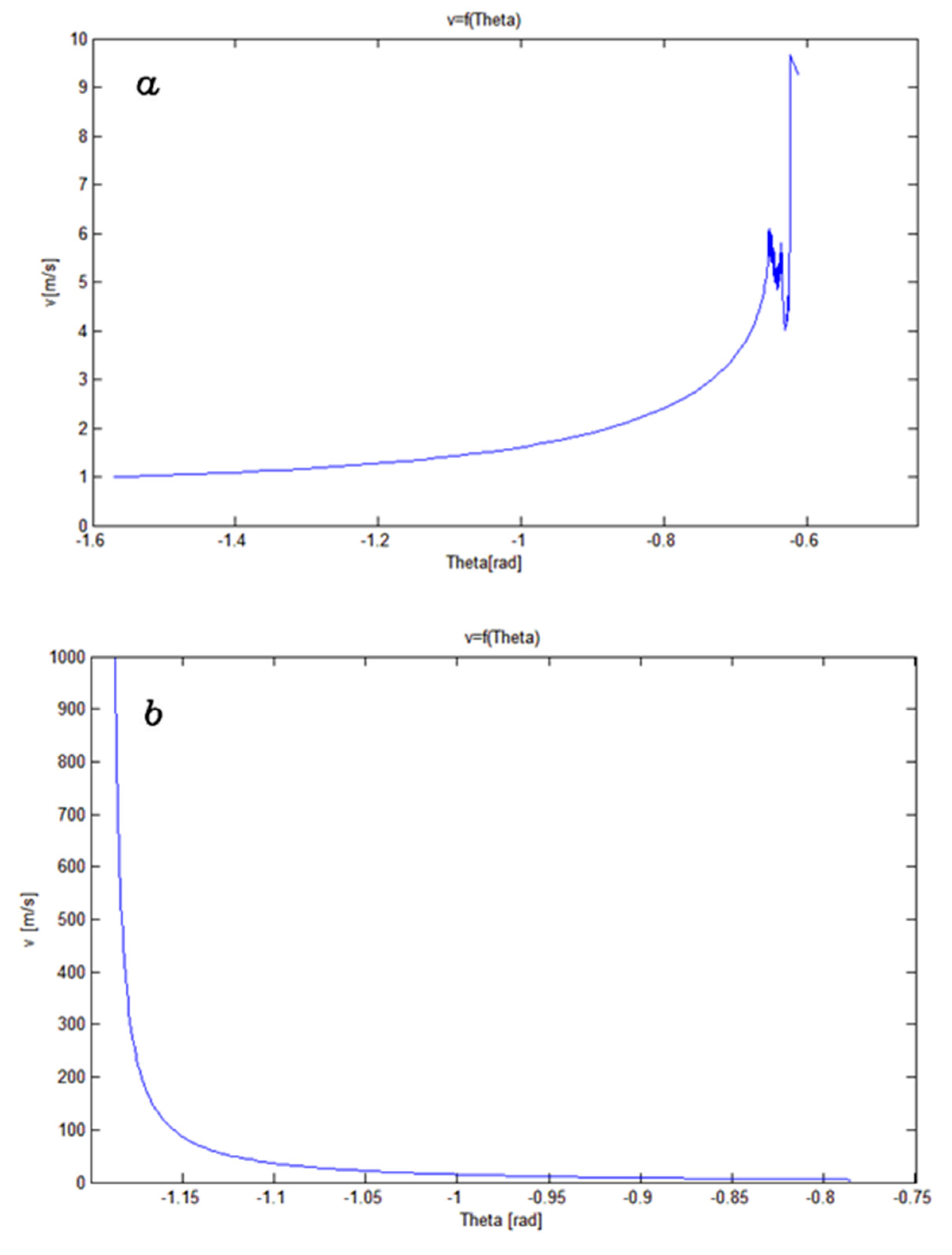
• The loss of absolute stability of a solution before reaching the boundary angle θ (Figure 5a). This problem appears when very small increases of the angle θ are accompanied by comparatively large changes in the value of the function v(θ). Bjorck and Dahlquist [28] called this problem “stiff.” It is then advisable to use methods dedicated to stiff problems. An attempt at using one, the multi-step NDFs method as realized by solverode15s, ended in failure. The algorithm for the NDFs method ends where oscillations previously began. The impossibility to reduce the length of the integration step appears to be the cause of the problem. Similar behavior characterizes other algorithms intended to solve stiff systems. Therefore, there may be a cause beyond stiffness for the observed difficulties.
• Divergence of the solution toward infinity (Figure 5b). This problem appears more illogical than the last. The velocity of the particle presented in Figure 5b grows exponentially to 10¹⁴ m/s instead of drawing toward 0.5 m/s at the boundary angle θ (as would result from Equation (47)).
• The impossibility of solving problems where the initial value of the angle θ equals its final value (i.e., particles are introduced into the stream at an angle equal to the boundary angle). For obvious reasons, Equation (24) has only a single point as a solution, which is also a known initial point. This problem concerns, for example, the horizontal introduction of a particle into a vertical stream of a velocity equal to the terminal velocity (when α = θ_eq = 0).

To find the cause of these difficulties, an analysis of the runs of various hodograph functions was performed, with the ultimate intent being to provide an approximate prediction of the run of a hodograph function in the cases of incorrect solutions.

In the first of the specified problems, the prediction used hodograph functions for particles of terminal velocity v_c = 7 m/s, introduced into the horizontal angle of velocity v_f = 10 m/s at an angle α = −π/2 and at various values of the initial velocity v₀. From the graph in Figure 6, it is easy to notice how runs of the function v(θ) met in their final part. It can be surmised that the incomplete run of the function for v₀ = 1 m/s would also meet with the others. However, for that to be possible, a single value of the angle θ must be matched with more than one value of the velocity, which contradicts the definition of a function. This would explain the incorrectness of the solution in this case.

An analysis of the remaining two problems showed the same cause of faulty solutions and could be explained in terms of the physical laws governing the motion of the particle. While the net tangential force acting on a particle causes a change in the value of velocity vector, the net normal force changes its direction and, therefore, the tilt of the tangent. As a result, the correct solution to Equation (48) may be achieved only when the net normal force maintains a constant direction during unsteady motion. The specified problems show this is not always so.

To account for that, a universal method based on swapping the variables in cases of the net normal force changing direction was proposed. In formal terms, this may be presented as

dθ/dv = (1/v) {v_c² cosθ − v_f cos(θ + β)][v_f² + v² − 2v_fvsin(θ + β)]^1/2}/
{v_c² sinθ + [v − v_f sin(θ + β)][v_f² + v² − 2v_fvsin(θ + β)]^1/2}
θ = θ(v), θ(v₀) = α, v₀ ≤ v ≤ v_eq

(51)

where v_c, v_f, v₀, α, and β are constants.

The selection of the problem to use for the hodograph function is based on the direction of the centripetal force at the initial point of motion. If it causes a change of the tangent’s tilt according to the direction of integration (from α to θ_eq), then Equation (48) is to be chosen. In the opposite case, it should be Equation (51). In practice, finding out the direction of the net centripetal force consists of finding out its sign by calculating the following expression:

sgn {cosθ − [v_f cos(θ + β) (v_f² + v² − 2v_fvsin(θ + β))^1/2]/v_c²}

(52)

After performing numerical integration, it is necessary to check if the equilibrium state was reached. Therefore, one has to compare the end values of the numerical solution with the boundary values of the angle θ and the particle velocity v. As numerical methods are always embarked with a certain error, and achieving an exact solution is practically impossible (among other reasons, due to the limited precision of machine calculation), a degree of error must be allowed. On the basis of many trial runs, the degree of error accepted was 0.01 m/s for the velocity and 0.01 rad for the angle of the tilt of the trajectory tangent.

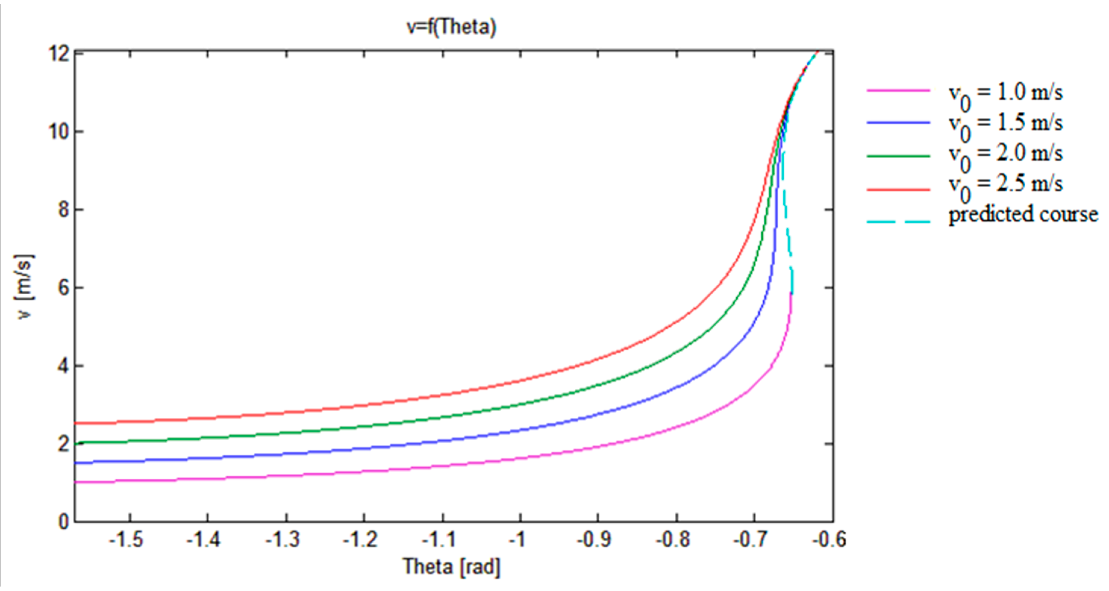
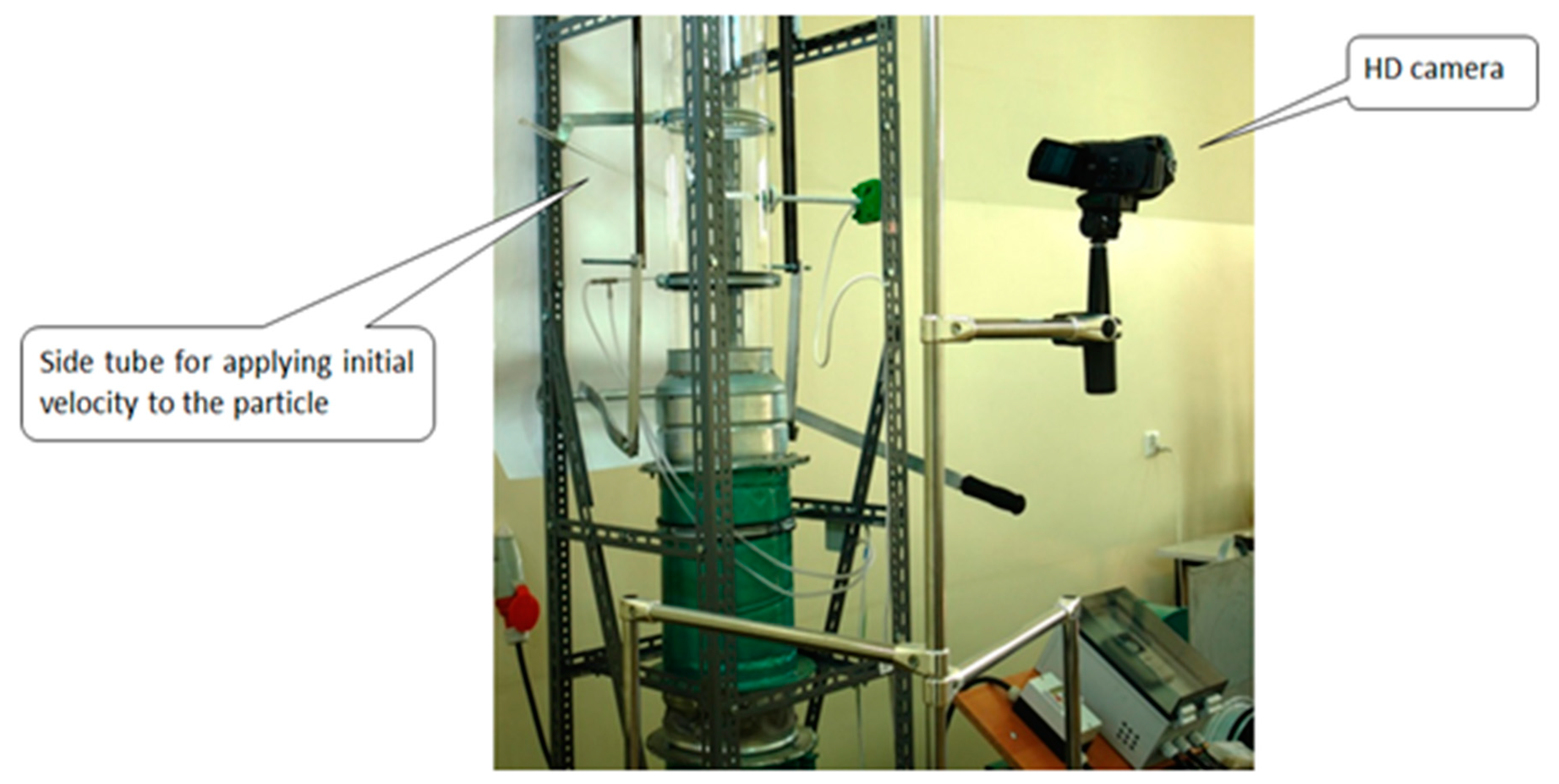
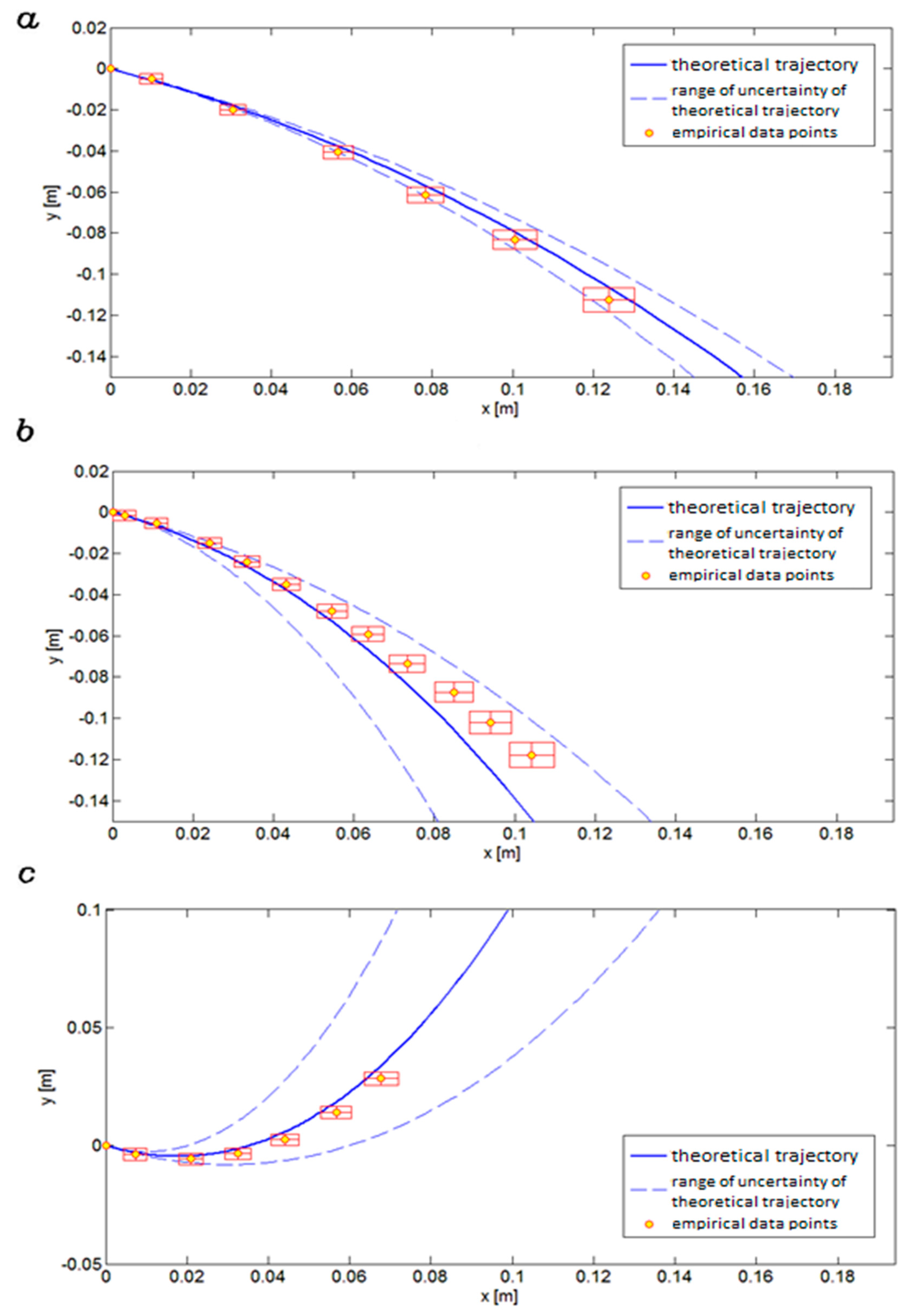
3.2. Model Verification

In order to verify the model empirically, an experimental setup was constructed on the basis of the concept by Frączek and Reguła [25]. The device consisted of a vertical aerodynamic tunnel with the air flowing from below through a set of sieves, allowing us to measure the air velocity and observe the sample at any point of the test stage cross-section, with the turbulent (Re > 8000) flow not influenced by the presence of tunnel walls. The air velocity could be adjusted in range of 0.7–20 m/s. The device was controlled through a DT9818 control module coupled with a computer and a panel coded in the LabVIEW programming language. The model is presented in Figure 7.

At first, a measurement of the terminal velocity was performed. For this purpose, grains of Schwabenkorn spelt (sized over 2 mm) were used, as they provided a relatively well-defined testing sample among available agricultural or waste materials. Their terminal velocity was measured in 100 takes with an accuracy of 0.3 m/s.

A high-resolution camera and an additional side channel to provide the particle with a given initial velocity served to register the trajectories of particles falling into the air stream (Figure 8). The air velocity in the test chamber was measured with a hot wire anemometer over 60 s at a sampling frequency of 100 Hz.

The model testing proper was performed by using a camera with a 1920 × 1080 px resolution and 60 fps registering speed to register the trajectories of particles introduced into the stream. Frames from the recording were separated by Sony Vegas Pro 8 software and subsequently analyzed in an AutoCAD 2011 packet, in order to measure the distance passed by the particle between two neighboring frames. On this basis, the initial velocity and angle in respect to air stream were calculated (Figure 9).

The accuracy of these measurements depended on the parameter in question:

• The angle α was measured using an electronic goniometer with an accuracy of 0.1°;
• The air velocity was measured with an EE65-VB5-D02 air velocity transmitter with an accuracy of ± (0.3 + 3%);
• The initial velocity of the particle v₀ was assessed by computer-assisted image analysis, tracing the path of the particle within a side vessel over a given time Δt (±0.0002 s). This resulted in the value of path length uncertainty Δs = 0.002 m. Thus, the uncertainty of the initial velocity v₀ was calculated on this basis, using the exact differentiation formula:

Δv₀ = |1/t|Δs + |−s/t²|Δt

(53)

Due to the method of calculation of the coordinates of the trajectory points, they were also burdened with measurement uncertainties, chiefly the result of the parallax error resulting from the optical effects involved in the passing of the light through the tube walls and the relative location of the camera, scaling errors, and the inaccuracies in tracing the edge of the particle on an image (Δx ≈ 2 mm). The standard uncertainties were calculated from these, providing uncertainty rectangles for each of the trajectory points (Figure 10). The calculated uncertainty values were as follows:

• For x: ±(0.0023 + 0.001%);
• For y: ±(0.0067 + 0.001%).

The theoretical trajectories were calculated according to the model’s predictions. As the arguments of the trajectory function were burdened with empirically-derived uncertainties, the theoretical trajectory was nested within an uncertainty range. The standard uncertainties of every argument of the trajectory function were calculated to find out the bounds of this range and, subsequently, trajectories were calculated for the extreme values. Thus, the calculated trajectories were then compared to the experimental values. The results of this comparison are presented in Figure 10. On the basis of this comparison, the model was verified to produce results within the uncertainty range of the empirical trajectories. In each case, this condition was fulfilled; therefore, there were no grounds to falsify the proposed model.

4. Discussion

Separation of particulate plant material in a stream of air is one of the primary material processing techniques, employed, for example, during post-harvest wheat processing, where up to 70% of impurities are removed on the basis of the aerodynamic properties of constituent particles. This creates the necessity for a study of the process of pneumatic separation, which will provide the optimal parameters for its realization. The efficiency of this process depends, among other things, on precise assessment of the optimal size of separation chambers, air velocity values, and the velocity and initial angle of the introduction of material into the stream.

As was stated in the introduction to this paper, in the majority of cases, the state of the research involves exploratory studies of specific separators. This indeed allows for the increase of separation efficiency and the lowering of energy consumption, as shown in papers by Nesterenko et al. [16], who provided quantitative data on the operation of a prototype separator, and Tobias et al. [17], who designed and tested a two-stage system for removing waste from a crop of sorghum, allowing for removal of up to 56% of leaves in a single take at the pneumatic stage. Still, their papers exhibit a similar lack of possibility of broader application. More theoretically minded exploratory studies by Panasiewicz et al. [9], who focused their attention on several cultivars of lupin, and Badretdinov et al. [18], who provided both a description of the general circulation model and a visualization of velocity trajectories, have likewise failed to account for one or more crucial aspects of modeling particle separation and movement. As described in the introduction, Badretdinov’s lack of accounting for the angle of introduction of the material into the stream was amended by Stepanenko and Kotov [19], who illustrated their results with a graph of the trajectories for three values of air velocity (7.3 m/s, 9 m/s, and 11 m/s). However, despite the similarity of these velocities to the ones used in this paper, the results can unfortunately not be compared. As stated in the introduction, the paper by Stepanenko and Kotov also delivers neither the solutions to the provided equations, nor any experimental verification.

The examples provided above reveal that the state of the research is clearly dominated by purely applied studies, usually involving the operation of specific devices. It is thus difficult to relate the results provided by any given researcher to those of others. The model presented in this paper is the first to fully account for the case of a particle introduced into the air stream at an oblique angle.

5. Conclusions

The theoretical analysis presented within this paper allowed us to create a simplified model to describe the basic parameters of the unsteady motion of particles in a stream of air, producing equations of motion solvable by numerical methods. However, for these algorithms to function, it is necessary to introduce the additional control element as in many cases, one argument is matched with two possible values. After having taken this into account, the solutions bore an acceptable level of correctness, making prediction of the approximate trajectories of solid particles in a rectilinear stream of air possible. This outcome is significant for the design of devices used for pneumatic transport and separation.

This, together with the presented method for solving equations of motion, forms a solid entry point for further development of the model, especially by expanding it to include the phenomena which have, so far, been omitted. One of the possibilities is to turn values assumed to be constant (e.g., terminal velocity, which is dependent on Reynolds number, or air velocity, which is non-uniform under real operating conditions) back into variables. The uncertainties which accompany the calculation of model parameters and the measurement of trajectory coordinates make it impossible to directly observe the influence of omitted factors. Therefore, future tests of the proposed model should be performed by more accurate methods (e.g., by using more accurate measurement devices).

Particular attention should be given to the methods of assessment of the parameters that characterize the particle. The currently dominant method of measuring the terminal velocity (by finding the equilibrium between gravity and drag) is burdened with large uncertainties, resulting from the instability of the equilibrium due to quickly changing fluctuations of air velocity and dynamic changes in the projected area, in respect to the direction of air flow.

The research described in this paper allowed us to formulate the following conclusions:

• The trajectory of particles in unsteady motion in a stream of air can be described with parametric equations of the following form:

  x = ∫^θ_α (f²(θ)cosθ/g) {(v_f/v_c²) cos(θ + β) [v_f² + f²(θ) − 2v_fvsin(θ + β)f(θ)]^1/2 − cosθ}⁻¹ dθ

  y = ∫^θ_α (f²(θ)sinθ/g) {(v_f/v_c²) cos(θ + β) [v_f² + f²(θ) − 2v_fvsin(θ + β)f(θ)]^1/2 − cosθ}⁻¹ dθ

  where f(θ) is the absolute particle velocity hodograph function, equal to the solution of the following differential equation:

  dv/dθ = v {v_c² sinθ + [v − v_f sin(θ + β)][v_f² + v² − 2v_fvsin(θ + β)]^1/2}/
  {v_c² cosθ − v_f cos(θ + β)][v_f² + v² − 2v_fvsin(θ + β)]^1/2}
• To solve the proposed equations of motion, it is necessary to use numerical methods for solving differential equations and integration with additional control over the possible matching of several hodograph function values to a single argument.

References

1. Klinzing, G.E. A review of pneumatic conveying status, advances and projections. Powder Technol. 2018, 333, 78–90. [Google Scholar] [CrossRef]
2. Lourenço, G.A.; Gomes, T.L.C.; Duarte, C.R.; Ataíde, C.H. Experimental study of efficiency in pneumatic conveying system’s feeding rate. Powder Technol. 2019, 343, 262–269. [Google Scholar] [CrossRef]
3. Zheng, K.; Du, C.; Li, J.; Qiu, B.; Yang, D. Underground pneumatic separation of coal and gangue with large size (≥50 mm) in green mining based on the machine vision system. Powder Technol. 2015, 278, 223–233. [Google Scholar] [CrossRef]
4. Bi, H.; Zhu, H.; Zu, L.; He, S.; Gao, Y.; Gao, S. Pneumatic separation and recycling of anode and cathode materials from spent lithium iron phosphate batteries. Waste Manag. Res. 2019, 37, 374–385. [Google Scholar] [CrossRef] [PubMed]
5. Grandison, A.S.; Lewis, M.J. (Eds.) Separation Process in the Food and Biotechnology Industries; Woodhead Publishing: Cambridge, UK, 1996. [Google Scholar]
6. Innocentini, M.D.M.; Barizan, W.S.; Alves, M.N.O.; Pisani, R., Jr. Pneumatic separation of hulls and meats from cracked soybeans. Food Bioprod. Process. 2009, 87, 237–246. [Google Scholar] [CrossRef]
7. Güner, M. Pneumatic conveying characteristics of some agricultural seeds. J. Food Eng. 2007, 80, 904–913. [Google Scholar] [CrossRef]
8. Panasiewicz, M. Analysis of the pneumatic separation process of agricultural materials. Int. Agrophys. 1999, 13, 233–239. [Google Scholar]
9. Panasiewicz, M.; Sobczak, P.; Mazur, J.; Zawiślak, K.; Andrejko, D. The technique and analysis of the process of separation and cleaning grain materials. J. Food Eng. 2012, 109, 603–608. [Google Scholar] [CrossRef]
10. Anantharaman, A.; Cahyadi, A.; Hadinoto, K.; Chew, J.W. Impact of particle diameter, density and sphericity on minimum pickup velocity of binary mixtures in gas-solid pneumatic conveying. Powder Technol. 2016, 297, 311–319. [Google Scholar] [CrossRef]
11. Markowski, M.; Żuk-Gołaszewska, K.; Kwiatkowski, D. Influence of variety on selected physical and mechanical properties of wheat. Ind. Crop. Prod. 2013, 47, 113–117. [Google Scholar] [CrossRef]
12. Łukaszuk, J.; Molenda, M.; Horabik, J.; Szot, B.; Montross, M.D. Airflow resistance of wheat bedding as influenced by the filling method. Res. Agric. Eng. 2008, 54, 50–57. [Google Scholar] [CrossRef] [Green Version]
13. Komarnicki, P.; Banasiak, J.; Bieniek, J. Rozkład aerodynamicznych parametrów stanu równowagi procesowej czyszczenia ziarna. Inż. Rol. 2008, 4, 389–396. [Google Scholar]
14. Klinzing, G.E.; Basha, O.M. A correlation for particle velocities in pneumatic conveying. Powder Technol. 2017, 310, 201–204. [Google Scholar] [CrossRef]
15. Sun, S.; Yuan, Z.; Peng, Z.; Moghtaderi, B.; Doroodchi, E. Computational investigation of particle flow characteristics in pressurised dense phase pneumatic conveying systems. Powder Technol. 2018, 329, 241–251. [Google Scholar] [CrossRef]
16. Nesterenko, A.V.; Leshchenko, S.M.; Vasylkovskyi, O.M.; Petrenko, D.I. Analytical assessment of the pneumatic separation quality in the process of grain multilayer feeding. INMATEH Agric. Eng. 2017, 53, 65–70. [Google Scholar]
17. Tobias, E.; Gaudet, C.; Viator, H.; Aragon, D.; Ehrenhauser, F. Leaf and panicle separator for sweet sorghum. Sugar Tech. 2018, 20, 252–260. [Google Scholar] [CrossRef]
18. Badretdinov, I.; Mudarisov, S.; Tuktarov, M.; Arslanbekova, S. Mathematical modeling of the grain material separation in the pneumatic system of the grain-cleaning machine. J. Appl. Eng. Sci. 2019, 641, 529–534. [Google Scholar] [CrossRef]
19. Stepanenko, S.P.; Kotov, B.I. Pneumonitis fractionation of grain materials in air streams of variable structure. Mach. Energ. J. Rural Prod. Res. 2020, 11, 127–132. [Google Scholar]
20. Kryszak, D.; Bartoszewicz, A.; Szufa, S.; Piersa, P.; Obraniak, A.; Olejnik, T.P. Modeling of transport of loose products with the use of the non-grid method of discrete elements (DEM). Processes 2020, 8, 1489. [Google Scholar] [CrossRef]
21. Lift, R.; Grace, J.R.; Weber, M.E. Bubbles, Drops and Particles; Academic Press: New York, NY, USA, 1978. [Google Scholar]
22. Orzechowski, Z. Przepływy Dwufazowe, Jednowymiarowe, Ustalone, Adiabatyczne; PWN: Warszawa, Poland, 1990. [Google Scholar]
23. Orzechowski, Z.; Prywer, J.; Zarzycki, R. Mechanika Płynów w Inżynierii i Ochronie Środowiska; WNT: Warszawa, Poland, 2008. [Google Scholar]
24. Mohsenin, N.N. Physical Properties of Plant and Animal Materials; Gordon and Breach Science Public: New York, NY, USA, 1986. [Google Scholar]
25. Frączek, J.; Reguła, T. Metodyczne aspekty pomiaru właściwości aerodynamicznych cząstek stałych pochodzenia roślinnego. Acta Agrophys. 2012, 19, 515–525. [Google Scholar]
26. Grochowicz, J. Machines for Cleaning and Sorting of Seeds; PWRiL: Warsaw, Poland, 1980. [Google Scholar]
27. Frączek, J.; Wróbel, M. Metodyczne aspekty oceny kształtu nasion. Inż. Rol. 2006, 87, 155–163. [Google Scholar]
28. Dahlquist, G.; Bjorck, A. Numerical Methods in Scientific Computing; SIAM: Philadelphia, PA, USA, 2008; Volume 1. [Google Scholar]
Figure 1. Forces acting on a particle in a vertical stream of air. (a) G > R; (b) G < R; and (c) G = R. The velocity of the fluid stream is denoted as vf.
Processes 09 00005 g001
Figure 2. A particle in a stream of fluid shown in (a) a force diagram and (b) a velocity diagram. The dashed line denotes the particle trajectory. The dashed and dotted line is the direction of the fluid current.
Processes 09 00005 g002
Figure 3. Influence of various factors on aerodynamic properties.
Processes 09 00005 g003
Figure 4. Movement of a particle in a vertical stream of air, displaying (a) particle trajectory and (b) the vector components of forces and velocities. The dashed line denotes the particle trajectory.
Processes 09 00005 g004
Figure 5. Incorrect solutions to the problem. (a) A loss of solution stability for v0 = 1.0 m/s, α = −45°, vc = 7.0 m/s, vf = 10.0 m/s, β = 90°; and (b) runoff of the solution toward infinity for v0 = 5.0 m/s, α = −45°, vc = 10.5 m/s, vf = 10.0 m/s, β = 0°.
Processes 09 00005 g005
Figure 6. A prediction of the run of a velocity hodograph function for incorrect solutions.
Processes 09 00005 g006
Figure 7. Concept drawing of the experimental setup for the measurement of the aerodynamic properties of plant material, showing (a) the general view, (b) the flow homogenization section, and (c) the particle introduction method. 1 = duct fan, 2 = throttle, 3 = amortizing spigot, 4 = homogenization section, 5 = acryl pipe, 6 = camera, 7 = honeycomb structure, 8 = sieve screens, 9 = lever, 10 = sieve, 11 = connector, 12 = holder, and 13 = guide bar [18]. Image provided with permission from Tomasz Reguła (source: own work).
Processes 09 00005 g007
Figure 8. The setup for the measurement of the aerodynamic properties of solid particles.
Processes 09 00005 g008
Figure 9. The outline of the trajectory and the method of conducting the measurements on the basis of the registered video stream.
Processes 09 00005 g009
Figure 10. Theoretical and empirical trajectory of the particle (α = −27°) at (a) vf = 2.7 m/s, v0 = 1.4 m/s; (b) vf = 6.2 m/s, v0 = 0.6 m/s; and (c) vf = 12.8 m/s, v0 = 0.8 m/s.
Processes 09 00005 g010
Publisher’s Note: MDPI stays neutral with regard to jurisdictional claims in published maps and institutional affiliations.