Combined Response Surface Method and Modified Differential Evolution for Parameter Optimization of Friction Stir Welding

Abstract

In this study, we constructed a new algorithm to determine the optimal parameters for friction stir welding including rotational speed, welding speed, axial force, tool pin profile, and tool material. The objective of welding is to maximize the ultimate tensile strength of the welded aluminum. The proposed method combines the response surface method and the modified differential evolution algorithm (RSM-MDE). RSM-MDE is a method that involves both experimental and simulation procedures. It is composed of four steps: (1) finding the number of parameters and their levels that affect the efficiency of the friction stir welding, (2) using RSM to formulate the regression model, (3) using the MDE algorithm to find the optimal parameter of the regression model obtained from (2), and (4) verifying the results obtained from step (3). The optimal parameters generated by the RSM-MDE method were a rotation speed of 1417.68 rpm, a welding speed of 60.21 mm/min, an axial force of 8.44 kN, a hexagon-tapered tool pin profile, and the SKD 11 tool material. The ultimate tensile strength obtained from this set of parameters was 294.84 MPa, which was better than that of the RSM by 1.48%.

1. Introduction

Aluminum is widely used to produce products in many industries, such as the automotive, shipyard, aviation, and electric train industries, due to its high strength, light weight, high toughness, resistance to breakage, good corrosion resistance, and ability to reduce product damage without decreasing product quality [1]. Producing large sheets of aluminum can be expensive and sometimes impossible using the current machine technology. Welding methods are often used to join small sheets of aluminum into bigger parts to produce the part needed. Welding is a process in which metals are joined using high heat to melt parts together, and the metal is then allowed to cool to normal temperature. Numerous welding methods exist, including gas metal arc welding using metal inert gas or tungsten inert gas, arc welding, gas welding, spot welding [2,3], and friction stir welding (FSW).

FSW is one of the most popular welding methods used to join two sheets of aluminum. FSW can be used to weld a variety of aluminum alloys [4]. FSW can create high-quality welded areas compared to other conventional welding processes, and it can be used to join metal and non-metal materials [5]. FSW is a solid-state welding (SSW) process invented by the British Welding Institute [6]. This technique attaches metals together at a temperature lower than the melting temperature of the cast based on the heat from friction where the shoulders touch the sheet and rotate at a specified welding speed along with pressure. FSW is widely used to produce parts [7] for airplanes, boats, trucks, pipeline work, electrical work, electronics, furniture, vacuum cleaner suction pipes, and rail fines. Usually, the parameters that influence FSW include tensile strength, hardness, wear, and corrosion, rotational speed, welding speed, axial force, tool pin profile, pin diameter, and tool pin material [8,9,10].

One of the important characteristics of FSW is to obtain welded aluminum that has the highest ultimate tensile strength (UTS). The ultimate tensile strength (UTS) is the maximum stress that a material can tolerate while being pulled before breaking. In brittle materials, the UTS is close to the yield point, whereas, for ductile materials, the UTS can be higher. The UTS is normally investigated by executing a tensile test in a tensile testing machine. In this study, we used the testing machine model CY-6040A1, c.b.n. testing corporation Co. Ltd., Bangkoknoi, Bangkok, Thailand.

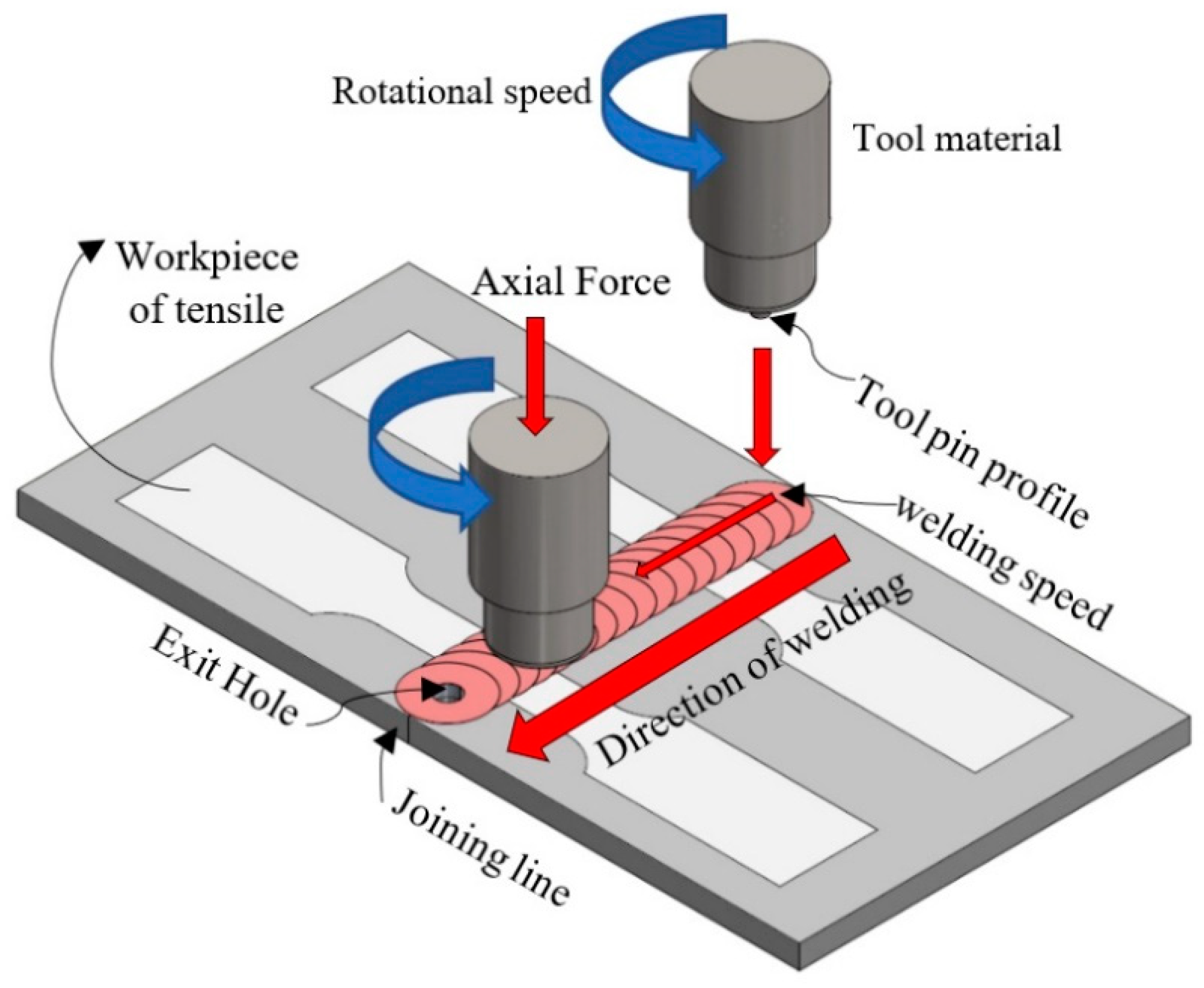
From the literature review, we found that two group of parameters affect the UTS of FSW. The first group includes three parameters: (1) rotation speed, (2) welding speed, and (3) axial force. In this group, the parameter values are real numbers, such as a rotation speed of 800 rpm. The second group is defined as the categorized parameters. In this group, the two types of parameters are (1) tool pin profile and (2) tool pin material. Details of all five parameters are shown in Figure 1.

The integrity of friction stir welding depends on the proper setting of welding parameters. FSW process parameters affect the heat of perfect welds. Welding heat depends on the setting of parameters such as rotation speed, welding speed, and the axial force of the tool pin profile. When the tool pin profile rotates at a constant speed and is pressed against the workpiece surface, friction causes heat in the welding process due to mechanical force. The heat increases to the extent that the materials soften and, at an appropriate level, the materials can be welded together.

In welding, welding speed is a parameter to control the amount of heat in the area in which the tool pin profile passes. If the welding speed is too high, the heat level in the joint’s weld zone will be too low, resulting in incomplete bonding of the material. Conversely, if the welding speed is too slow, excess heat will accumulate in the material, affecting structural change defects in the weld. Therefore, the amount of heat during welding depends on controlling the process parameters; the generation of too much or too little heat will affect the structural differences in the welding zone and may cause defects [11]. The relationship between the parameters mentioned for the determination of the weld heat can be calculated from Equation (1) [12].

$$Q_{slide}=\frac{2}{3}\pi \mu p\varpi \left[{\left(\frac{D}{2}\right)}^3-{\left(\frac{d}{2}\right)}^3\right]\left(1+tan\alpha \right),$$

(1)

where Q_slide is the generated heat while sliding (watts), μ is the friction coefficient of the material, p is the axial force (kN), ϖ is the tool angular rotation speed (rad⁻¹), D is the diameter of the shoulder (mm), d is the diameter of the pin (mm), and α is the shoulder angle (°).

Table 1. Suggested parameters and their values gathered from the literature.

Author	Rotational Speed (rpm)	Welding Speed (mm/min)	Axial Force (kN)	Materials
Elatharasan and Kumar (2013)	800, 1000, and 1200	30, 60, and 90	6, 8, and 10	AA6061
Ravi Sankar and Umamaheswarrao (2017)	800–1400	30–55	6	AA6061
Salehi et al. (2012)	800–1600	40–160	-	AA6061
Elanchezhian et al. (2014)	1200, 1300, and 1400	75, 100, and 125	5, 6, and 7	AA8011–AA6062
Chanakyan et al. (2020)	900, 1100, and 1300	33, 45.5, and 58	4, 5, and 6	AA6082
Muthu Krishnan et al. (2018)	800–1300	20–40	3–8	AA6063 and A319
Prasad and Kumar Namala (2018)	800, 1200, and 1600	20, 50, and 80	-	AA5083–AA6061
Rajakumar et al. (2011)	862–1337	60–127.5	6–10.37	AA6061
Elangovan et al. (2009)	800–1600	15–135	5–9	AA6061

lists the welding parameters and their values gathered from the literature review [8,9,13,14,15,16,17,18,19]. The table shows that three factors affect the tensile efficiency: rotational speed (rpm), welding speed (mm/min), and axial force (kN).

Other factors that affect the UTS of FSW that are not in the literature (Table 1) are the tool material and tool pin profile. Bringas [20] and Banik et al. [21] recommended the use of two types of tool materials (SKD 11 and ST 42), and they included three types of tool pin profiles (cylindrical tapered (CT), square tapered (ST), and hexagon tapered (HT)) with FSW. The chemical compositions of SKD 11 and ST 42 are shown in

Table 2. Chemical compositions of tool materials.

	Chemical Composition
	C	Si	Mn	P	S	V	Mo	Cr	Fe
SKD 11	1.60	0.40	0.60	0.30	0.03	0.50	1.20	13.0	81.9–86.6%
ST 42	0.21	0.40	1.35	0.04	0.05	0.15	-	-	98%

.

ST 42 is made of low-carbon steel and SKD 11 is made of high-carbon steel. Both types of tools use the quenching method to improve the mechanical properties. The target hardness of the tools must be greater than 500 HB (Brinell hardness test). ST 42 and SKD 11 have melting points of 1421–1460 °C, which are greater than the melting point of the base material (AA6061-T6 Nissin part Co. Ltd., Nonthaburi, Thailand) used in this research (AA6061-T6 has a melting point of 652 °C and hardness of 90 HB). The wear rate of the tool is low due to the huge difference in hardness and melting point of the tool pin and base material. Therefore, the selection of an appropriate tool pin and base material can increase the life of the tool. Each tool pin has a shoulder diameter of 18 mm, pin length of 6 mm, and pin angle of 6°. The tool pin profile length should be shorter than the thickness of the pin of the base material (AA6061-T6) in order to properly insert the pin profile into the base material [22]. During welding, the tool pin profile is inserted into the material to create the heat generated from friction. Simultaneously, the base material becomes soft and deforms. In the state of plastic deformation, the material becomes homogeneous and a weld bond occurs; therefore, the material is unable to penetrate through the lower surface of the workpiece. At the beginning of the welding process, the tool pin profile is firmly pressed and inserted into the material until the shoulder of the tool pin profile contacts the workpiece surface due to axial force. As a result, friction occurs between the shoulder of the tool pin profile and the workpiece. The material rapidly heats up because of the friction between the tool pin profile and the surface of the workpiece. This causes the material to soften and deform around the welding zone. Because of the appropriate heat transfer capability of the AA6061-T6, the heat around the tool pin profile that penetrates the material spreads more easily. The material softens into the mixture, resulting in a welding line. The tool materials for each of the pin profiles are shown in Figure 2a–c.

In this study, five parameters ((1) rotation speed, (2) welding speed. (3) axial force, (4) tool pin profile, and (5) tool pin material) were analyzed to determine the optimal values or types of all parameters. These five parameters were not previously simultaneously studied for FSW in the literature.

One of the most popular methods used to determine the optimal welding parameters is the response surface method (RSM) [23,24]. To find the optimal value of parameters, RSM is firstly used to design the experiment and formulate the second-order mathematical model, sometimes called quadratic programming (QP). Then, the Minitab optimizer or optimization software such as excel solver, Lingo, and Lindo is used to find the optimal value of parameters. In optimization software, exact methods such as the simplex method, dual simplex method, branch and bound method, and generalized reduced gradient (GRG) are used as the optimization method. Even though the exact method can guarantee the optimal solution, when the size of the problem is growing, the exact method is not applicable to solve non-deterministic polynomial-time hardness (NP-hard) problems within a reasonable time [25,26,27].

The mathematical model obtained from the RSM method is a type of quadratic programming (QP) which is proven to be an NP-hard problem [28]. To avoid the time-consuming process of solving the QP using exact methods, heuristics such as those developed by Achterberg and Berthold [29], and Glover and Lodi [30], and metaheuristic methods like simulated annealing [31], as well as evolutionary and memetic algorithms [32,33], are applied to solve QP. Such heuristics are often quite effective, and they can be implemented on very modest computational hardware, even without any theoretical guarantees, to find the optimal solution. However, the heuristic and metaheuristic methods may provide a sufficiently good solution to a complex problem in a reasonable amount of time. This is the first reason why we need to design the heuristic method to optimize the model obtained from Minitab software instead of using optimization software.

Another reason that a heuristic method is needed in our research is that we were interested in discovering the value/type of five parameters. Two of these parameters are categorical parameters (three types of tool pin profile and two types of tool material). These two parameters will force the RSM to generate six regression models, which prevents solving all given models at once using optimization software such as excel solver and Lingo. All six models will be solved one by one. The best model among all six models will be the representative solution of the methods. This makes it inconvenient to use the solver to solve QP. To avoid this inconvenience, we design a heuristic method that can solve all models generated by RSM at the same time.

Currently, there is no research that applied a metaheuristic approach to determine the appropriate value of parameters in FSW. In this paper, the modified differential evolution algorithm (MDE) is used to determine the optimal values of the parameters.

Differential evolution algorithm (DE) is a novel evolutionary technique introduced by Storn and Price [34]. DE can be effectively applied for both continuous and discrete optimization problems. DE uses a simple operator, with classical operators such as crossover, mutation, and selection, to create new candidate solutions. Due to its effectiveness and simplicity, DE was used for production scheduling [35,36,37], manufacturing [38,39], production processes [40,41,42,43], and transportation [44,45,46] DE sometimes experiences problems in finding a good solution because it can easily get stuck in local optima. This problem can be avoided by restarting the algorithm, introducing a new random vector into the algorithm, and changing the neighborhood strategy to search for a new solution. In this study, we introduced a trial vector reproduction process to improve the capability of DE. This method helps the original DE to escape from the local optimum when needed. We call our new DE method the modified differential evolution (MDE) algorithm.

RSM and MDE (RSM-MDE) were combined in this study to find the optimal parameters of FSW to find the maximum UTS. The proposed method is both experiment-based and simulation-based. The experimental part (RSM) was applied to a real aluminum specimen, while the simulation part (MDE) was performed on a computer. All specimens used in the experiment were AA6061-T651 aluminum (Nissin part Co. Ltd., Nonthaburi, Thailand).

AA6061-T651 aluminum was chosen because it is widely used in the aerospace, aircraft, and automobile industries. It composes of aluminum, silicon, and magnesium (Al–Si–Mg), giving it an excellent strength-to-weight ratio, good ductility, corrosion resistance, and cracking resistance in adverse environments [47,48].

The rest of this article is organized as follows: Section 2 outlines the proposed method used to optimize the welding parameters, Section 3 describes the experimental framework, and Section 4 provides the conclusion and recommendations for future work.

2. Proposed Method: RSM-MDE

RSM-MDE was used to find the optimum values of the parameters for FSW. The RSM-MDE algorithm is illustrated in Figure 3, showing its four steps: (1) finding the number of parameters and their levels that affect the efficiency of FSW, (2) using the RSM to formulate the regression model to predict the suitable parameters of the welding, (3) using the MDE algorithm to find the optimal parameters of the regression model obtained from step (2), and (4) verifying the results obtained from step (3). The process and the results from steps (1) to (3) are described below.

2.1. Finding the Number of Parameters and Their Levels That Affect FSW Efficiency

Many different methods can be used to find parameters and their levels that affect FSW: preliminary experiments, the Delphi method, and surveying the literature. In this study, we surveyed the literature to find the number and the level of each parameter that affects the UTS.

In our experiment, we used the information in Table 1 to determine the parameters and their values. The minimum and maximum values of the parameters were set as follows: (1) rotational speed = 800 to 1600 rpm, (2) welding speed = 15 to 135 mm/min, and (3) axial force = 5 to 9 kN. We used two types of tool pin material, SKD 11 and ST 42, as suggested by Bringas et al. [20], and three types of tool pin profile (cylindrical tapered (CT), square tapered (ST), and hexagon tapered (HT)) as suggested by Banik et al. [21]. The combinations of the parameters for the experiment are detailed in Figure 4.

2.2. Using RSM to Formulate the Regression Model

The upper and lower limits of the parameters in Section 2.1 were set to 1.68 and −1.68. The intermediate coded values were calculated using Equation (2).

$$X_i=1.682\frac{\left[2X-\left(X_{\mathrm{Max}}+X_{\min }\right)\right]}{X_{\mathrm{Max}}}-X_{\min ,}$$

(2)

where $X_i$ is the required coded value of a variable X, X is any value of the variable from $X_{\min }$ to $X_{\mathrm{Max}}$, and $X_{\min }$ and $X_{\mathrm{Max}}$ are the lowest and highest predefined values of the parameter, respectively.

Table 3. Parameters in the experiment.

Continuous Variable
Parameter	Levels
	−1.682	−1	0		1	1.682
Rotational speed (rpm), S	800	960	1200		1440	1600
Welding speed (mm/min), F	15	40	110		75	135
Axial force (kN), A	5	6	7		8	9
Categorical Variables
Parameter	Levels
Tool pin profile, T	Cylindrical tapered (CT)		Square tapered (ST)		Hexagon tapered (HT)
Type of material, M	SKD 11			ST 42

provides the details of each coded and uncoded parameter, which includes the upper and lower bounds of these parameters.

Statistical software Minitab (Minitab Inc., State College, PA, USA) was used to design and create the experimental models and carry out problem analysis. The quadratic model shown in Equation (3) was expected to be obtained from the experiment.

$$y=b_0+{\displaystyle \sum }_i^k{b}_i{x}_i+{\displaystyle \sum }_i^k{b}_{ii}{x}_i^2+{\displaystyle \sum }_i{\displaystyle \sum }_j{b}_{ij}{x}_i{x}_j+\epsilon ,$$

(3)

where $y$ is the ultimate tensile strength (response), $x_i$ is the uncoded level of the variables, $\epsilon$ is the fitting error, the coefficient $b_0$ is the constant value or intercept, and coefficients $b_i$, $b_{ii},$ and $b_{ij}$ represent the linear, quadratic, and interaction terms of the variables, respectively [49].

2.3. Using the MDE Algorithm to Find the Optimal Parameters

The MDE algorithm proposed in this article has six steps: (1) generate initial solution, (2) perform mutation process, (3) perform recombination process, (4) trial vector reproduction process, (5) perform selection process, and (6) redo steps (2)–(5) until the stopping criterion is met. The use of MDE to determine the optimal FSW operating parameters to maximize UTS is explained below.

2.3.1. Generate the Initial Solution

In this step, a set of 3 × 1 vectors is randomly generated. The number of randomly generated vectors is equal to the fixed number (NP). The random value that is inserted in the positions of the vector are bounded by the upper and lower values of each parameter. Position 1 of the vector represents the rotational speed value, whereas positions 2 and 3 represent the welding speed and axial force, respectively. An example of the 10 random vectors (NP = 10) is provided in

Table 4. An example of five initial target vectors.

Factor	NP 1	NP 2	NP 3	NP 4	NP 5	NP 6	NP 7	NP 8	NP 9	NP 10
Rotational speed	1363	1097	1020	1484	1516	1269	1331	800	1171	1388
Welding speed	66	67	33	47	96	132	90	59	36	126
Axial force	9	8	9	5	6	7	8	9	5	9

.

From Table 4, if we focus on vector 1 (NP1), the values in positions 1, 2, and 3 are 1363, 66, and 9, respectively. This parameter was calculated to find the maximum UTS using the equation obtained from experimental analysis by replacing the values in the positions with variables S, F, and A.

2.3.2. Perform Mutation Process

The mutation process was performed randomly with a set of target vectors obtained from Section 2.3.1 using in Equations (4) and (5).

$$\frac{\frac{DE}{rand}}{1} V_{i,G+1}=X_{r1,G}+F\left(X_{r2,G}-X_{r3,G}\right),$$

(4)

$$\frac{\frac{\frac{DE}{best}}{best2}}{2} V_{i,G+1}=X_{best,G}+F\left(X_{r1,G}-X_{r2,G}\right)+F\left(X_{best2,G}-X_{r3,G}\right),$$

(5)

where $X_{i,G}$ is the target vector, $V_{i,G+1}$ is the mutant vector, and $X_{r1G}, X_{r2G}, \mathrm{and} X_{r3G}$ are the vectors that we randomly selected from the target vector. $X_{best,G}$ is the best vector found to date and $X_{best2,G}$ is the second best vector found to date. F is a scaling factor, which is a self-adaptive parameter, ranging from 0–2. In our experiment, F was initially set to 0.8 and was randomly changed by ±0.05 for each individual vector. The value of F of the best vector in the current iteration was set to the current F value, which was used as the base F value to be adapted by the vectors in the next iteration. An example of how to calculate a mutant vector using Equations (4) and (5) is provided in

Table 5. Example of calculating mutant vector values from NP1 formulas.

Factor/Vectors	Xr1,G	Xr2,G	Xr3,G	Xr4G	Xr5,G	DE/rand/1	DE/best/best2/2
Rotational speed	1247	830	947	1337	947	1153.4	1487
Welding speed	128	131	29	100	49	209.6	189.8
Axial force	7	7	6	5	9	7.8	7.8

.

2.3.3. Perform Recombination Process

This process generated the trial vector $(U_{i,G+1})$ using Equation (6), where CR is the self-adaptive parameter, which was first set to 0.6. We used the same method to adapt the current CR value as the method for adapting F, where ${\mathrm{rand}}_{i,j}$ is a random number.

$$U_{i,G+1}=\{\begin{array}{l}{\mathrm{V}}_{i,j,\mathrm{G}+1} \mathrm{if} {\mathrm{rand}}_{i,j} \le \mathrm{CR} \mathrm{or} j=I_{rand}\\ {\mathrm{X}}_{i,j,\mathrm{G}} \mathrm{if} {\mathrm{rand}}_{i,j} >\mathrm{CR} \mathrm{or} j=I_{rand}\end{array}$$

(6)

After the recombination process, a new process is introduced to the original DE to produce a second-order trial vector (2nd-Tr), which is generated from one of two methods: (1) vector transition process and (2) vector K-cyclic move process.

2.3.4. Trial Vector Reproduction Process

As mentioned above, this process is used after the recombination process. One of two trial vector reproduction processes is selected for use in the original DE to obtain the MDE algorithm. These two methods are the vector transition process and the K-variable process.

Vector Transition Process (VTP)

This process starts from an integer number randomly selected from 1 to D, where D is the number of positions in the vector. Let us call this number the number of transition points (NT). Then, we randomly select the NT positions within D positions. Finally, the selected positions randomly generate a new value in the position.

Table 6. Example of the vector transition process.

Original Vector
Factor	NP1	NP2	NP3	NP4	NP5
Rotational speed	1363	1097	1020	1484	1516
Welding speed	66	67	33	47	96
Axial force	9	8	9	5	6
Accompany Vector
Factor	NP1	NP2	NP3	NP4	NP5
Rotational speed	1363	1276	1020	1484	1516
Welding speed	66	67	33	45	96
Axial force	9	8	9	5	6

shows the VTP. Positions 1 of NP2 and 2 of NP4 are selected as the transition points (the pre-selected number of the transition points is 2). The values in these positions are randomly generated, while other position values remain unchanged.

Vector K-Cyclic Move Process (KCM)

The KCM includes three steps: (1) randomly select value of k (the value of k lies between 2 and NP1), (2) randomly select k vectors of each position, and (3) cyclically move the value in the positions of the selected vector according to the selection order executed in step (2).

Table 7. Example of the vector k-cyclic move process (KCM).

Original Vector
Factor	NP1	NP2	NP3	NP4	NP5
Rotational speed	1363	1097	1020	1484	1516
Welding speed	66	67	33	47	96
Axial force	9	8	9	5	6
New Trial Vector
Factor	NP1	NP2	NP3	NP4	NP5
Rotational speed	1363	1516	1020	1097	1484
Welding speed	47	66	33	67	96
Axial force	9	9	5	8	6

provides an example of the KCM. If k = 3, then we randomly select the k vector for each position. For position 1, the selected vector order is NP5, NP2, and NP4, with new values in positions NP5, NP2, and NP4 of 1484, 1516, and 1097, respectively. Then, we repeat this step until all positions of vectors are moved.

When the new trail vector is produced, it is compared with the original trial vector. The vector with a better objective function is used as the trial vector in the selection process.

2.3.5. Selection Process

This process is used to generate the target vectors for the next iteration of the simulation using Equation (7). The target vector of the next iteration is equal to the trial vector or the current target vector, depending on which vector has lower energy usage.

$$X_{i,G+1}=\{\begin{array}{c}{\mathrm{U}}_{i,j,\mathrm{G}} \mathrm{if} f ({\mathrm{U}}_{i,j,\mathrm{G}})\le f ({\mathrm{X}}_{i,j,\mathrm{G}})\\ {\mathrm{X}}_{i,j,\mathrm{G}} \mathrm{otherwise}\end{array},$$

(7)

where $X_{i,\mathrm{G}+1}$ is the target vector of the next iteration, ${\mathrm{U}}_{i,j,\mathrm{G}}$ is the trial vector of the current iteration, and ${\mathrm{X}}_{i,j,\mathrm{G}}$ is the target vector in the current iteration.

3. Experimental Framework and Results

Minitab 19 software (Minitab, LLC, State College, PA, USA) was used to calculate the result of the RSM. The DE algorithm was coded in Dev C++ (Bloodshed Software until 2005, Orwell (Johan Mes) since 2011). For all simulations and calculations, we used a personal computer (PC; Intel Core i3 central processing unit (CPU), 3.70 GHz random access memory (RAM) Double Data Rate 4 (DDR4) 8 GB, Intel, Santa Clara, CA, USA). The computational results are divided into three parts: the result from the RSM; the result for the proposed problem using RSM-MDE, which was used to compare the effectiveness of RSM-MDE with RSM; the result of the real experiment using the parameter levels determined in the second part to confirm the reliability of the theoretical levels of the parameters.

3.1. Result Using the Original Method (RSM)

We started the RSM using central composite design (CCD) to design the experiment as suggested by Bezerra et al., Candioti et al., and Politis et al. [50,51,52]. Five controlled parameters were set: rotational speed (S), welding speed (F), axial force (A), tool pin profile (T), and type of material (M). The CCD produced 120 experiments; thus, 120 specimens were prepared, as shown in Figure 5.

Details of the specimens are listed in

Table 8. Details of the tested specimens.

Material	Size (mm)	Thickness (mm)	Maximum Tensile Strength (MPa)
AA6061-T6	100 × 120	6	310

.

FSW was executed using the American Welding Society standard [53]. The welding had a butt joint from the bottom to the top, and the tool rotated in a clockwise direction along with the butt joint. After the welding process was finished, the UTS was measured using a tensile test machine (model CY-6040A1, c.b.n. testing corporation co. ltd, Bangkoknoi, Bangkok, Thailand; Figure 6). The welded specimens were tested until broken, and then the UTS was recorded, as shown in

Table 9. Coded value and actual design of experiments.

Run Order	FSW Process Parameter								UTS (MPa)
	Coded Value					Actual Value
	S	F	A	T	M	S	F	A
1	−1	−1	−1	CT	ST 42	960	40	6	235.83
2	1	−1	−1	CT	ST 42	1440	40	6	230.25
3	−1	1	−1	CT	ST 42	960	110	6	254.03
4	1	1	−1	CT	ST 42	1440	110	6	240.53
5	−1	−1	1	CT	ST 42	960	40	8	235.46
6	1	−1	1	CT	ST 42	1440	40	8	288.34
7	−1	1	1	CT	ST 42	960	110	8	252.15
8	1	1	1	CT	ST 42	1440	110	8	250.61
9	−1.682	0	0	CT	ST 42	800	75	7	228.34
10	1.682	0	0	CT	ST 42	1600	75	7	257.37
11	0	−1.682	0	CT	ST 42	1200	15	7	229.92
12	0	1.682	0	CT	ST 42	1200	135	7	255.82
13	0	0	−1.682	CT	ST 42	1200	75	5	227.61
14	0	0	1.682	CT	ST 42	1200	75	9	272.39
15	0	0	0	CT	ST 42	1200	75	7	272.53
16	0	0	0	CT	ST 42	1200	75	7	278.93
17	0	0	0	CT	ST 42	1200	75	7	279.31
18	0	0	0	CT	ST 42	1200	75	7	278.40
19	0	0	0	CT	ST 42	1200	75	7	279.63
20	0	0	0	CT	ST 42	1200	75	7	272.87
21	−1	−1	−1	ST	ST 42	960	40	6	236.77
22	1	−1	−1	ST	ST 42	1440	40	6	232.59
23	−1	1	−1	ST	ST 42	960	110	6	250.53
24	1	1	−1	ST	ST 42	1440	110	6	231.45
25	−1	−1	1	ST	ST 42	960	40	8	235.26
26	1	−1	1	ST	ST 42	1440	40	8	285.73
27	−1	1	1	ST	ST 42	960	110	8	252.86
28	1	1	1	ST	ST 42	1440	110	8	243.58
29	−1.682	0	0	ST	ST 42	800	75	7	240.18
30	1.682	0	0	ST	ST 42	1600	75	7	250.37
31	0	−1.682	0	ST	ST 42	1200	15	7	230.31
32	0	1.682	0	ST	ST 42	1200	135	7	258.40
33	0	0	−1.682	ST	ST 42	1200	75	5	220.70
34	0	0	1.682	ST	ST 42	1200	75	9	275.97
35	0	0	0	ST	ST 42	1200	75	7	274.98
36	0	0	0	ST	ST 42	1200	75	7	277.47
37	0	0	0	ST	ST 42	1200	75	7	277.38
38	0	0	0	ST	ST 42	1200	75	7	270.91
39	0	0	0	ST	ST 42	1200	75	7	272.38
40	0	0	0	ST	ST 42	1200	75	7	276.22
41	−1	−1	−1	HT	ST 42	960	40	6	230.00
42	1	−1	−1	HT	ST 42	1440	40	6	215.02
43	−1	1	−1	HT	ST 42	960	110	6	254.47
44	1	1	−1	HT	ST 42	1440	110	6	224.06
45	−1	−1	1	HT	ST 42	960	40	8	227.71
46	1	−1	1	HT	ST 42	1440	40	8	286.02
47	−1	1	1	HT	ST 42	960	110	8	257.71
48	1	1	1	HT	ST 42	1440	110	8	252.68
49	−1.682	0	0	HT	ST 42	800	75	7	224.79
50	1.682	0	0	HT	ST 42	1600	75	7	251.49
51	0	−1.682	0	HT	ST 42	1200	15	7	217.09
52	0	1.682	0	HT	ST 42	1200	135	7	254.17
53	0	0	−1.682	HT	ST 42	1200	75	5	205.28
54	0	0	1.682	HT	ST 42	1200	75	9	266.00
55	0	0	0	HT	ST 42	1200	75	7	262.65
56	0	0	0	HT	ST 42	1200	75	7	263.03
57	0	0	0	HT	ST 42	1200	75	7	265.00
58	0	0	0	HT	ST 42	1200	75	7	265.84
59	0	0	0	HT	ST 42	1200	75	7	260.67
60	0	0	0	HT	ST 42	1200	75	7	268.67
61	−1	−1	−1	CT	SKD	960	40	6	232.10
62	1	−1	−1	CT	SKD	1440	40	6	251.24
63	−1	1	−1	CT	SKD	960	110	6	265.78
64	1	1	−1	CT	SKD	1440	110	6	229.76
65	−1	−1	1	CT	SKD	960	40	8	239.97
66	1	−1	1	CT	SKD	1440	40	8	274.71
67	−1	1	1	CT	SKD	960	110	8	266.93
68	1	1	1	CT	SKD	1440	110	8	251.18
69	−1.682	0	0	CT	SKD	800	75	7	238.37
70	1.682	0	0	CT	SKD	1600	75	7	268.06
71	0	−1.682	0	CT	SKD	1200	15	7	231.44
72	0	1.682	0	CT	SKD	1200	135	7	266.21
73	0	0	−1.682	CT	SKD	1200	75	5	237.34
74	0	0	1.682	CT	SKD	1200	75	9	273.66
75	0	0	0	CT	SKD	1200	75	7	273.22
76	0	0	0	CT	SKD	1200	75	7	271.98
77	0	0	0	CT	SKD	1200	75	7	277.09
78	0	0	0	CT	SKD	1200	75	7	277.77
79	0	0	0	CT	SKD	1200	75	7	274.50
80	0	0	0	CT	SKD	1200	75	7	271.95
81	−1	−1	−1	ST	SKD	960	40	6	242.24
82	1	−1	−1	ST	SKD	1440	40	6	238.36
83	−1	1	−1	ST	SKD	960	110	6	269.15
84	1	1	−1	ST	SKD	1440	110	6	233.95
85	−1	−1	1	ST	SKD	960	40	8	235.77
86	1	−1	1	ST	SKD	1440	40	8	272.42
87	−1	1	1	ST	SKD	960	110	8	265.92
88	1	1	1	ST	SKD	1440	110	8	259.54
89	−1.682	0	0	ST	SKD	800	75	7	236.86
90	1.682	0	0	ST	SKD	1600	75	7	260.04
91	0	−1.682	0	ST	SKD	1200	15	7	240.15
92	0	1.682	0	ST	SKD	1200	135	7	267.96
93	0	0	−1.682	ST	SKD	1200	75	5	230.36
94	0	0	1.682	ST	SKD	1200	75	9	274.42
95	0	0	0	ST	SKD	1200	75	7	279.29
96	0	0	0	ST	SKD	1200	75	7	271.25
97	0	0	0	ST	SKD	1200	75	7	273.68
98	0	0	0	ST	SKD	1200	75	7	274.97
99	0	0	0	ST	SKD	1200	75	7	277.18
100	0	0	0	ST	SKD	1200	75	7	278.06
101	−1	−1	−1	HT	SKD	960	40	6	245.60
102	1	−1	−1	HT	SKD	1440	40	6	253.50
103	−1	1	−1	HT	SKD	960	110	6	273.70
104	1	1	−1	HT	SKD	1440	110	6	268.40
105	−1	−1	1	HT	SKD	960	40	8	265.30
106	1	−1	1	HT	SKD	1440	40	8	287.50
107	−1	1	1	HT	SKD	960	110	8	272.10
108	1	1	1	HT	SKD	1440	110	8	262.40
109	−1.682	0	0	HT	SKD	800	75	7	263.40
110	1.682	0	0	HT	SKD	1600	75	7	275.80
111	0	−1.682	0	HT	SKD	1200	15	7	248.90
112	0	1.682	0	HT	SKD	1200	135	7	275.10
113	0	0	−1.682	HT	SKD	1200	75	5	252.50
114	0	0	1.682	HT	SKD	1200	75	9	285.00
115	0	0	0	HT	SKD	1200	75	7	283.60
116	0	0	0	HT	SKD	1200	75	7	283.40
117	0	0	0	HT	SKD	1200	75	7	288.30
118	0	0	0	HT	SKD	1200	75	7	289.50
119	0	0	0	HT	SKD	1200	75	7	286.10
120	0	0	0	HT	SKD	1200	75	7	284.40

.

Table 9 provides the experimental results; the maximum UTS of the workpiece was obtained from experiment number 118, which used a rotational speed of 1200 rpm, welding speed of 75 mm/min, axial force of 7 kN, hexagon-tapered pin profile, and SKD 11 tool material. This set of parameters produced a UTS of 289.50 MPa, and this solution was considered as the solution obtained from CCD.

The results of the suitability analysis of the model (to find a suitable equation model in this research) are shown in

Table 10. ANOVA results for ultimate tensile strength response using the Minitab software. DF—degrees of freedom.

Source of Variation	DF	Sum of Squares	Mean Squares	F-Value	p-Value
Model	23	42,108.4	1830.80	34.16	0.000
Linear	6	15,614.9	2602.49	48.56	0.000
Square	3	15,548.1	5182.71	96.71	0.000
Interaction	14	10,945.4	781.81	14.59	0.000
Residual Error	96	5144.5	53.59
Lack-of-Fit	66	4903.7	74.30	9.26	0.000
Pure Error	30	240.7	8.02
Total	119	47,252.9
R2 = 89.11%; Adjusted R2 = 86.50%

for ANOVA. It was found that the linear and quadratic forms were accepted as mathematical models because the p-values of both equations were less than 0.05. The appropriateness of mathematical models determined from lack of fit showed that they were not suitable for linear and curve models with significant p-values greater than 0.05. It was found that the mathematical model had a coefficient of decision-making (R²) from the influence of variables equal to 89.11%, while the remaining 10.89% was the result of other variables that could not be controlled. This shows that the data obtained from the experiment are compatible with the data obtained from the predictions of the mathematical model, while it also indicates that the results of ultimate tensile strength are due to the influence of variables. Therefore, mathematical models with high decision coefficients show the accuracy of using mathematical models to predict results. Usually, the coefficient of decision should be greater than 70% [54]; in this study, the revised coefficient (adjusted R²) was greater than 86.50%. The remaining 13.50% denotes very small variations that could not be explained, which confirms that the regression model obtained the right format.

Six models were formulated from the data shown in Table 9 using the Minitab program. The six models are defined in

Table 11. Details of the models generated by Minitab software.

Model Name	Detail	Model Name	Detail
SKD_CT	Material: Cylindrical tapered Profile: SKD 11	St.42_ST	Material: Square tapered Profile: SKD 11
St.42_CT	Material: Cylindrical tapered Profile: ST 42	SKD_HT	Material: Hexagon tapered Profile: SKD 11
SKD_ST	Material: Square tapered Profile: SKD 11	St.42_HT	Material: Hexagon tapered Profile: ST 42

.

$$\begin{array}{cc}SK{D}_{CT}=& -270.5+0.2707 S +3.421 F +61.5-0.000160 S\times S-0.007547 F\\ & - 5.856 A\times A-0.001093 S\times F+0.03027 S\times A-0.1184 F\times A,\end{array}$$

(8)

$$\begin{array}{cc}St.{42}_{CT}=& -302.8+0.2759 S+3.386 F+65.2 A-0.000160 S\times S-0.007547 F\times F\\ & - 5.856 A\times A-0.001093 S\times F+0.03027 S\times A-0.1184 F\times A,\end{array}$$

(9)

$$\begin{array}{cc}SK{D}_{ST}=& -264.5+0.2603 S+3.417 F+62.5 A-0.000160 S\times S-0.007547 F\times F\\ & - 5.856 A\times A-0.001093 S\times F+0.03027 S\times A-0.1184 F\times A,\end{array}$$

(10)

$$\begin{array}{cc}St.{42}_{ST}=& -298.5+0.2655 S+3.383 F+66.2 A-0.000160 S\times S-0.007547 F\times F\\ & - 5.856 A\times A-0.001093 S\times F+0.03027 S\times A-0.1184 F\times A,\end{array}$$

(11)

$$\begin{array}{cc}SK{D}_{HT}=& -262.7+0.2639 S+3.458 F+63.1 A-0.000160 S\times S-0.007547 F\times F\\ & - 5.856 A\times A-0.001093 S\times F+0.03027 S\times A-0.1184 F\times A,\end{array}$$

(12)

$$\begin{array}{cc}St.{42}_{HT}=& -317.0+0.2691 S+3.424 F+66.8 A-0.000160 S\times S-0.007547 F\times F\\ & - 5.856 A\times A-0.001093 S\times F+0.03027 S\times A-0.1184 F\times A,\end{array}$$

(13)

where S, F, and A represent rotational speed, welding speed, and axial force, respectively. Minitab software was used to determine the optimal solution using the regression model in Equations (8)–(13) as 290.54 MPa. The parameters that generated this solution were as follows: rotational speed of 1440 rpm, welding speed of 40 mm/min, axial force of 8 kN, hexagon-tapered pin profile, and SKD 11 tool material. The normality of the residual was tested, and we found that the residue had a normal distribution with a p-value of 0.726, which is greater than 0.05; thus, the data were reliable and sufficient.

3.2. Result Using RSM-MDE

The proposed RSM-MDE method was coded in Dev C++ using a PC with an Intel Core i7 3.70 GHz CPU and 8 GB DDR4 RAM. The objective function of the model was given by RSM (Equations (7)–(12)) and used in RSM-MDE. RSM-MDE was used to find the optimal solution of the problem subject to Equations (14)–(16). The range of parameter values that can be applied using RSM-MDE is shown in Table 3. The range of the UTS was not limited because it was the response of the input parameters that we aimed to determine.

$$800 \mathrm{rpm}\le S\le 1600 \mathrm{rpm},$$

(14)

$$15\frac{\mathrm{mm}}{\min }\le F\le 135\frac{\mathrm{mm}}{\min },$$

(15)

$$5 \mathrm{degrees}\le A\le 9 \mathrm{degrees}.$$

(16)

In this study, F and CR are self-adaptive parameters, as explained in Section 2.3.2. In our experiment, the population number (NP) was set to 50, and the maximum number of iterations was set to 1000.

VTP and KCM were sequentially applied to the original DE to determine if either could increase the effectiveness of the original DE. Therefore, six sub-proposed algorithms were obtained from the combination of the mutant process and the trial vector reproduction process. The details of the proposed methods are shown in

Table 12. A list of the proposed heuristics.

MDE-1	(DE/rand/1)
MDE-2	(DE/rand/1) and VTP
MDE-3	(DE/rand/1) and KCM
MDE-4	(DE/best/2)
MDE-5	(DE/best/2) and VTP
MDE-6	(DE/best/2) and KCM

Remark: VTP = Vector Transition Process; KCM = Vector K-Cyclic Move Process.

.

MDE-1 is the original differential evolution algorithm and MDE-2 to MDE-6 are the modified versions of the DE due to the use of Equation (5) as the mutation process. These formulae were used in combination with the new process, called the trial vector reproduction process. In this process, two new methods were introduced: (1) vector transition process and (2) vector exchange process. Five modified DE algorithms were introduced; thus, including the original DE version, six proposed methods are presented in this article.

All six MDE methods addressed in Table 12 were used in combination with RSM and were renamed RSM-MDE-1 to RSM-MDE-6. Each method was executed 30 times, and the best UTS values were drawn, as shown in Table 12. In

Table 13. The computational results of the ultimate tensile strength using each heuristic method.

Type of Tool Material/Tool Pin Profile		Output Values of Ultimate Tensile Strength (UTS) Using RSM-MDE
	RSM Optimizer	RSM-MDE-1	RSM-MDE-2	RSM-MDE-3	RSM-MDE-4	RSM-MDE-5	RSM-MDE-6
SKD_CT	278.31	279.58	280.29	280.98	281.12	281.69	281.20
ST_CT	281.84	286.04	286.93	287.79	288.11	288.27	287.44
SKD_ST	277.38	278.49	279.57	279.85	280.46	280.48	279.77
ST_ST	279.18	288.14	289.08	290.01	290.43	290.64	290.39
SKD_HT	290.54	292.34	293.60	294.28	294.33	294.84	294.23
ST_HT	272.11	278.54	278.61	278.72	278.76	279.47	278.90

, we also provide the result of the UTS given by the RSM optimizer from Minitab software.

Table 13 lists the results of the solutions using RSM-MDE-1 to RSM-MDE-6 to find the optimal solution for FSW, while

Table 14. The p-values of the statistical tests of results shown in Table 13.

	RSM-MDE-1	RSM-MDE-2	RSM-MDE-3	RSM-MDE-4	RSM-MDE-5	RSM-MDE-6
RSM	0.000	0.000	0.000	0.000	0.000	0.000
RSM-MDE1		0.000	0.000	0.651	0.000	0.000
RSM-MDE2			0.000	0.000	0.000	0.000
RSM-MDE3				0.000	0.000	0.764
RSM-MDE4					0.000	0.000
RSM-MDE5						0.000

provides the statistical test results of all experiments.

From Table 13 and Table 14, we can conclude that the highest UTS of 294.84 MPa was obtained using RSM-MDE-5 as the objective function. RSM-MDE-5 significantly improved the solution of all other proposed methods; furthermore, all proposed methods outperformed the original RSM optimizer method in determining optimal parameter values. The parameter values/types of parameters of RSM-MDE5 that produced the UTS values are shown in

Table 15. Output values of RSM-MDE 5 with respect to input process parameters.

Condition		Unit	Result
Optimal process parameter	Rotational speed	rpm	1417.68
	Welding speed	mm/min	60.21
	Axial force	kN	8.44
	Pin profile	Hexagon tapered
	Tool material	SKD 11
	Maximum UTS	MPa	294.84

.

Table 16. Summary of RSM-MDE results. CCD—central composite design.

Method\Factors	M	T	S	F	A	Maximum UTS (MPa)
CCD	SKD	HT	1200	75	7	289.50
RMS-optimizer	SKD	HT	1440	40	8	290.54
RSM-MDE	SKD	HT	1417.68	60.21	8.44	294.84

provides the solutions of all methods used to find the value/type of parameters in this study. CCD denotes the result obtained from the experiment in Table 9, RSM denotes the result obtained using Minitab to find the optimal value of all parameters, and RSM-MDE denotes the proposed method, i.e., the extended version of the traditional RSM.

From Table 16, RSM-MDE produced UTS values 1.84% and 1.48% higher than CCD and RSM, respectively.

In the next experiment, the performance measurement using MDE instead of using the RSM optimizer (Minitab 19 RSM-optimizer, Minitab, LLC, State College, PA, USA) and optimization software (Lingo, Chicago, IL, USA.) was tested. Lingo is a comprehensive tool designed to solve optimization problems. The problems that can be solved to optimality include linear, nonlinear (convex and nonconvex/global), quadratic, quadratically constrained, and second-order models. To fairly compare all optimization software programs, we used a PC (Intel Core i3 CPU 3.70 GHz Ram DDR4 8 GB, Intel, Santa Clara, CA, USA) to execute all experiments. Each optimization software/program/method (Minitab RSM-optimizer, Lingo, and MDE) was executed 30 times. Minitab RSM-solver and MDE were used to solve Equations (14)–(16) to optimality, and the computational time was recorded, while these equations were individually solved in Lingo (Lingo cannot solve all equations at the same time), and the computational time of all equations was added together. The computational result is shown in

Table 17. Model summary of various optimizers.

Model Summary	RSM-Optimizer	Lingo	MDE
Maximum UTS (MPa)	290.54	294.84	294.84
Number of times that the algorithm could find the optimal solution (294.84) out of 30	0	30	30
Standard deviation	0.00	0.00	0.00
Average computational time (second)	<1 s	12.8	6.52
Minimum computational time (second)	<1 s	12.4	5.81
Maximum computational time (second)	<1 s	13.2	6.78
Continuous solving (second)	yes	No	Yes

.

From the results of the experiment, all methods could find the same solution in all 30 experiments. RSM-optimizer, Lingo, and MDE gave UTS values of 290.54, 294.84, and 294.84 MPa, respectively. Due to all optimization methods giving the same result for all experiment, the standard deviation of all methods was 0.00. The computational time of the RSM optimizer in the Minitab program was less than 1 s, while Lingo and MDE used an average of 12.8 and 6.52 s, respectively. In other words, MDE used 96.319% less computational time than the Lingo program. The maximum and minimum computational time used by MDE for 30 iterations of the experiment was also less than used by Lingo. Therefore, MDE is an effective method as it can find the optimal solution while using less computational time than optimizers like Lingo.

3.3. Verifying Result Obtained from Steps (3) and (4) by Testing Optimal Parameters with Actual Specimens

After we obtained the appropriate parameters from RSM-DE in Table 15, to check if the value/type of parameters generated by RSM-MDE could form a welded material with a UTS equal to that calculated using RSM-MDE, we performed a test and compared the experimental results with the calculated RSM-MDE result. Twelve replications were conducted, and the average UTS was recorded, as shown in

Table 18. Comparison of the experimental and the RSM-MDE results.

Variable Parameter	Unit	Result	Ultimate Tensile Strength (MPa)		% Difference
			Experiment	RSM-MDE
Rotational speed	rpm	1417.68	295	294.84	0.05
Welding speed	mm/min	60.21
Axial force	kN	8.44
Pin profile	Hexagon tapered
Tool material	SKD 11

.

$$\%diff=\frac{UT{C}^{Exp}-UT{C}^{DE}}{UT{C}^{Exp}}\times 100\%$$

(17)

where $UT{C}^{Exp}$ is the UTS generated by the real experiment and $UT{C}^{DE}$ is the UTS generated by RSM-MDE.

The average UTS obtained from the experiment was 295 MPa, which is close to the calculated RSM-MDE result, which was 294.84 MPa. The percentage difference using Equation (17) was 0.05%. From the statistical test using the equivalent test (testing if the experiment result was different from the target UTS of 294.85 MPa), the p-value was 0.904. This means that the RSM-MDE calculation of UTS was not significantly different from the UTS obtained in the experiment, showing that RSM-MDE can be used to find the optimal parameters for FSW. An example of the tested specimens after the tensile test is provided in Figure 7.

Figure 8 shows the characteristics of the microstructure of the base metal and the stir zone of the welded AA6061-T651 aluminum alloys. In the base metal, the formed needle-shaped eutectic phase and intermetallic compounds of Mg₂Si (eutectic phase; black phase) are shown in Figure 8a. In the stir zone, the Mg₂Si phase was found and crystallized, which formed due to friction force during FSW. This led to microstructure transformation of the Mg₂Si phase from a needle-shaped to a rod-shaped microstructure, as shown in Figure 8b. The rod-shaped microstructure formed as a small practical size and was distributed throughout the stir zone. The needle-shaped microstructure was around 20–30 µm, whereas the rod-shaped microstructure was around 5–10 µm. This small-sized Mg₂Si phase in the rod-shaped structure increased the hardness of the welded metal. The heat input generated during FSW resulted in a new crystallized formation of Mg₂Si phase, causing the A6061-T651 aluminum alloy to form a precipitate and intermetallic compound of Al₃Mg₂ and Al₂Mg₁₇ phase [55]. The precipitation formation of these phases in the stir zone also increased the hardness. After FSW, the evaluation of the α-aluminum matrix (gray phase) showed that the microstructure in the stir zone was homogeneous without a laminar layer or defects. This resulted in better performance in terms of tensile strength and fatigue of the material.

4. Conclusions

In this study, we used new techniques to find the optimal values of FSW parameters, including rotational speed, welding speed, axial force, pin diameter, and tool material. The objective function was used to find the values of the parameters that generate the maximum UTS. We proposed a combination of RSM and MDE (RSM-MDE) to solve these problems using four steps: (1) finding the number and levels of parameters that affect the efficiency of FSW, (2) using RSM to formulate the regression model, (3) using the MDE algorithm to find the optimal parameters of the regression model obtained from step (2), and (4) verifying the results obtained from step (3). The original DE algorithm was modified by adding the trial vector reproduction process to the original process to construct a more effective DE algorithm.

On the basis of the computational result, RSM-MDE could improve the quality of the solution by 1.48% from the RSM optimizer using Minitab software and by 1.84% from the real experiment using CCD. MDE gave the same solution quality as Lingo software (optimal solution), but it used 96.319% less computational time. The FSW parameter values that generated the maximum UTS were (1) a rotation speed of 1417.68 rpm, (2) a welding speed of 60.21 mm/min, (3) an axial force of 8.44 kN, (4) a hexagon-tapered pin profile, and (5) the SKD 11 tool material. This set of parameters was used for 12 specimens to test if it was possible to produce the UTS as calculated by RSM-MDE, i.e., 294.84 MPa. The experimental result showed that the average UTS obtained from the experiment was 295 MPa, which was not significantly different from the solution calculated by RSM-MDE (p = 0.904). We inspected the microstructure of the welded aluminum using the revealed set of parameters and found that the quality of the metal in the stir zone was improved from the base metal due to a change in the shape of the eutectic phase. RSM-MDE could be used to find the values of parameters that produced a better UTS and better-quality product than RSM and the real experiment. In the stir zone, the quality of the welded metal was improved from the base metal due to the tensile force, and fatigue was increased due to the changing microstructure of the base metal in the stir zone.

RSM-MDE is a method in which RSM and MDE are combined. This combination is an effective method that can significantly improve the quality of the solution generated by the original RSM optimizer. The proposed method comprises four steps and can be applied to all alloy-based research.

However, even though RSM-MDE is an effective method for finding optimal parameters, it requires a high number of experiments, which results in high cost and time consumption for the experiment. Researchers can also use other tools to design experiments such as full factorial designs, Box–Behnken designs, and three-phase approaches (screening; characterization; modeling and optimization) to get rid of this problem.

References

1. Koumoulos, E.; Charitidis, C.; Daniolos, N.; Pantelis, D. Nanomechanical properties of friction stir welded AA6082-T6 aluminum alloy. Mater. Sci. Eng. B 2011, 176, 1585–1589. [Google Scholar] [CrossRef]
2. Kumar, T.S.; Balasubramanian, V.; Sanavullah, M. Influences of pulsed current tungsten inert gas welding parameters on the tensile properties of AA 6061 aluminium alloy. Mater. Des. 2007, 28, 2080–2092. [Google Scholar] [CrossRef]
3. Mohanavel, V.; Ravichandran, M.; Kumar, S.S. Optimization of tungsten inert gas welding parameters to: Attain maximum impact strength in AA6061 alloy joints using Taguchi Technique. Mater. Today Proc. 2018, 5, 25112–25120. [Google Scholar] [CrossRef]
4. Ericsson, M.; Sandström, R. Influence of welding speed on the fatigue of friction stir welds, and comparison with MIG and TIG. Int. J. Fatigue 2003, 25, 1379–1387. [Google Scholar] [CrossRef]
5. Liu, G.; Murr, L.; Niou, C.; McClure, J.; Vega, F. Microstructural aspects of the friction-stir welding of 6061-T6 aluminum. Scr. Mater. 1997, 37, 355–361. [Google Scholar] [CrossRef]
6. Thomas, W.; Norris, I.; Staines, D.; Watts, E. Friction Stir Welding-Process Developments and Variant Techniques; Society of Manufacturing Engineers: Oconomowoc, MI, USA, 2000. [Google Scholar]
7. Shaik, B.; Harinath Gowd, G.; Durga Prasad, B. Experimental and parametric studies with friction stir welding on aluminium alloys. Mater. Today Proc. 2019, 19, 372–379. [Google Scholar] [CrossRef]
8. Rajakumar, S.; Muralidharan, C.; Balasubramanian, V. Predicting tensile strength, hardness and corrosion rate of friction stir welded AA6061-T6 aluminium alloy joints. Mater. Des. 2011, 32, 2878–2890. [Google Scholar] [CrossRef]
9. Palanivel, R.; Mathews, P.K.; Murugan, N.; Dinaharan, I. Prediction and Optimization of Wear Resistance of Friction Stir Welded Dissimilar Aluminum Alloy. Procedia Eng. 2012, 38, 578–584. [Google Scholar] [CrossRef] [Green Version]
10. KumAR, R.; ChAttopAdhyAyA, S.; Hloch, S.; Krolczyk, G.; Legutko, S. Wear characteristics and defects analysis of friction stir welded joint of aluminium alloy 6061-T6. Eksploat. Niezawodn. 2016, 18, 128–135. [Google Scholar] [CrossRef]
11. Kim, Y.; Fujii, H.; Tsumura, T.; Komazaki, T.; Nakata, K. Three defect types in friction stir welding of aluminum die casting alloy. Mater. Sci. Eng. A 2006, 415, 250–254. [Google Scholar] [CrossRef]
12. Đurđanović, M.; Mijajlović, M.; Milčić, D.; Stamenković, D. Heat generation during friction stir welding process. Tribol. Ind. 2009, 31, 8–14. [Google Scholar]
13. Elatharasan, G.; Kumar, V.S.S. An Experimental Analysis and Optimization of Process Parameter on Friction Stir Welding of AA 6061-T6 Aluminum Alloy using RSM. Procedia Eng. 2013, 64, 1227–1234. [Google Scholar] [CrossRef] [Green Version]
14. Salehi, M.; Saadatmand, M.; Aghazadeh Mohandesi, J. Optimization of process parameters for producing AA6061/SiC nanocomposites by friction stir processing. Trans. Nonferrous Met. Soc. China 2012, 22, 1055–1063. [Google Scholar] [CrossRef]
15. Elanchezhian, C.; Ramnath, B.V.; Venkatesan, P.; Sathish, S.; Vignesh, T.; Siddharth, R.V.; Vinay, B.; Gopinath, K. Parameter Optimization of Friction Stir Welding Of AA8011-6062 Using Mathematical Method. Procedia Eng. 2014, 97, 775–782. [Google Scholar] [CrossRef] [Green Version]
16. Chanakyan, C.; Sivasankar, S.; Meignanamoorthy, M.; Ravichandran, M.; Muralidharan, T. Experimental investigation on influence of process parameter on friction stir processing of AA6082 using response surface methodology. Mater. Today Proc. 2020, 21, 231–236. [Google Scholar] [CrossRef]
17. Muthu Krishnan, M.; Maniraj, J.; Deepak, R.; Anganan, K. Prediction of optimum welding parameters for FSW of aluminium alloys AA6063 and A319 using RSM and ANN. Mater. Today Proc. 2018, 5, 716–723. [Google Scholar] [CrossRef]
18. Prasad, M.V.R.D.; kumar Namala, K. Process Parameters Optimization in Friction Stir Welding by ANOVA. Mater. Today Proc. 2018, 5, 4824–4831. [Google Scholar] [CrossRef]
19. Elangovan, K.; Balasubramanian, V.; Babu, S. Predicting tensile strength of friction stir welded AA6061 aluminium alloy joints by a mathematical model. Mater. Des. 2009, 30, 188–193. [Google Scholar] [CrossRef]
20. Bringas, J.E. Handbook of Comparative World Steel Standards; ASTM International: West Conshohocken, PA, USA, 2004. [Google Scholar]
21. Banik, A.; Roy, B.S.; Barma, J.D.; Saha, S.C. An experimental investigation of torque and force generation for varying tool tilt angles and their effects on microstructure and mechanical properties: Friction stir welding of AA 6061-T6. J. Manuf. Process. 2018, 31, 395–404. [Google Scholar] [CrossRef]
22. Piccini, J.M.; Svoboda, H.G. Effect of the tool penetration depth in Friction Stir Spot Welding (FSSW) of dissimilar aluminum alloys. Procedia Mater. Sci. 2015, 8, 868–877. [Google Scholar] [CrossRef] [Green Version]
23. Heidarzadeh, A.; Khodaverdizadeh, H.; Mahmoudi, A.; Nazari, E. Tensile behavior of friction stir welded AA 6061-T4 aluminum alloy joints. Mater. Des. 2012, 37, 166–173. [Google Scholar] [CrossRef]
24. Safeen, W.; Hussain, S.; Wasim, A.; Jahanzaib, M.; Aziz, H.; Abdalla, H. Predicting the tensile strength, impact toughness, and hardness of friction stir-welded AA6061-T6 using response surface methodology. Int. J. Adv. Manuf. Technol. 2016, 87, 1765–1781. [Google Scholar] [CrossRef]
25. Clausen, J. Branch and Bound Algorithms-Principles and Examples; Department of Computer Science, University of Copenhagen: Copenhagen, Denmark, 1999; pp. 1–30. [Google Scholar]
26. Little, J.D.; Murty, K.G.; Sweeney, D.W.; Karel, C. An algorithm for the traveling salesman problem. Oper. Res. 1963, 11, 972–989. [Google Scholar] [CrossRef]
27. Balas, E.; Toth, P. Branch and Bound Methods for the Traveling Salesman Problem; Carnegie-Mellon Univ Pittsburgh Pa Management Sciences Research Group: Pittsburgh, PA, USA, 1983. [Google Scholar]
28. Sahni, S. Computationally related problems. SIAM J. Comput. 1974, 3, 262–279. [Google Scholar] [CrossRef] [Green Version]
29. Achterberg, T.; Berthold, T. Improving the feasibility pump. Discret. Optim. 2007, 4, 77–86. [Google Scholar] [CrossRef] [Green Version]
30. Fischetti, M.; Glover, F.; Lodi, A. The feasibility pump. Math. Program. 2005, 104, 91–104. [Google Scholar] [CrossRef]
31. Katayama, K.; Narihisa, H. Performance of simulated annealing-based heuristic for the unconstrained binary quadratic programming problem. Eur. J. Oper. Res. 2001, 134, 103–119. [Google Scholar] [CrossRef]
32. Borgulya, I. An evolutionary algorithm for the unconstrained binary quadratic problems. In Computational Intelligence, Theory and Applications; Springer: Berlin/Heidelberg, Germany, 2005; pp. 3–16. [Google Scholar]
33. Lodi, A.; Allemand, K.; Liebling, T.M. An evolutionary heuristic for quadratic 0–1 programming. Eur. J. Oper. Res. 1999, 119, 662–670. [Google Scholar] [CrossRef]
34. Storn, R.; Price, K. Differential evolution–a simple and efficient heuristic for global optimization over continuous spaces. J. Glob. Optim. 1997, 11, 341–359. [Google Scholar] [CrossRef]
35. Pitakaso, R. Differential evolution algorithm for simple assembly line balancing type 1 (SALBP-1). J. Ind. Prod. Eng. 2015, 32, 104–114. [Google Scholar] [CrossRef]
36. Sethanan, K.; Pitakaso, R. Differential evolution algorithms for scheduling raw milk transportation. Comput. Electron. Agric. 2016, 121, 245–259. [Google Scholar] [CrossRef]
37. Wisittipanich, W.; Kachitvichyanukul, V. Differential evolution algorithm for job shop scheduling problem. Ind. Eng. Manag. Syst. 2011, 10, 203–208. [Google Scholar] [CrossRef] [Green Version]
38. Küçükoğlu, İ. Differential Evolution Algorithm for Gear Ratio Optimization of Vehicles. Int. J. Eng. Res. Appl. 2016, 6, 29–33. [Google Scholar]
39. YILDIZ, B.S. Optimal Design of Automotive Suspension Springs Using Differential Evolution Algorithm. Uludağ Univ. J. Fac. Eng. 2018, 23, 207–214. [Google Scholar] [CrossRef]
40. Gaitonde, V.; Manjaiah, M.; Maradi, S.; Karnik, S.; Petkar, P.; Davim, J.P. Multiresponse optimization in wire electric discharge machining (WEDM) of HCHCr steel by integrating response surface methodology (RSM) with differential evolution (DE). In Computational Methods and Production Engineering; Elsevier: Amsterdam, The Netherlands, 2017; pp. 199–221. [Google Scholar]
41. Mehrvar, A.; Basti, A.; Jamali, A. Optimization of electrochemical machining process parameters: Combining response surface methodology and differential evolution algorithm. Proc. Inst. Mech. Eng. Part E J. Process Mech. Eng. 2017, 231, 1114–1126. [Google Scholar] [CrossRef]
42. Sousa, M.N.; Lobato, F.S.; Malagoni, R.A. Differential evolution algorithm and response surface methodology applied to turning process optimization. In Materials Science Forum; Trans Tech Publications Ltd.: Stafa-Zurich, Switzerland, 2012; pp. 1854–1859. [Google Scholar]
43. Akararungruangkul, R.; Kaewman, S. Modified Differential Evolution Algorithm Solving the Special Case of Location Routing Problem. Math. Comput. Appl. 2018, 23, 34. [Google Scholar] [CrossRef] [Green Version]
44. Dechampai, D.; Tanwanichkul, L.; Sethanan, K.; Pitakaso, R. A differential evolution algorithm for the capacitated VRP with flexibility of mixing pickup and delivery services and the maximum duration of a route in poultry industry. J. Intell. Manuf. 2017, 28, 1357–1376. [Google Scholar] [CrossRef]
45. Liao, F.; Arentze, T.; Timmermans, H. Supernetwork approach for modeling traveler response to park-and-ride. Transp. Res. Rec. 2012, 2323, 10–17. [Google Scholar] [CrossRef] [Green Version]
46. Pitakaso, R.; Sethanan, K. Adaptive large neighborhood search for scheduling sugarcane inbound logistics equipment and machinery under a sharing infield resource system. Comput. Electron. Agric. 2019, 158, 313–325. [Google Scholar] [CrossRef]
47. Fathi, J.; Ebrahimzadeh, P.; Farasati, R.; Teimouri, R. Friction stir welding of aluminum 6061-T6 in presence of watercooling: Analyzing mechanical properties and residual stress distribution. Int. J. Lightweight Mater. Manuf. 2019, 2, 107–115. [Google Scholar] [CrossRef]
48. Leon, J.S.; Jayakumar, V. Investigation of mechanical properties of aluminium 6061 alloy friction stir welding. Int. J. Stud. Res. Technol. Manag. 2014, 2, 140–144. [Google Scholar]
49. Myers, R.H.; Montgomery, D.C.; Anderson-Cook, C. Process and product optimization using designed experiments. Response Surf. Methodol. 2002, 2, 328–335. [Google Scholar]
50. Bezerra, M.A.; Santelli, R.E.; Oliveira, E.P.; Villar, L.S.; Escaleira, L.A. Response surface methodology (RSM) as a tool for optimization in analytical chemistry. Talanta 2008, 76, 965–977. [Google Scholar] [CrossRef]
51. Candioti, L.V.; De Zan, M.M.; Cámara, M.S.; Goicoechea, H.C. Experimental design and multiple response optimization. Using the desirability function in analytical methods development. Talanta 2014, 124, 123–138. [Google Scholar] [CrossRef] [PubMed]
52. Politis, S.N.; Colombo, P.; Colombo, G.; Rekkas, D.M. Design of experiments (DoE) in pharmaceutical development. Drug Dev. Ind. Pharm. 2017, 43, 889–901. [Google Scholar] [CrossRef]
53. Society, A.W. Welding Handbook: Welding Processes; American Welding Society: Miami, FL, USA, 2004. [Google Scholar]
54. Flynn, R.H. Development of Regression Equations to Estimate Flow Durations and Low-Flow-Frequency Statistics in New Hampshire Streams; US Department of the Interior, US Geological Survey: Reston, VA, USA, 2003.
55. Mehta, K.P.; Carlone, P.; Astarita, A.; Scherillo, F.; Rubino, F.; Vora, P. Conventional and cooling assisted friction stir welding of AA6061 and AZ31B alloys. Mater. Sci. Eng. A 2019, 759, 252–261. [Google Scholar] [CrossRef]
Figure 1. The friction stir welding (FSW) process.
Processes 08 01080 g001
Figure 2. Various tool pin profiles used for welding study: (a) cylindrical tapered, (b) square tapered, and (c) hexagon tapered.
Processes 08 01080 g002
Figure 3. Response surface method combined with modified differential evolution (RSM-MDE) algorithm (UTC = Ultimate Tensile Strength).
Processes 08 01080 g003
Figure 4. Parameters used in the experiment. (cylindrical tapered (CT), square tapered (ST), and hexagon tapered (HT)).
Processes 08 01080 g004
Figure 5. An example of the prepared specimens.
Processes 08 01080 g005
Figure 6. The tensile test machine (model CY-6040A1, c.b.n. testing corporation co. ltd, Bangkoknoi, Bangkok, Thailand).
Processes 08 01080 g006
Figure 7. Example of the specimen after performing the tensile test.
Processes 08 01080 g007
Figure 8. Microscope images of the material: (a) base metal and (b) stir zone.
Processes 08 01080 g008