Establish Induction Motor Fault Diagnosis System Based on Feature Selection Approaches with MRA

Abstract
1. Introduction
2. Signal Analysis and Classifier
2.1. Wavelet Transform (WT)
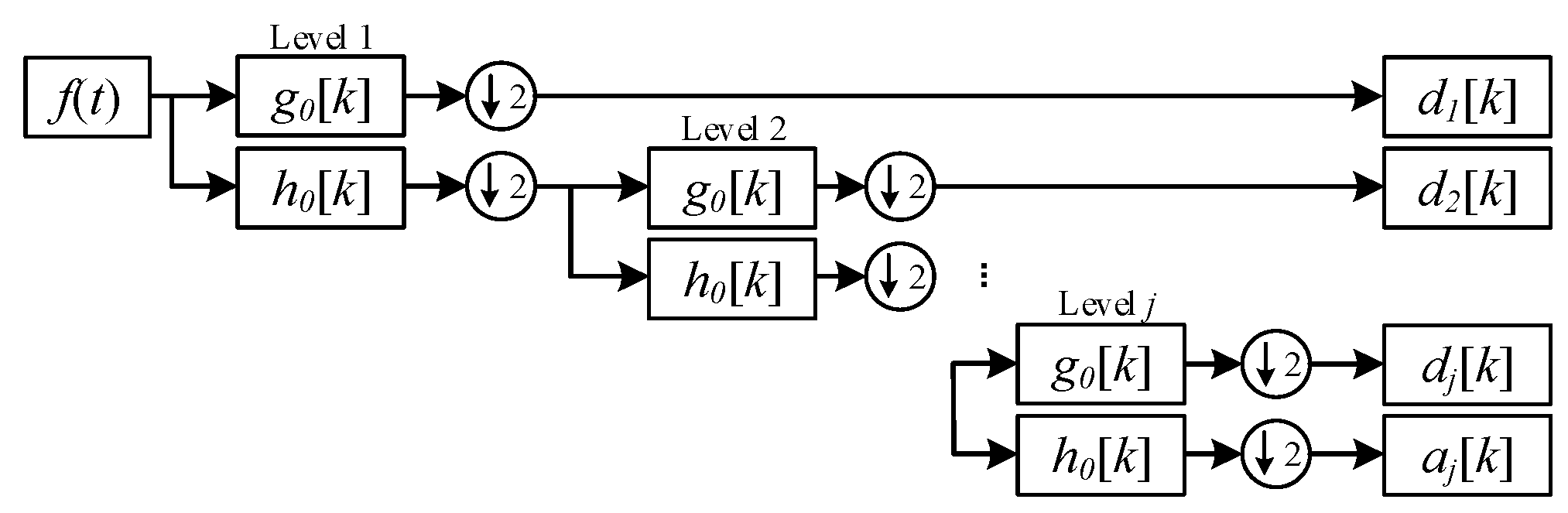
2.2. Multiresolution Analysis (MRA)
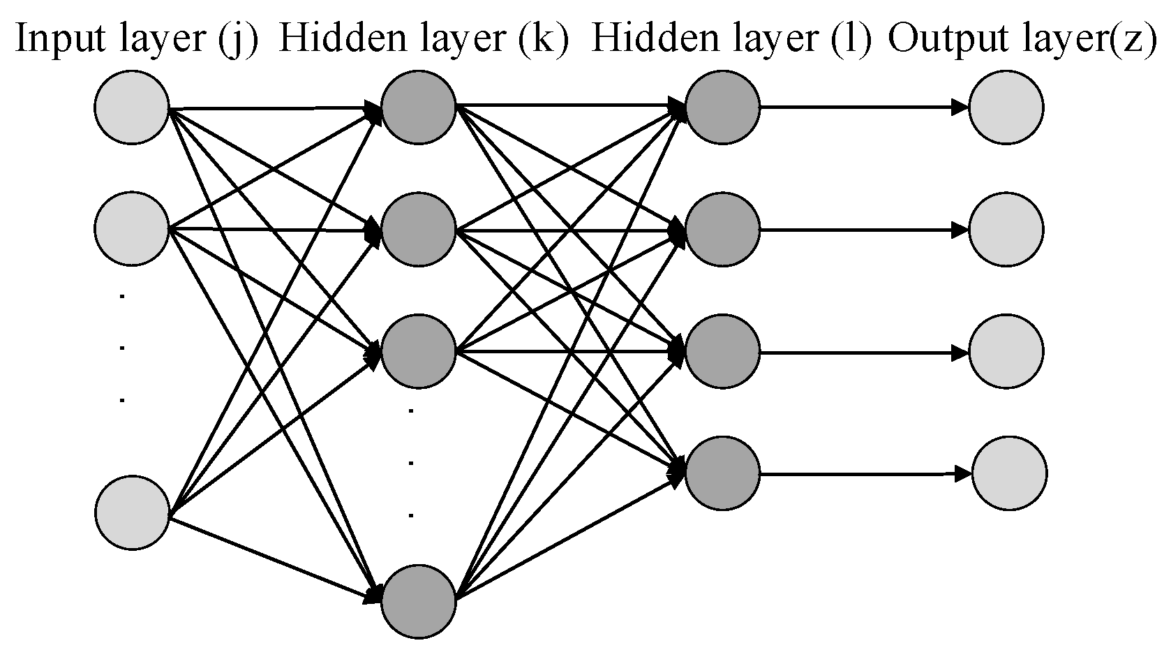
2.3. Artificial Neural Network Training (ANN)
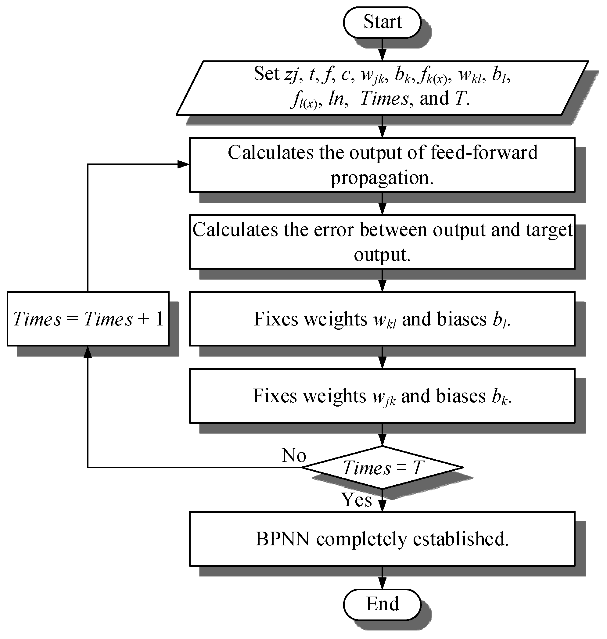
- Step 1.
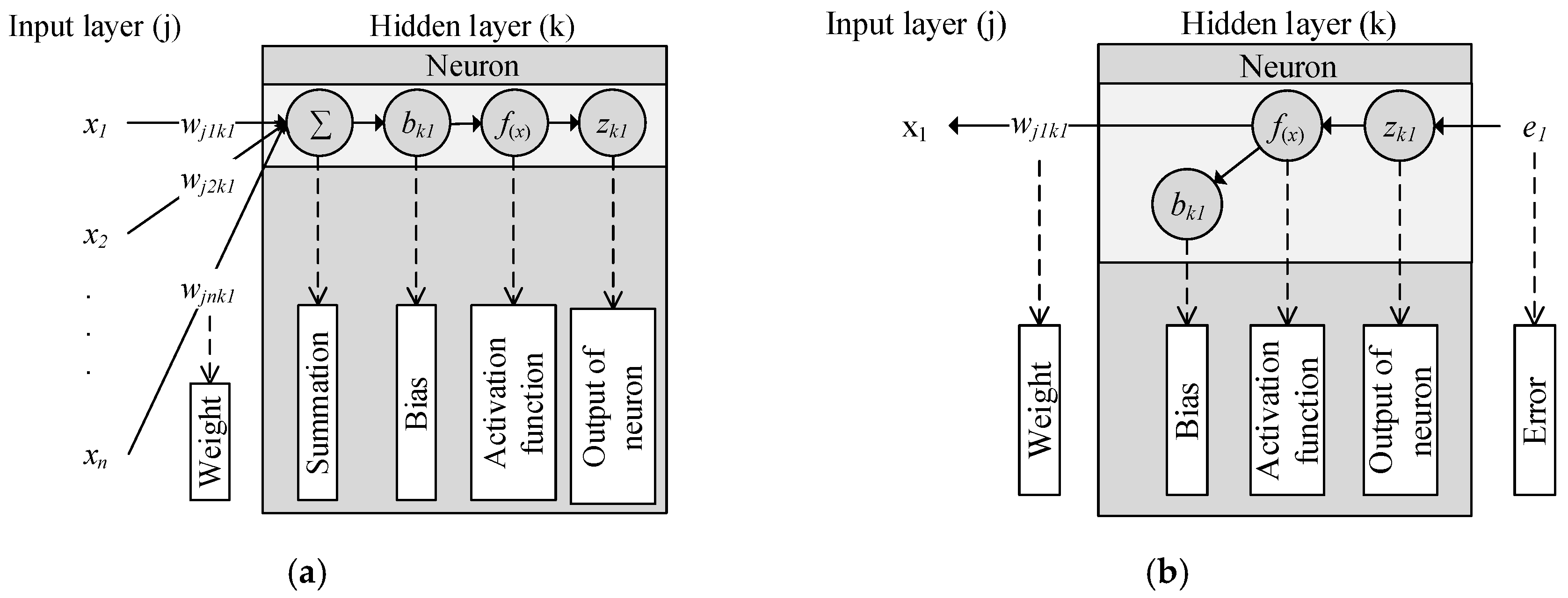
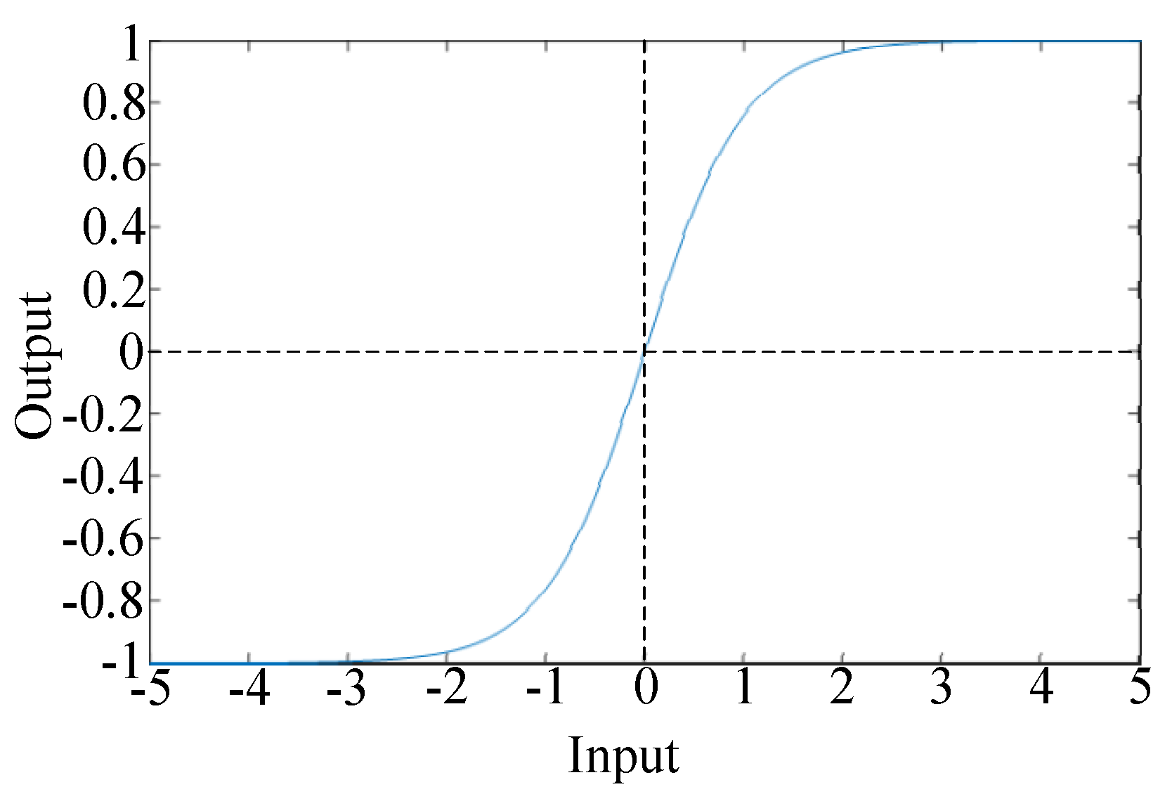
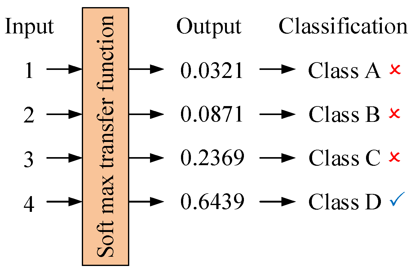
- Set the input data (zj), target output (t), numbers of feature (f), numbers of neurons (c), weights (wjk) between input layer and hidden layer (k), biases (bk) of hidden layer (k), activation function (fk(x)) of hidden layer (k) , weights (wkl) between input layer and hidden layer (l), biases (bl) of hidden layer (l), activation function (fl(x)) of hidden layer (l), learning rate (ln), times of training (Times), times of iteration (T). This study sets c = f + 2, ln = 0.007, T = 50, all the weights and biases are random numbers between 0 and 1, activation function (fk(x)) is hyperbolic tangent sigmoid transfer function [29], activation function (fl(x)) is soft max function [30].where, hyperbolic tangent sigmoid transfer function, shown as (7), limits the output data to −1 and 1, as shown in Figure 4. Softmax function, shown as (8), calculates the input data and let summation of output data equal 1, shown as Figure 5, and the maximum term is regarded as the classification result.
- Step 2.
- Calculate the output (zl) of feed-forward propagation as (9)–(12).
- Step 3.
- Calculate the error (E) between output (zl) and target output (t) by cross entropy, shown as (13).
- Step 4.
- Use stochastic gradient descent algorithm (SGD) to calculate the error about weights (wkl) and biases (bl) from output layer to hidden layer (l) as (14) and (15), fix weights (wkl) and biases (bl) as (16) and (17).
- Step 5.
- Use stochastic gradient descent algorithm (SGD) to fix weights (wjk) and biases (bk), the process is shown as (14)–(17).
- Step 6.
- If Times is not equal T, calculate Times as (18), and back to Step 2.
- Step 7.
- ANN completely established. The flowchart of ANN is shown in Figure 6.
3. Correlation Analysis Algorithm
3.1. Relief
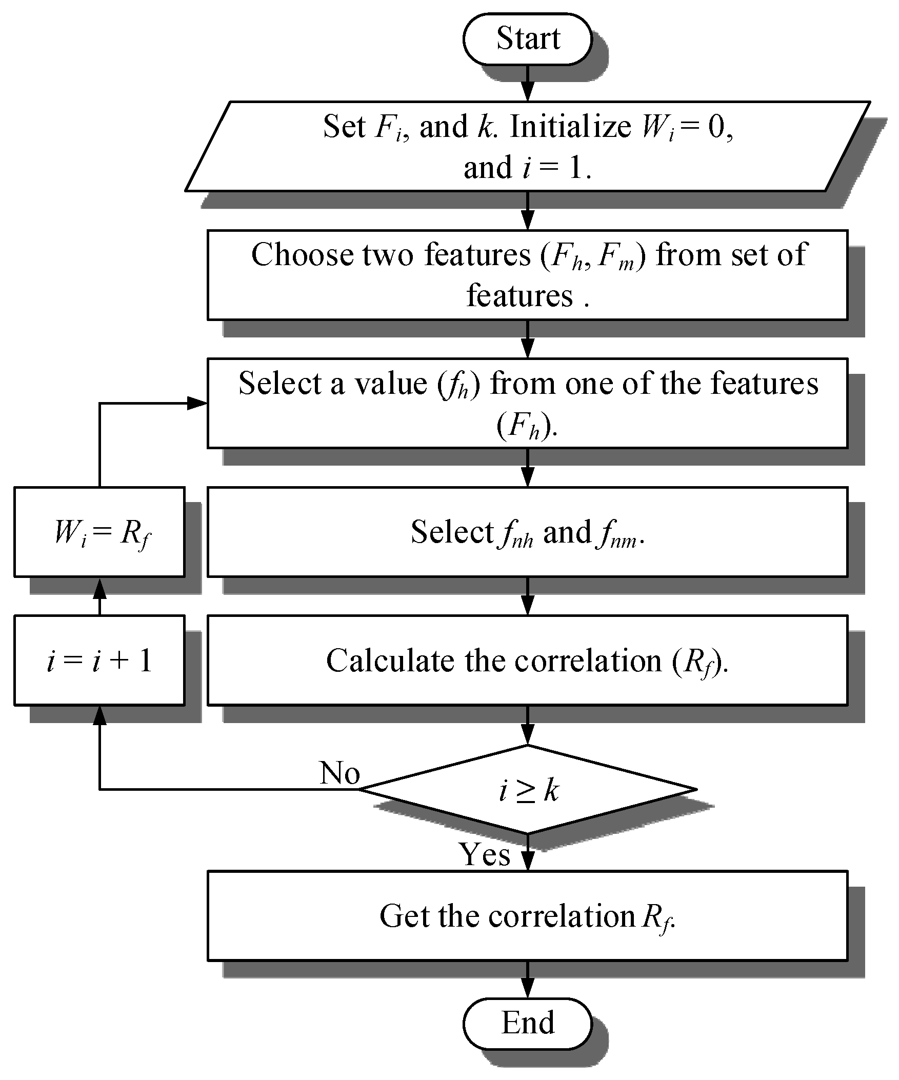
- Step 1.
- Set the set of features (Fi), and maximum times of sampling (k). Initialize the correlation (Wi) to zero, and times of sampling (i) to one. Set of features means all of the features sampling Fi = {F1, F2, ⋯ ⋯, Fp}. Fp is one of the features, value (f1, f2, ⋯ ⋯, ft).
- Step 2.
- Choose two features (Fh, Fm) from set of features.
- Step 3.
- Select one value (fh) from one of the features (Fh).
- Step 4.
- Select one nearest value (fnh) with fh from Fh, and a nearest value (fnm) with Fh from Fm.
- Step 5.
- Calculate the correlation (Rf) with Formula (19),where diff(fh, fnh) is the distance between fh and fnh, diff(fh, fnm) is the distance between fh and fnm.
- Step 6.
- If i ≥ k, select i with Formula (20), and Wi with Formula (21). Go back to Step 3.
- Step 7.
- Get the correlation (Rf) between feature Fh and feature Fm.
3.2. ReliefF
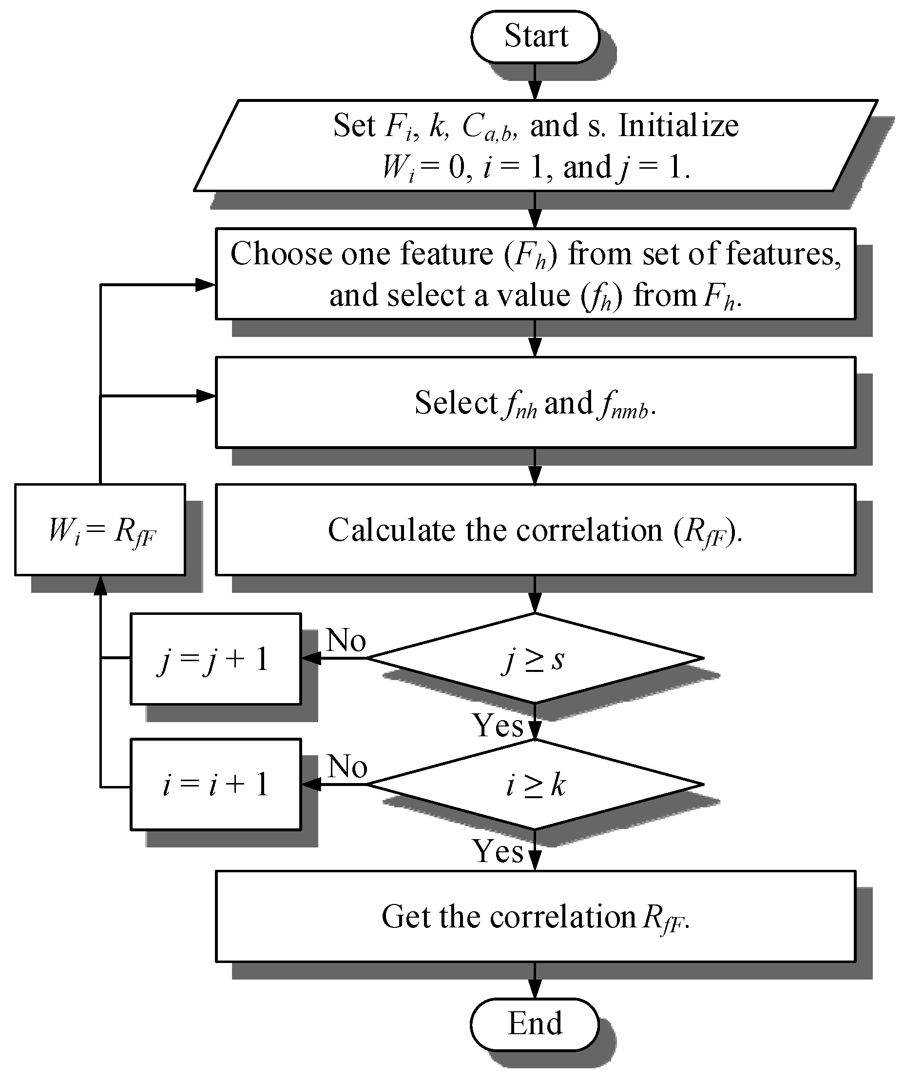
- Step 1.
- Set the set of features (Fi), maximum times of sampling (k), classification of sampling (Ca,b), and the maximum sample number of the nearest value (s). Initialize the correlation (Wi) to zero, times of sampling (i) to one, and sample number of the nearest value (j). The set of features means all of the feature sampling Fi = {F1, F2, ⋯ ⋯, Fp}. Fp is one of the features, value (f1, f2, ⋯ ⋯, ft). Classification of sampling means all of the feature sampling is classification to m class Ca, b = (c1,1, c2,1, ⋯ ⋯, ci,1, c(i+1),2, c(i+2),2, ⋯ ⋯, cj,2, c(j+1),3, ⋯⋯, ct,m), where a is the order about value of feature, b is class b.
- Step 2.
- Choose one feature (Fh) from set of features and select a value (fh) from Fh. fh is belong to n class of all classification (m).
- Step 3.
- Select a nearest value (fnh) with fh from n class of Fh, and the nearest value (fnmb) with fh from each classification of Fh in addition to n class, where fnmb = (fnm1, fnm2, ⋯ ⋯, fnm(n-1), fnm(n+1), ⋯ ⋯, fnmm).
- Step 4.
- Calculate the correlation (RfF) with formula is shown as (22),where diff(fh, fnh) is the distance between fh and fnh, diff(fh, fnmb) is the summation of distance between fh and fnmb.
- Step 5.
- If j ≥ s, select j with Formula (23), and Wi with Formula (24). Go back to Step 3.
- Step 6.
- If i ≥ k, select i with Formula (25), and Wi with Formula (24). Go back to Step 2.
- Step 7.
- Get the correlation (RfF) between feature Fh and classification of sampling (Ca,b).
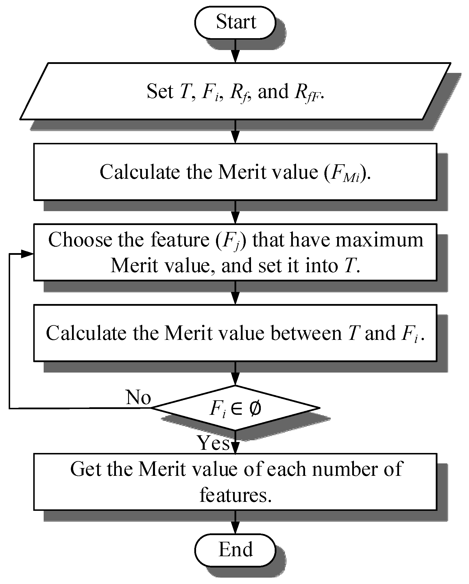
3.3. CFS
- Step 1.
- Set the target of feature T = { }, set of feature Fi = {F1, F2, ⋯⋯, Fn}, correlation between features (Rf), and correlation between feature and classification (RfF) where, Rfij is the correlation between feature Fi and feature Fj, RfFi is the correlation between feature Fi and classification.
- Step 2.
- Calculate the merit value (FMi) based on Rf and RfF with Formula (26) of each feature. FMi = {FM1, FM2, ⋯⋯, FMn}.where, k is number of features (at this step, k = 1), is the average of Rfij, is the average RfFi (at this step, =RfFi).
- Step 3.
- Choose the feature (Fj) that have maximum merit value, set it into T, T = {Fj}, and Fi ⊄ Fj, Fi = {F1, F2, ⋯⋯, F(j-1), F(j+1), ⋯⋯, Fn}.
- Step 4.
- Calculate the merit value between T and Fi with Formula (26).
- Step 5.
- If Fi ≠ ∅, go back to Step 3.
- Step 6.
- Get the merit value of each number of features.
3.4. CFFS
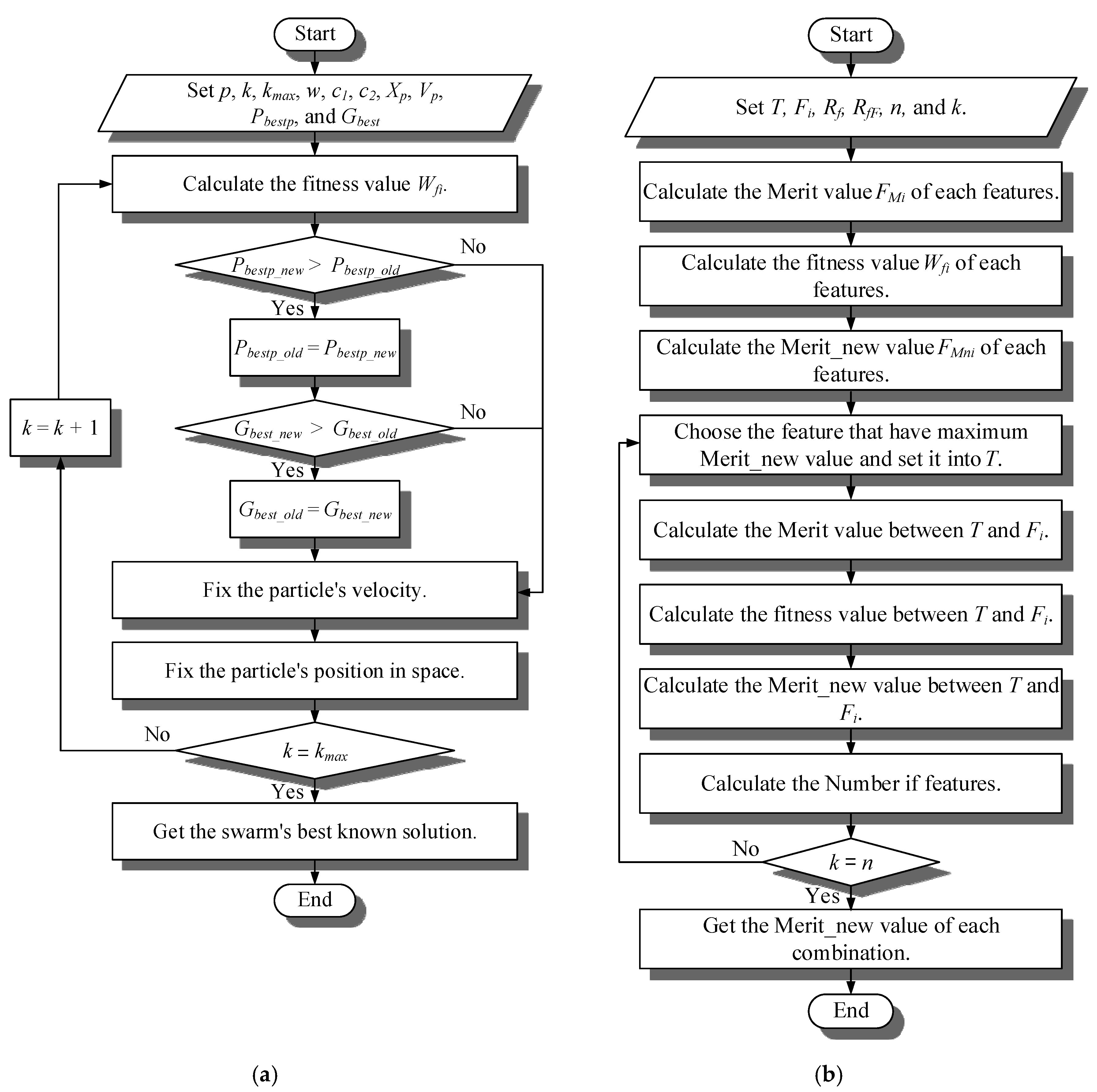
- Step 1.
- Set number of particles (p), number of iterations (k), maximum number of iteration (kmax), inertia weight (w), acceleration constants (c1, c2), particle’s position in space (Xp), particle’s velocity (Vp), particle’s best-known solution (Pbestp), and swarm’s best-known solution (Gbest). Particle’s position in space is means weights of features Xp = (Xp1, Xp2, ⋯⋯, Xpj), particle’s velocity Vp = (Vp1, Vp2, ⋯⋯, Vpj), where j is number of features.
- Step 2.
- Calculate the fitness value (Wfi) of each feature. Fitness value is particle’s accuracy of ANN.
- Step 3.
- Make sure Pbest_new > Pbest_old, replace Pbest_old with Pbest_new as (28), if not, go to Step 5. Pbest_old is particle’s best-known solution before fixed, Pbest_new is particle’s best-known solution after fixed, particle’s best-known solution Pbest = (Pbest1, Pbest2, ⋯⋯, Pbestp).
- Step 4.
- Make sure Gbest_new > Gbest_old, replace Gbest_old with Gbest_new as (29), if not, go to Step 5. Gbest_new is swarm’s best-known solution before fixed, Gbest_new is swarm’s best-known solution after fixed, swarm’s best-known solution is the best solution of particle’s best-known solution.
- Step 5.
- Fix the particle’s velocity as (30) and (31).
- Step 6.
- Fix the particle’s position in space as (32) and (33).
- Step 7.
- Make sure k = kmax, if not, calculates k as (34) and back to Step 2.
- Step 8.
- Get the swarm’s best-known solution for ANN.
- Step 1.
- Set the target of feature T = { }, set of feature Fi = {F1, F2, ⋯⋯, Fn}, correlation between features (Rf), correlation between feature and classification (RfF), number of all features (n), set of feature Fi = {F1, F2, ⋯⋯, Fn}, and number of features k = 1.where, Rfij is the correlation between feature Fi and feature Fj, RfFi is the correlation between feature Fi and classification. Calculate the merit value (FMi) of each features, based on Rf and RfF with Formulas (3)–(8), FMi = {FM1, FM2, ⋯⋯, FMn}, where, k is number of features (at this step, k = 1), is the average of Rfij, is the average RfFi (at this step, =RfFi).
- Step 2.
- Calculate the fitness value (Wfi) of each feature. Fitness value is the accuracy that calculated of artificial neural network. Wfi = (Wf1, Wf2, ⋯⋯, Wfn).
- Step 3.
- Calculate the merit_new value (FMni) with Formula (27) of each feature. FMni = (FMn1, FMn2, ⋯⋯,FMnn).
- Step 4.
- Choose the feature (Fj) that have maximum merit_new value, and set it into T, T = {Fj}. Fi ⊄ Fj, Fi = {F1, F2, ⋯⋯, F(j-l), F(j+l), ⋯⋯, Fn}.
- Step 5.
- Calculate the merit value as Formulas (3)–(8) between T and Fi. FMi = FMi = {FM1, FM2, ⋯⋯, FM(j-l), FM(j+l), ⋯⋯, FMn}.
- Step 6.
- Calculate the fitness value (Wfj) with PSO optimizes the weights of features between T and Fi. Wfi = (Wf1, Wf2, ⋯⋯, Wf(j-l), Wf(j+l), ⋯⋯, Wfn).
- Step 7.
- Calculate the merit_new value as Formula (27) between T and Fi. Choose the feature (Fx) that have maximum merit_new value, and set it into T.
- Step 8.
- Calculate the number of features as (35).
- Step 9.
- Make sure k = n, if not, back to Step 6.
- Step 10.
- Get the merit_new value of each combination of number of features.
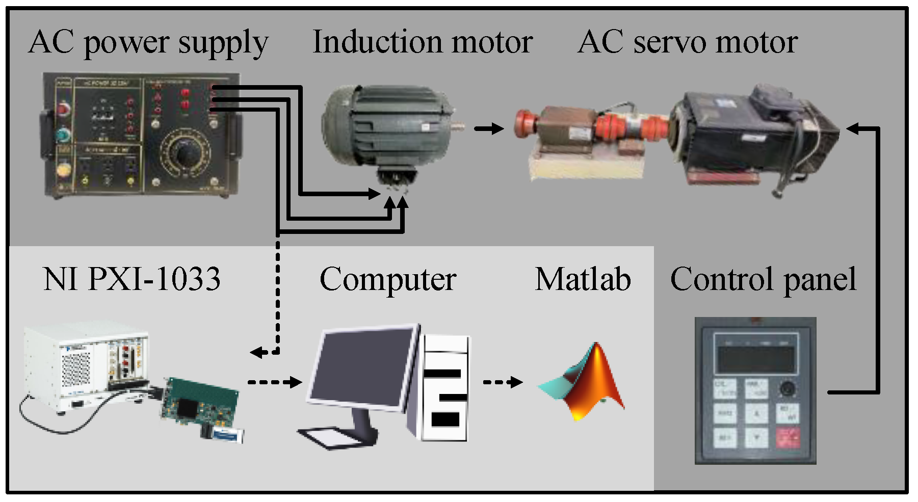
4. Measurement and Analysis of the Current Signal of the Induction Motor
- Step 1.
- Prepare all the samples of the motor. This study prepares four classes of motor: normal, damage of shaft output of bearing, layer short, and broken rotor bar.
- Step 2.
- Connect the three phases R, S, and T of motor with AC power supply. R, S, and T are same AC power but have different angle.
- Step 3.
- Setup the NI PXI-1033 and computer and choose one of the three phases to measure current signal.
- Step 4.
- Use AC power supply to input the power to the motor.
- Step 5.
- Use control panel to select torque of AC servo motor to simulate the load of the motor. This study selected the half load for the motor.
- Step 6.
- Use Labview to record data from NI PXI-1033.
- Step 7.
- Use Matlab to analyze the current signal of each motor.
5. Classification of Induction Motor Failure
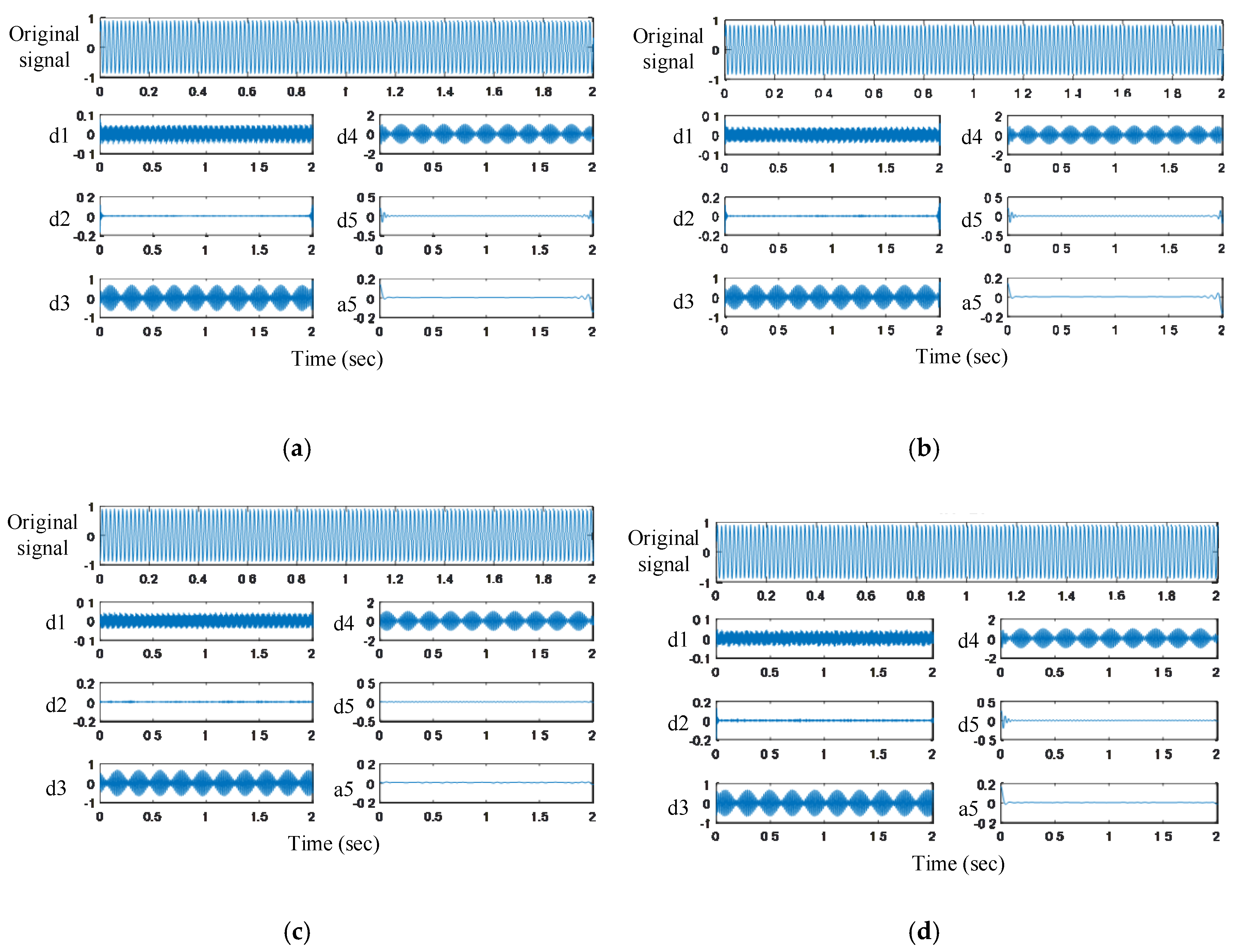
5.1. Motorcurrent Signal Analysis of Induction Motor Failure
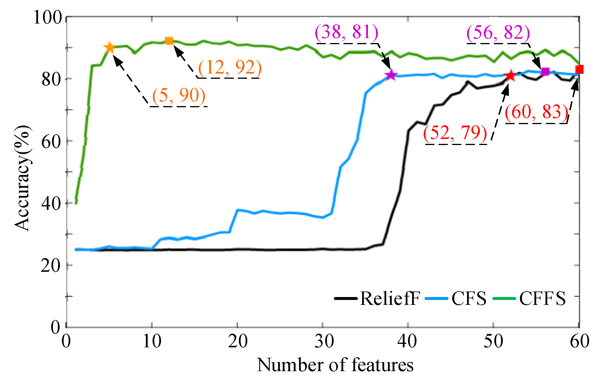
5.2. Accuracy of Classifier
- (1)
- ReliefF:
- (2)
- CFS:
- (3)
- CFFS:
6. Conclusions
Author Contributions
Funding
Conflicts of Interest
References
- Zhang, P.Y.; Shu, S.; Zhou, M. An online fault detection model and strategies based on SVM-grid in clouds. IEEE/CAA J. Autom. Sin. 2018, 5, 445–456. [Google Scholar] [CrossRef]
- Wang, H.; Lu, S.; Qian, G.; Ding, J.; Liu, Y.; Wang, Q. A two-step strategy for online fault detection of high-resistance connection in BLDC motor. IEEE Trans. Power Electron. 2020, 35, 3043–3053. [Google Scholar] [CrossRef]
- Mao, W.; Chen, J.; Liang, X.; Zhang, X. A new online detection approach for rolling bearing incipient fault via self-adaptive deep feature matching. IEEE Trans. Instrum. Meas. 2020, 69, 443–456. [Google Scholar] [CrossRef]
- Bazurto, A.J.; Quispe, E.C.; Mendoza, R.C. Causes and failures classification of industrial electric motor. In Proceedings of the 2016 IEEE ANDESCON, Arequipa, Peru, 19–21 October 2016. [Google Scholar]
- Kral, C.; Habetler, T.G.; Harley, R.G.; Pirker, F.; Pascoli, G.; Oberguggenb, H.; Fenz, C.J.M. A comparison of rotor fault detection techniques with respect to the assessment of fault severity. In Proceedings of the 4th IEEE International Symposium on Diagnostics for Electric Machines, Power Electronics and Drives, Atlanta, GA, USA, 24–26 August 2003; pp. 265–269. [Google Scholar]
- Liu, W.; Liao, Q.; Qiao, F.; Xia, W.; Wang, C.; Lombardi, F. Approximate designs for fast Fourier transform (FFT) with application to speech recognition. IEEE Trans. Circuits Syst. I Regul. Pap. 2019, 66, 4727–4739. [Google Scholar] [CrossRef]
- Pei, S.C.; Ding, J.J. Relations between Gabor transforms and Fractional Fourier Transforms and their applications for signal processing. IEEE Trans. Signal Process. 2007, 55, 4839–4850. [Google Scholar] [CrossRef]
- Cho, S.H.; Jangand, G.; Kwon, S.H. Time-frequency analysis of power-quality disturbances via the Gabor–Wigner transform. IEEE Trans. Power Deliv. 2010, 25, 494–499. [Google Scholar]
- Laurence, C.; Pierre-Francois, M.; Lise, D.; Kim, P.G.; Francis, G.; Sá, R.C. A method for the analysis of respiratory sinus arrhythmia using continuous wavelet transforms. IEEE Trans. Biomed. Eng. 2008, 55, 1640–1642. [Google Scholar]
- Ghunem, R.A.; Jayaram, S.H.; Cherney, E.A. Investigation into the eroding dry-band arcing of filled silicone rubber under DC using wavelet-based multiresolution analysis. IEEE Trans. Dielectr. Electr. Insul. 2014, 21, 713–720. [Google Scholar] [CrossRef]
- Kang, M.; Kim, J.; Wills, L.M.; Kim, J.M. Time-varying and multiresolution envelope analysis and discriminative feature analysis for bearing fault diagnosis. IEEE Trans. Ind. Electron. 2015, 62, 7749–7761. [Google Scholar] [CrossRef]
- Ananthan, S.N.; Padmanabhan, R.; Meyur, R.; Mallikarjuna, B.; Reddy, M.J.B.; Mohanta, D.K. Real-time fault analysis of transmission lines using wavelet multi-resolution analysis based frequency-domain approach. IET Sci. Meas. Technol. 2016, 10, 693–703. [Google Scholar] [CrossRef]
- Bíscaro, A.A.P.; Pereira, R.A.F.; Kezunovic, M.; Mantovani, J.R.S. Integrated fault location and power-quality analysis in electric power distribution systems. IEEE Trans. Power Deliv. 2016, 31, 428–436. [Google Scholar]
- Al-Otaibi, R.; Jin, N.; Wilcox, T.; Flach, P. Feature construction and calibration for clustering daily load curves from smart-meter data. IEEE Trans. Ind. Inform. 2016, 12, 645–654. [Google Scholar] [CrossRef]
- Imani, M.; Ghassemian, H. Band clustering-based feature extraction for classification of hyperspectral images using limited training samples. IEEE Geosci. Remote Sens. Lett. 2014, 11, 1325–1329. [Google Scholar] [CrossRef]
- Neshatian, K.; Zhang, M.; Andreae, P. A filter approach to multiple feature construction for symbolic learning classifiers using genetic programming. IEEE Trans. Evolut. Comput. 2012, 16, 645–661. [Google Scholar] [CrossRef]
- Panigrahy, P.S.; Santra, D.; Chattopadhyay, P. Feature engineering in fault diagnosis of induction motor. In Proceedings of the 2017 3rd International Conference on Condition Assessment Techniques in Electrical Systems (CATCON), Rupnagar, India, 16–18 November 2017. [Google Scholar]
- Godse, R.; Bhat, S. Mathematical morphology-based feature-extraction technique for detection and classification of faults on power transmission line. IEEE Access 2020, 8, 38459–38471. [Google Scholar] [CrossRef]
- Rauber, T.W.; de Assis Boldt, F.; Varejão, F.M. Heterogeneous feature models and feature selection applied to bearing fault diagnosis. IEEE Trans. Ind. Electron. 2014, 62, 637–646. [Google Scholar] [CrossRef]
- Fu, R.; Wang, P.; Gao, Y.; Hua, X. A new feature selection method based on Relief and SVM-RFE. In Proceedings of the 2014 12th International Conference on Signal Processing (ICSP), Hangzhou, China, 19–23 October 2014. [Google Scholar]
- Fu, R.; Wang, P.; Gao, Y.; Hua, X. A combination of Relief feature selection and fuzzy k-nearest neighbor for plant species identification. In Proceedings of the 2016 International Conference on Advanced Computer Science and Information Systems (ICACSIS), Malang, Indonesia, 15–16 October 2016. [Google Scholar]
- Huang, Z.; Yang, C.; Zhou, X.; Huang, T. A hybrid feature selection method based on binary state transition algorithm and ReliefF. IEEE J. Biomed. Health Inform. 2019, 23, 1888–1898. [Google Scholar] [CrossRef]
- Hu, B.; Li, X.; Sun, S.; Ratcliffe, M. Attention recognition in EEG-based affective learning research using CFS+knn algorithm. IEEE/ACM Trans. Comput. Biol. Bioinform. 2018, 15, 38–45. [Google Scholar] [CrossRef]
- Singh, A.; Thakur, N.; Sharma, A. A review of supervised machine learning algorithms. In Proceedings of the 2016 3rd International Conference on Computing for Sustainable Global Development (INDIACom), New Delhi, India, 16–18 March 2016. [Google Scholar]
- Bao, F.; Maier, T. Stochastic gradient descent algorithm for stochastic optimization in solving analytic continuation problems. Am. Inst. Math. Sci. Found. Data Sci. 2020, 2, 1–17. [Google Scholar] [CrossRef]
- Wu, W.; Feng, G.R.; Li, Z.X. Deterministic convergence of an online gradient method for BP neural networks. IEEE Trans. Neural Netw. 2005, 16, 533–540. [Google Scholar] [CrossRef]
- Park, D.J.; Jun, B.E.; Kim, J.H. Novel training algorithm for multilayer feedforward neural network. Electron. Lett. 1992, 28, 543–544. [Google Scholar] [CrossRef]
- Rumelhart, D.E.; Hinton, G.E.; Williams, R.J. Learning internal representations by error backpropagation. In Parallel Distributed Processing; Rumelhart, D.E., McClelland, J.L., Eds.; Stanford University: Stanford, CA, USA, 1986; Volume 1, pp. 319–362. [Google Scholar]
- Popoola, S.I.; Jefia, A.; Atayero, A.A.; Kingsley, O.; Faruk, N.; Oseni, O.F.; Abolade, R.O. Determination of neural network parameters for path loss prediction in very high frequency wireless channel. IEEE Access 2019, 7, 150462–150483. [Google Scholar] [CrossRef]
- Sangari, A.; Sethares, W. Convergence analysis of two loss functions in soft-max regression. IEEE Trans. Signal Process. 2016, 64, 1280–1288. [Google Scholar] [CrossRef]
- Lee, C.Y.; Tuegeh, M. An optimal solution for smooth and non-smooth cost functions-based economic dispatch proble. Energies 2020, 13, 3721. [Google Scholar] [CrossRef]
- Juan Luis, F.M.; Esperanza, G.G. Stochastic stability analysis of the linear continuous and discrete PSO models. IEEE Trans. Evolut. Comput. 2011, 15, 405–423. [Google Scholar]


| Induction Motor | |||
|---|---|---|---|
| Rated voltage | 220 V | Power frequency | 60 Hz |
| Output | 2 Hp | Rated speed | 1764 rpm |
| Number of poles | 4 poles | Power factor | 0.8 |
| a5 | d5 | d4 | d3 | d2 | d1 | |
|---|---|---|---|---|---|---|
| Tmax | F1 | F2 | F3 | F4 | F5 | F6 |
| Tmin | F7 | F8 | F9 | F10 | F11 | F12 |
| Tmean | F13 | F14 | F15 | F16 | F17 | F18 |
| Tmse | F19 | F20 | F21 | F22 | F23 | F24 |
| Tstd | F25 | F26 | F27 | F28 | F29 | F30 |
| Fmax | F31 | F32 | F33 | F34 | F35 | F36 |
| Fmin | F37 | F38 | F39 | F40 | F41 | F42 |
| Fmean | F43 | F44 | F45 | F46 | F47 | F48 |
| Fmse | F49 | F50 | F51 | F52 | F53 | F54 |
| Fstd | F55 | F56 | F57 | F58 | F59 | F60 |
| Feature Numbers | Accuracy | The Elements of the Feature Vector |
|---|---|---|
| 37 | 26.81% | F1, F2, F4, …, F8, F10, F11, F12, F14, …, F20, F25, F26, F31, F32, F37, …, F50, F55, F56 |
| 38 | 35.85% | F1, F2, F4, …, F8, F10, F11, F12, F13, F14, …, F20, F25, F26, F31, F32, F37, …, F50, F55, F56 |
| 39 | 43.97% | F1, F2, F4, …, F8, F10, F11, F12, F13, F14, …, F20, F25, F26, F29, F31, F32, F37, …, F50, F55, F56 |
| 40 | 63.35% | F1, F2, F4, …, F8, F9, F10, F11, F12, F13, F14, …, F20, F25, F26, F29, F31, F32, F37, …, F50, F55, F56 |
| 42 | 65.44% | F1, F2, F4, …, F20, F23, F25, F26, F29, F31, F32, F37, …, F50, F53, F55, F56 |
| 43 | 71.45% | F1, F2, F3, F4, …, F20, F23, F25, F26, F29, F31, F32, F37, …, F50, F53, F55, F56 |
| Feature Numbers | Accuracy | The Elements of the Feature Vector |
|---|---|---|
| 19 | 30.58% | F1, F2, F8, F10, F11, F14, F15, F17, …, F20, F31, F38, …, F41, F47, F49, F50 |
| 20 | 37.85% | F1, F2, F8, F10, F11, F14, F15, F17, …, F20, F31, F32, F38, …, F41, F47, F49, F50 |
| 31 | 36.78% | F1, F2, F8, F10, F11, F14, F15, F17, …, F20, F25, F26, F31, F32, F37, …, F50, F55, F56 |
| 32 | 51.56% | F1, F2, F8, F10, F11, F14, F15, F17, …, F20, F25, F26, F29, F31, F32, F37, …, F50, F55, F56 |
| 33 | 54.4% | F1, F2, F8, F10, F11, F14, F15, F17, …, F20, F25, F26, F29, F31, F32, F37, …, F50, F53, F55, F56 |
| 34 | 60.58% | F1, F2, F8, F10, F11, F14, F15, F17, …, F20, F25, F26, F29, F31, F32, F37, …, F50, F53, F55, F56, F59 |
| 35 | 75.46% | F1, F2, F8, F10, F11, F14, F15, F17, …, F20, F25, F26, F29, F31, F32, F37, …, F50, F52, F53, F55, F56, F59 |
| Feature Numbers | Accuracy | The Elements of the Feature Vector |
|---|---|---|
| 1 | 39.5% | F6 |
| 2 | 55.5% | F6, F34 |
| 3 | 84.25% | F6, F34, F57 |
| 4 | 84.5% | F6, F34, F52, F57 |
| 5 | 90% | F6, F34, F35, F52, F57 |
© 2020 by the authors. Licensee MDPI, Basel, Switzerland. This article is an open access article distributed under the terms and conditions of the Creative Commons Attribution (CC BY) license (http://creativecommons.org/licenses/by/4.0/).
Share and Cite
Lee, C.-Y.; Wen, M.-S. Establish Induction Motor Fault Diagnosis System Based on Feature Selection Approaches with MRA. Processes 2020, 8, 1055. https://doi.org/10.3390/pr8091055
Lee C-Y, Wen M-S. Establish Induction Motor Fault Diagnosis System Based on Feature Selection Approaches with MRA. Processes. 2020; 8(9):1055. https://doi.org/10.3390/pr8091055
Chicago/Turabian StyleLee, Chun-Yao, and Meng-Syun Wen. 2020. "Establish Induction Motor Fault Diagnosis System Based on Feature Selection Approaches with MRA" Processes 8, no. 9: 1055. https://doi.org/10.3390/pr8091055
APA StyleLee, C.-Y., & Wen, M.-S. (2020). Establish Induction Motor Fault Diagnosis System Based on Feature Selection Approaches with MRA. Processes, 8(9), 1055. https://doi.org/10.3390/pr8091055