Optimal Non-Convex Combined Heat and Power Economic Dispatch via Improved Artificial Bee Colony Algorithm


Abstract
1. Introduction
1.1. Motivation and Problem Statement
1.2. Review of Related Works
1.3. Contributions
- 1.
- Proposing an improved version of artificial bee colony algorithm for dealing with non-convex optimization problems.
- 2.
- Studying the effectiveness and performance of the proposed algorithm using normal and large-scale test systems and benchmark functions.
- 3.
- Implementation of the proposed algorithm on CHPED problem with different sizes and characteristics.
- 4.
- Compared with available methods in the literature, achieving feasible and better results for large-scale CHPED test systems.
1.4. Paper Organization
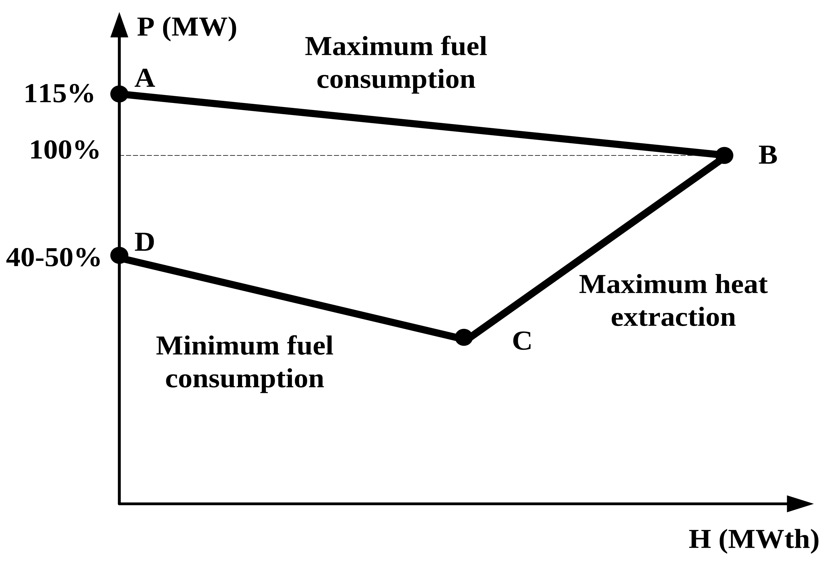
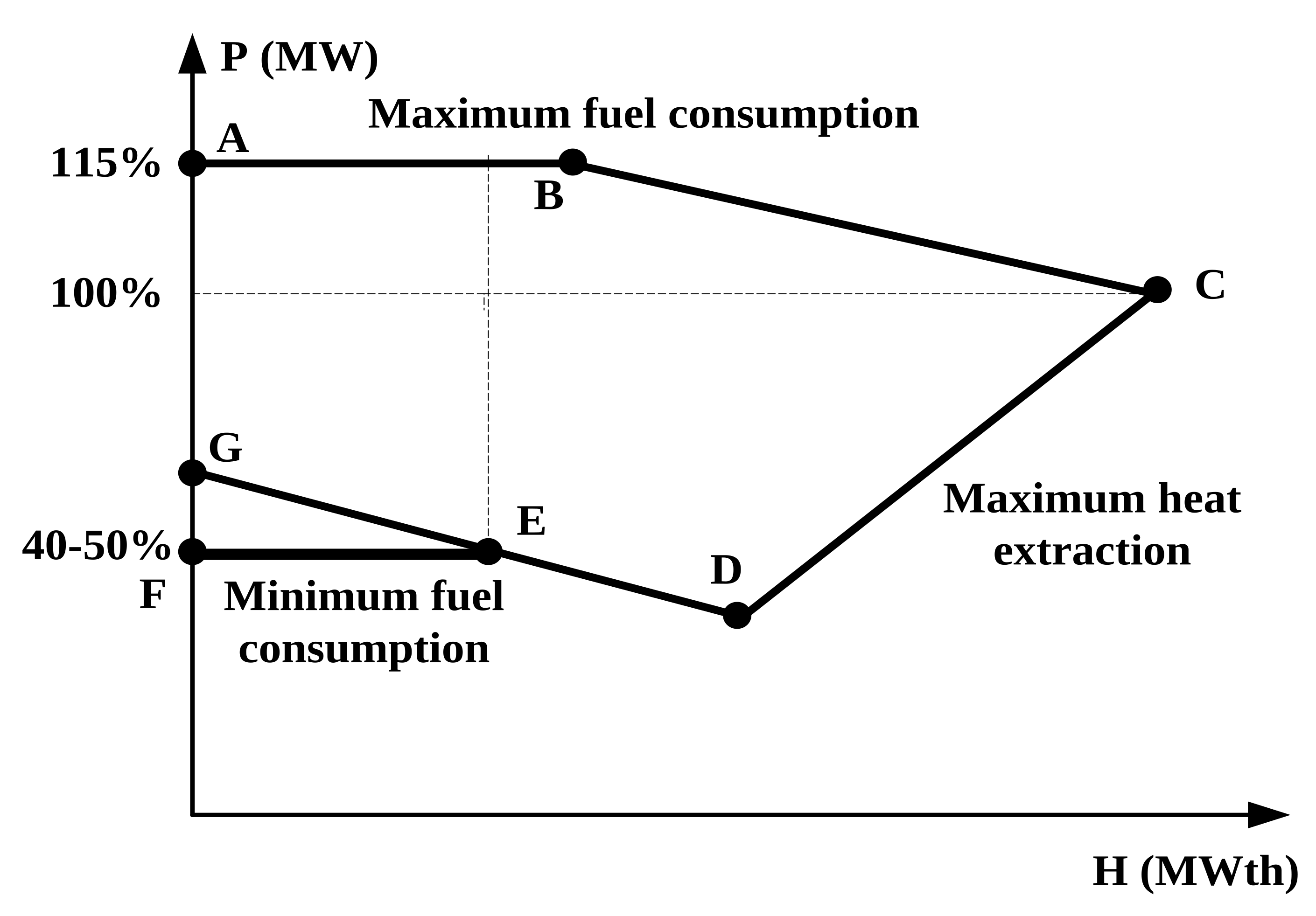
2. Chp Economic Dispatch Problem Formulation
3. Improved Artificial Bee Colony Algorithm
3.1. Original Abc Algorithm
- 1.
- Employed bees discover food sources and determine the quality of nectar and share its location with others bees.
- 2.
- Onlooker bees decide based on the quality of the food sources found by employed bees and follow the location of food sources of employed bees.
- 3.
- If the food source of an employed bee is abandoned, it becomes scout bee and discover new food source randomly.
3.2. Improved Abc (Iabc) Algorithm
- 1.
- As it is observed from Equation (21), as the difference between and decreases, the disturbance of position decreases. Therefore, the length of step is adaptively reduced by approaching to an optimal solution, and hence the algorithm converges to the optimal solution.
- 2.
- It is observed from Equation (18) that the algorithm automatically jumps form local optimal or even non-optimal points, since scout bees are generated when no progress made in the search for a specified food source (or solution).
- 3.
- Onlooker bees capability included in this algorithm enables comparison of the behavior of all food sources (or solutions) simultaneously. In other words, it is observed from Equation (17) that if a specified solution (or food source) i has a small , then it is a good solution, and hence it is not updated by onlooker bees. Otherwise, it is replaced with new position by onlooker bees.
4. Investigation of Iabc Algorithm on the Benchmark Functions
4.1. Study-I: Investigations on Six Benchmark Functions
4.2. Study-Ii: Investigations on Large-Scale Benchmark Functions
5. Implementation of Iabc on the Chped Problem
- 1.
- Step-1: The first stage in IABC algorithm is initialization of the employed bees. Every food source location is a candidate solution of CHPED problem. The position of each food source () is a vector of all real power and heat outputs of the units as presented in the following.
- 2.
- Step-2: By setting (where is the iteration number of the algorithm), discover new food source locations by employed bees using Equation (21).
- 3.
- Step-3: In this step the objective function value for the population of bees are calculated at the current iteration. Since the CHPED is a constrained optimization problem, it is converted to an unconstrained problem using penalty coefficient (). is assumed to be 10000 for all test systems studied in the following section. Hence, the objective function will be as follows.
- 4.
- Step-4: Fitness of i-th food source is calculated from Equation (16). If the new food source fitness is better than the old, then the old food source is replaced with the new location (obtained in Step-2, and ( is a counter that determines limit value for converting i-th employed bee to scout bee), otherwise old location is preserved and .
- 5.
- Step-5: At this step onlooker bees select food source of employed bees by using the roulette wheel criterion given in (17). Based on the value of for each food source, the onlooker bees modify the selected locations of employed bees by using (21), as follows: If , then the fitness of new food source is calculated from (16). If it is better than old fitness value, the old food source is replaced with new location and , otherwise the old food location is kept and .
- 6.
- Step-6: After the completion of the food source update process for employed and onlooker bees, if , then that food source is abandoned, and the employed bee is converted to a scout bee. The scout bee selects its new food source randomly in the space via (18).
- 7.
- Step-7: Check the stopping criterion. If the algorithm converged, then go to Step-8, else and go to Step-2 and repeat the above procedure. In this paper, the stopping criterion is reaching to the maximum number of iterations in each run. In other words, if , then the algorithm stopped.
- 8.
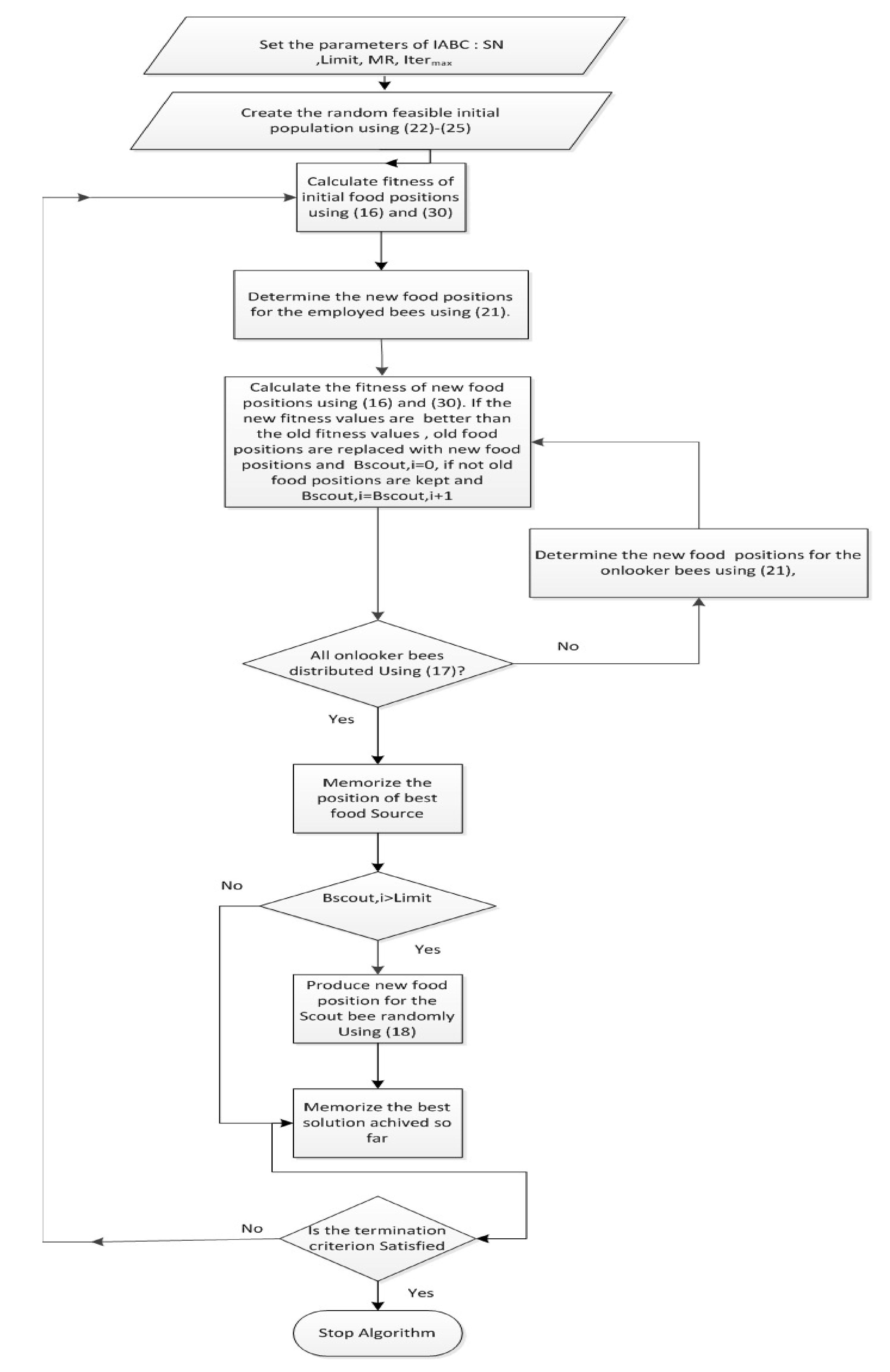
- Step-8: Stop. To clarify the optimization process for energy engineers, the implemented method is presented in Figure 3.
6. Case Studies
6.1. Test System I (7-Unit System)
6.1.1. Case I
6.1.2. Case II
6.1.3. Case III
6.2. Test System Ii (24-Unit System)
6.3. Test System Iii (48-Unit System)
7. Conclusions
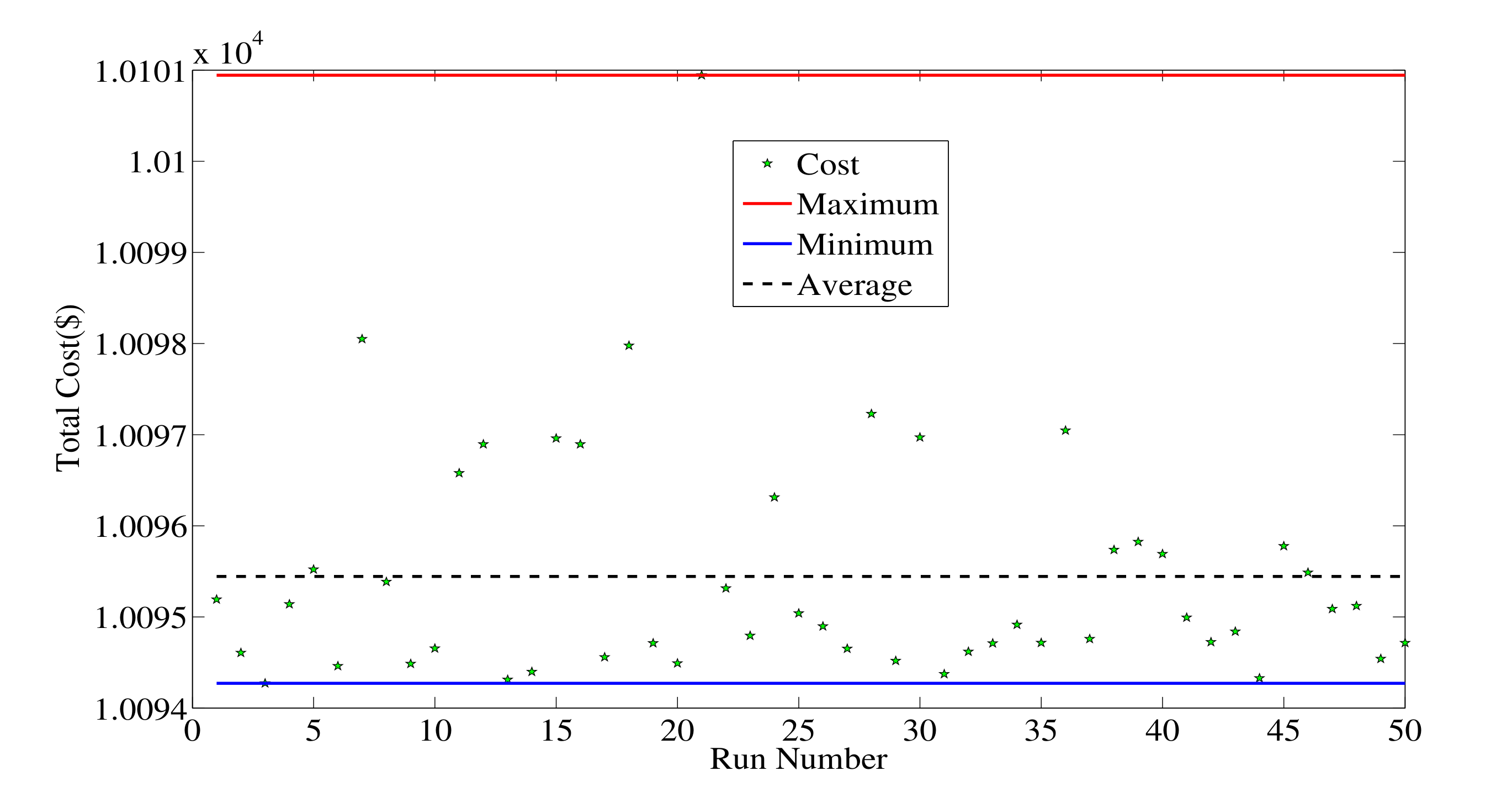
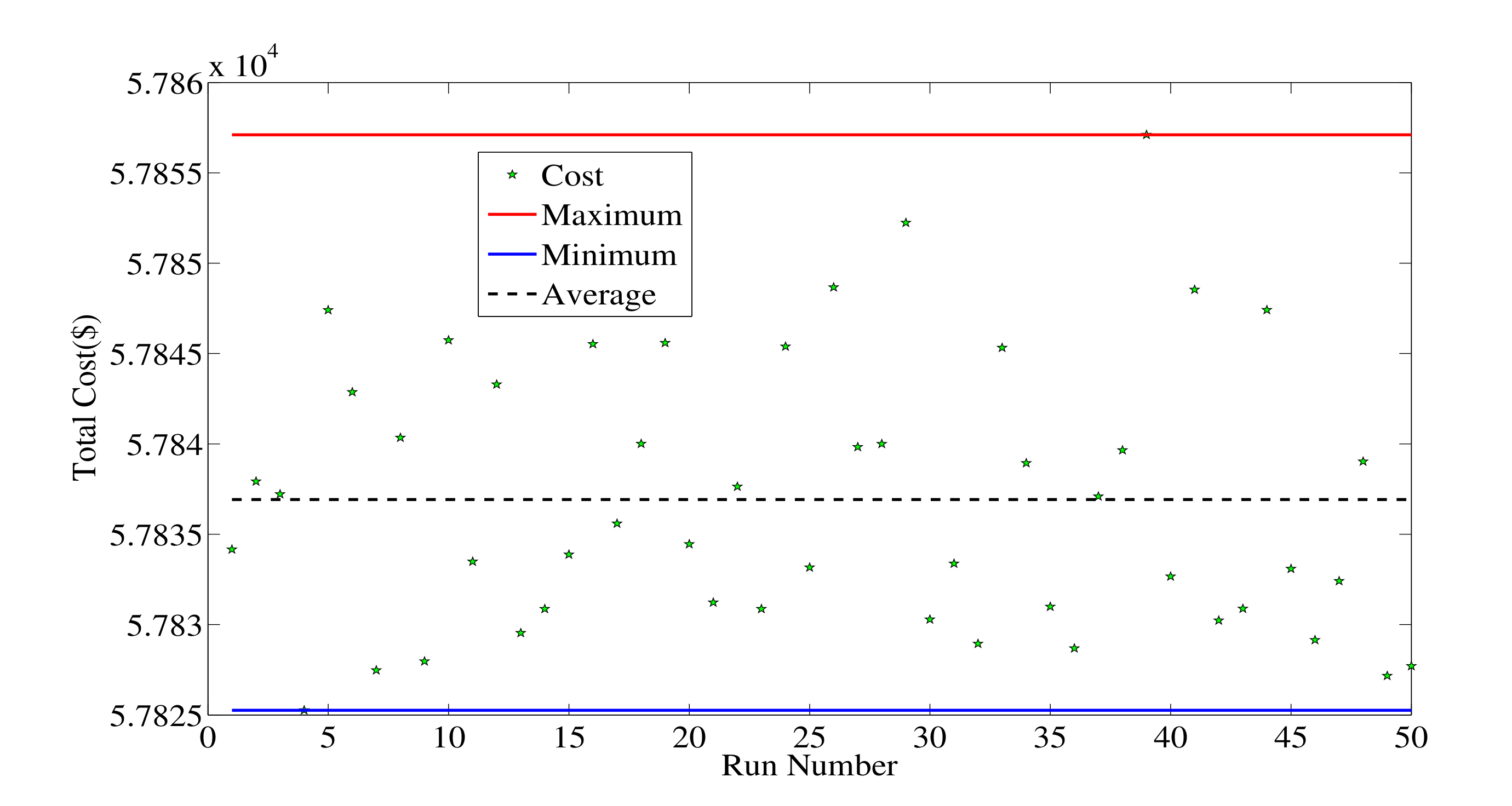
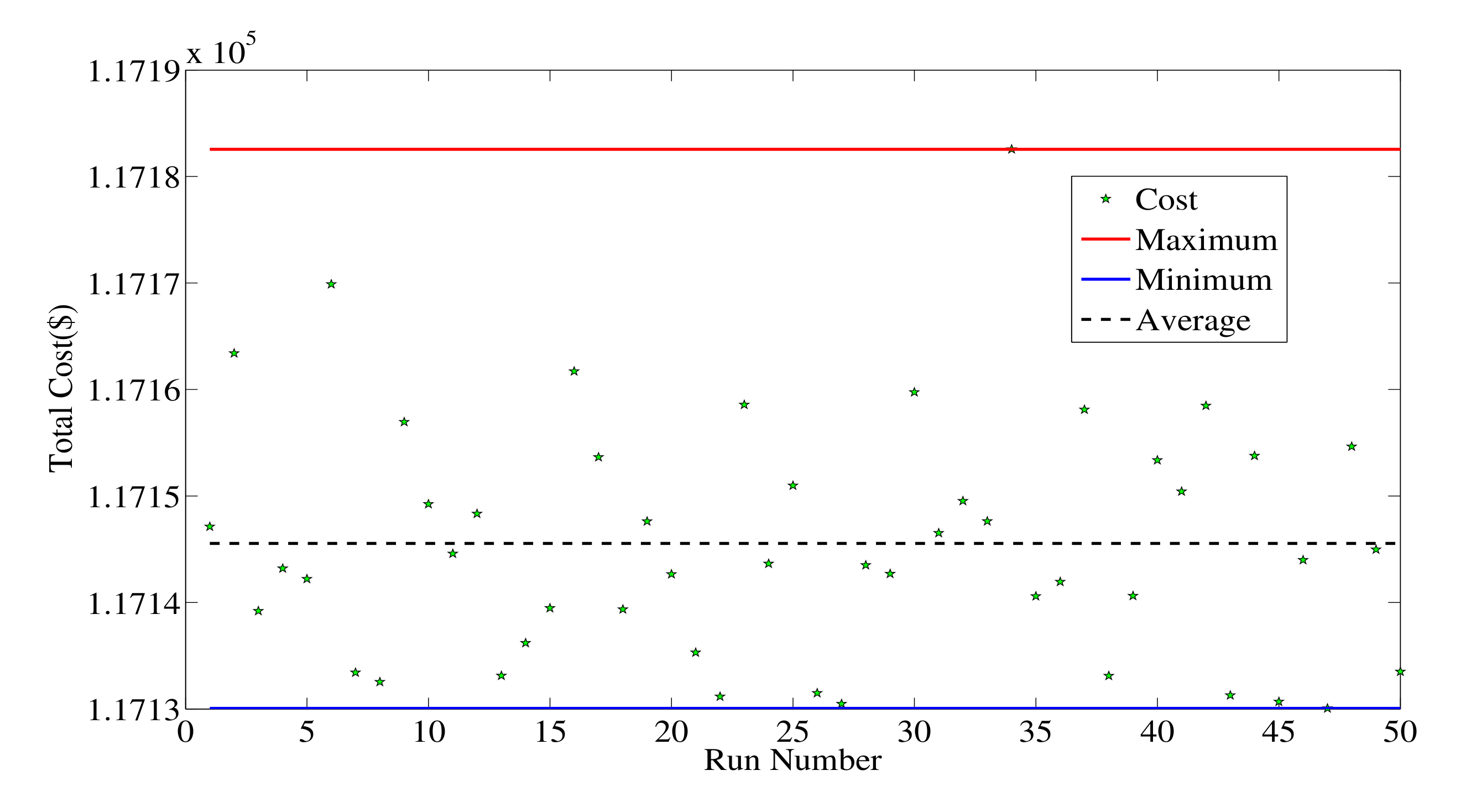
- The obtained results by the proposed IABC algorithm has small diversity and in most cases the algorithm converges to optimal or near optimal solutions. In other words, the variance of the obtained solutions is small.
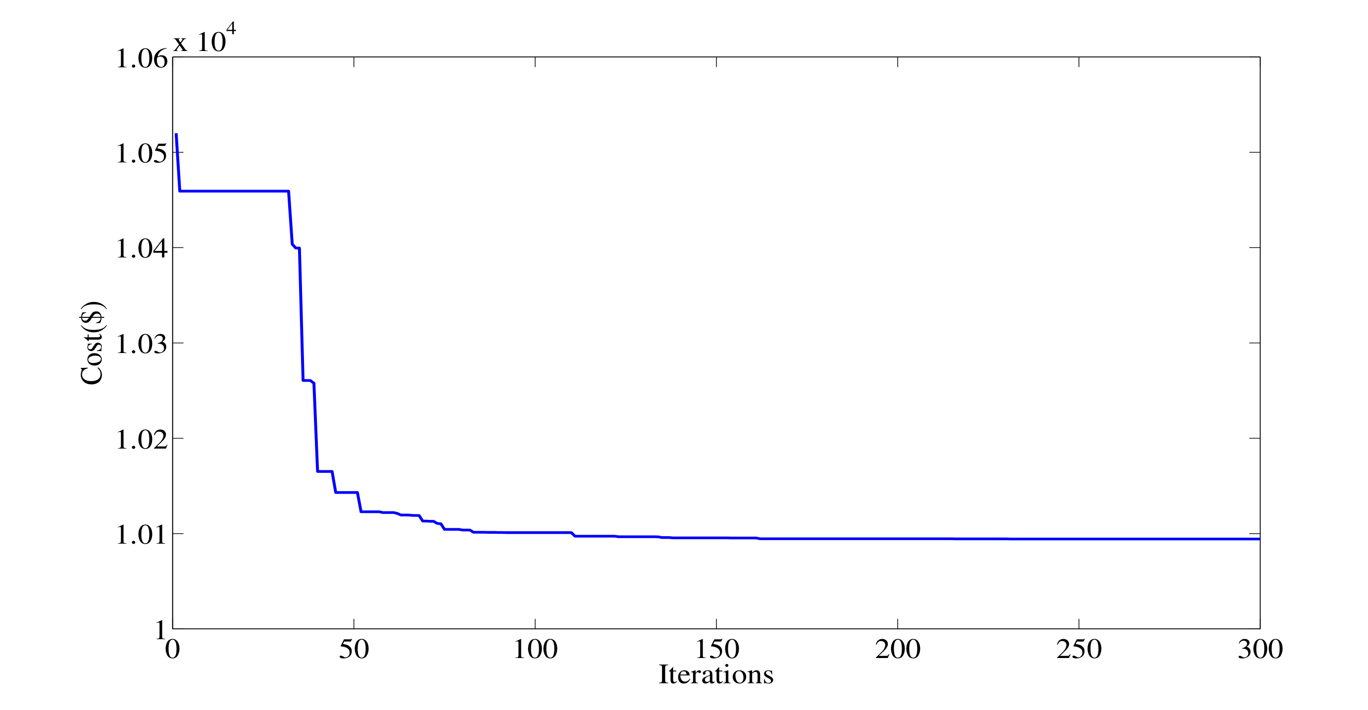
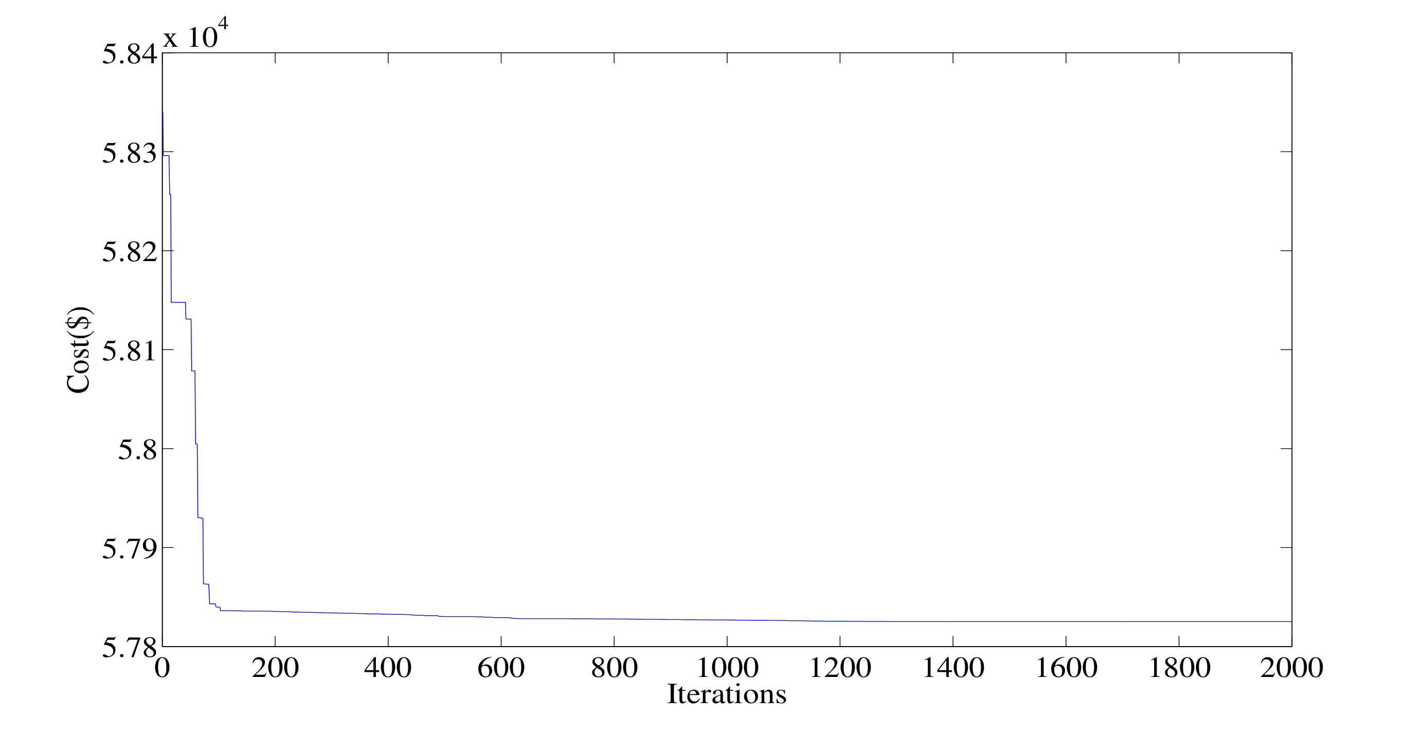
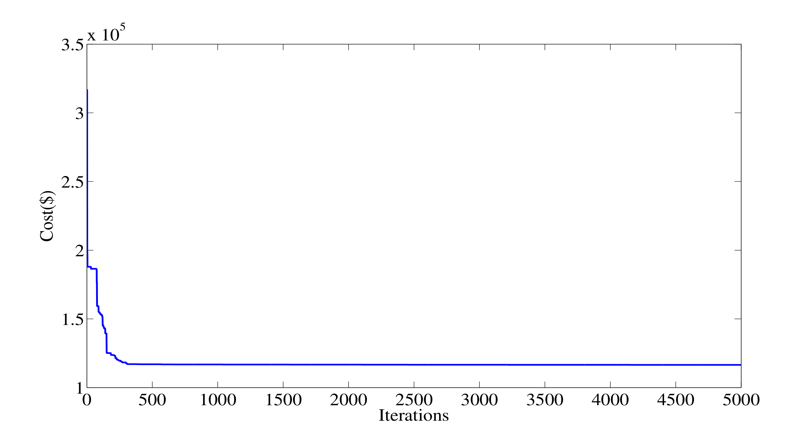
- The algorithm converges in relatively small number of iterations. This means that the algorithm has a good converge speed which enables it to be used in large systems.
- In test system I, the obtained value for the objective function is less than the average value in 66% of the trial runs. This is 54% for test system II and 56% for test system III, which means that the proposed algorithm is able to attain solutions lower than the mean value, in more than half of the trials.
- The obtained results are also feasible which indicates that the algorithm has the capability of attaining solutions which are both optimal and feasible.
Author Contributions
Funding
Conflicts of Interest
Parameters
The electric power load of the system []. | |
The heat load of the system []. | |
The electric power loss of the transmission system []. | |
Maximum/minimum generated electric power of eth power-only unit []. | |
Maximum/minimum generated heat of hth boiler []. | |
Maximum power output of cth CHP unit in when generating MWth heat. | |
Minimum power output of cth CHP unit in when generating MWth heat. | |
Maximum heat output of cth CHP unit in when generating MW power. | |
Minimum heat output of cth CHP unit in when generating MW power. | |
Quadratic cost coefficient of power-only unit e []. | |
Linear cost coefficient of power-only unit e [$/MWh]. | |
No-load cost coefficient of power-only unit e [$/h]. | |
Magnitude of sinusoidal term in cost function of power-only unit e [$/h]. | |
Frequency of sinusoidal term in cost function of power-only unit e [rad/MWh]. | |
Quadratic cost coefficient of heat-only unit h. | |
Linear cost coefficient of heat-only unit h [$/(MWth)h]. | |
No-load cost coefficient of heat-only unit h [$/h]. | |
Quadratic cost coefficient of CHP unit c []. | |
Linear cost coefficient of CHP unit c [$/MWh]. | |
No-load cost coefficient of CHP unit c []. | |
Quadratic cost coefficient of CHP unit c []. | |
Linear cost coefficient of CHP unit c [$/(MWth)h]. | |
Quadratic cost coefficient of CHP unit c []. |
Continuous Variables
Power output of ith power-only unit at time t. | |
Power output of jth CHP unit at time t. | |
Heat output of jth CHP unit at time t. | |
Heat output of kth heat-only unit at time t. |
Functions
Cost function of e-th power-only unit. | |
Cost function of c-th CHP unit. | |
Cost function of h-th heat-only unit. |
References
- Kazda, K.; Li, X. A Critical Review of the Modeling and Optimization of Combined Heat and Power Dispatch. Processes 2020, 8, 441. [Google Scholar] [CrossRef]
- Alipour, M.; Mohammadi-Ivatloo, B.; Zare, K. Stochastic risk-constrained short-term scheduling of industrial cogeneration systems in the presence of demand response programs. Appl. Energy 2014, 136, 393–404. [Google Scholar] [CrossRef]
- Nazari-Heris, M.; Mohammadi-Ivatloo, B.; Asadi, S.; Geem, Z.W. Large-scale combined heat and power economic dispatch using a novel multi-player harmony search method. Appl. Therm. Eng. 2019, 154, 493–504. [Google Scholar] [CrossRef]
- Rong, A.; Hakonen, H.; Lahdelma, R. An efficient linear model and optimisation algorithm for multi-site combined heat and power production. Eur. J. Oper. Res. 2006, 168, 612–632. [Google Scholar] [CrossRef]
- Ghorbani, N. Combined heat and power economic dispatch using exchange market algorithm. Int. J. Electr. Power Energy Syst. 2016, 82, 58–66. [Google Scholar] [CrossRef]
- Rooijers, F.; van Amerongen, R. Static economic dispatch for co-generation systems. Power Syst. IEEE Trans. 1994, 9, 1392–1398. [Google Scholar] [CrossRef]
- Guo, T.; Henwood, M.I.; van Ooijen, M. An algorithm for heat and power dispatch. IEEE Trans. Power Syst. 1996, 11, 1778–1784. [Google Scholar] [CrossRef]
- Sashirekha, A.; Pasupuleti, J.; Moin, N.; Tan, C. Combined heat and power (CHP) economic dispatch solved using Lagrangian relaxation with surrogate subgradient multiplier updates. Int. J. Electr. Power Energy Syst. 2013, 44, 421–430. [Google Scholar] [CrossRef]
- Jubril, A.; Adediji, A.; Olaniyan, O. Solving the Combined Heat and Power Dispatch Problem: A Semi-definite Programming Approach. Electr. Power Components Syst. 2012, 40, 1362–1376. [Google Scholar] [CrossRef]
- Rao, P. Combined heat and power economic dispatch: A direct solution. Electr. Power Compon. Syst. 2006, 34, 1043–1056. [Google Scholar] [CrossRef]
- Geem, Z.W.; Cho, Y.H. Handling non-convex heat-power feasible region in combined heat and power economic dispatch. Int. J. Electr. Power Energy Syst. 2012, 34, 171–173. [Google Scholar] [CrossRef]
- Subbaraj, P.; Rengaraj, R.; Salivahanan, S. Enhancement of combined heat and power economic dispatch using self adaptive real-coded genetic algorithm. Appl. Energy 2009, 86, 915–921. [Google Scholar] [CrossRef]
- Gopalakrishnan, H.; Kosanovic, D. Operational planning of combined heat and power plants through genetic algorithms for mixed 0–1 nonlinear programming. Comput. Oper. Res. 2015, 56, 51–67. [Google Scholar] [CrossRef]
- Ramesh, V.; Jayabaratchi, T.; Shrivastava, N.; Baska, A. A Novel Selective Particle Swarm Optimization Approach for Combined Heat and Power Economic Dispatch. Electr. Power Compon. Syst. 2009, 37, 1231–1240. [Google Scholar] [CrossRef]
- Mohammadi-Ivatloo, B.; Moradi-Dalvand, M.; Rabiee, A. Combined heat and power economic dispatch problem solution using particle swarm optimization with time varying acceleration coefficients. Electr. Power Syst. Res. 2013, 95, 9–18. [Google Scholar] [CrossRef]
- Wang, L.; Singh, C. Stochastic combined heat and power dispatch based on multi-objective particle swarm optimization. Int. J. Electr. Power Energy Syst. 2008, 30, 226–234. [Google Scholar] [CrossRef]
- Khorram, E.; Jaberipour, M. Harmony search algorithm for solving combined heat and power economic dispatch problems. Energy Convers. Manag. 2011, 52, 1550–1554. [Google Scholar] [CrossRef]
- Song, Y.; Chou, C.; Stonham, T. Combined heat and power economic dispatch by improved ant colony search algorithm. Electr. Power Syst. Res. 1999, 52, 115–121. [Google Scholar] [CrossRef]
- Niknam, T.; Azizipanah-Abarghooee, R.; Roosta, A.; Amiri, B. A new multi-objective reserve constrained combined heat and power dynamic economic emission dispatch. Energy 2012, 42, 530–545. [Google Scholar] [CrossRef]
- Chen, C.; Lee, T.; Jan, R.; Lu, C. A novel direct search approach for combined heat and power dispatch. Int. J. Electr. Power Energy Syst. 2012, 43, 766–773. [Google Scholar] [CrossRef]
- Basu, M. Artificial immune system for combined heat and power economic dispatch. Int. J. Electr. Power Energy Syst. 2012, 43, 1–5. [Google Scholar] [CrossRef]
- Basu, M. Bee colony optimization for combined heat and power economic dispatch. Expert Syst. Appl. 2011, 38, 13527–13531. [Google Scholar] [CrossRef]
- Basu, M. Combined Heat and Power Economic Dispatch by Using Differential Evolution. Electr. Power Compon. Syst. 2010, 38, 996–1004. [Google Scholar] [CrossRef]
- Dieu, V.; Ongsakul, W. Augmented LagrangeHopfield Network for Economic Load Dispatch with Combined Heat and Power. Electr. Power Compon. Syst. 2009, 37, 1289–1304. [Google Scholar] [CrossRef]
- Piperagkas, G.; Anastasiadis, A.; Hatziargyriou, N. Stochastic PSO-based heat and power dispatch under environmental constraints incorporating CHP and wind power units. Electr. Power Syst. Res. 2011, 81, 209–218. [Google Scholar] [CrossRef]
- Nazari-Heris, M.; Mohammadi-Ivatloo, B.; Gharehpetian, G. A comprehensive review of heuristic optimization algorithms for optimal combined heat and power dispatch from economic and environmental perspectives. Renew. Sustain. Energy Rev. 2018, 81, 2128–2143. [Google Scholar] [CrossRef]
- Neumaier, A.; Shcherbina, O.; Huyer, W.; Vinkó, T. A comparison of complete global optimization solvers. Math. Program. 2005, 103, 335–356. [Google Scholar] [CrossRef]
- Bonami, P.; Biegler, L.T.; Conn, A.R.; Cornuéjols, G.; Grossmann, I.E.; Laird, C.D.; Lee, J.; Lodi, A.; Margot, F.; Sawaya, N.; et al. An algorithmic framework for convex mixed integer nonlinear programs. Discret. Optim. 2008, 5, 186–204. [Google Scholar] [CrossRef]
- Klanšek, U.; Pšunder, M. Solving the nonlinear transportation problem by global optimization. Transport 2010, 25, 314–324. [Google Scholar] [CrossRef]
- Lastusilta, T.; Bussieck, M.R.; Westerlund, T. An experimental study of the GAMS/AlphaECP MINLP solver. Ind. Eng. Chem. Res. 2009, 48, 7337–7345. [Google Scholar] [CrossRef]
- Klanšek, U. A comparison between MILP and MINLP approaches to optimal solution of Nonlinear Discrete Transportation Problem. Transport 2015, 30, 135–144. [Google Scholar] [CrossRef]
- Karaboga, D.; Basturk, B. On the performance of artificial bee colony (ABC) algorithm. Appl. Soft Comput. 2008, 8, 687–697. [Google Scholar] [CrossRef]
- Mohammadi-Ivatloo, B.; Rabiee, A.; Soroudi, A. Nonconvex Dynamic Economic Power Dispatch Problems Solution Using Hybrid Immune-Genetic Algorithm. IEEE Syst. J. 2013, 7, 777–785. [Google Scholar] [CrossRef]
- Alipour, M.; Zare, K.; Mohammadi-Ivatloo, B. Short-term scheduling of combined heat and power generation units in the presence of demand response programs. Energy 2014, 71, 289–301. [Google Scholar] [CrossRef]
- Alipour, M.; Mohammadi-Ivatloo, B.; Zare, K. Stochastic Scheduling of Renewable and CHP-Based Microgrids. Ind. Inform. IEEE Trans. 2015, 11, 1049–1058. [Google Scholar] [CrossRef]
- Akay, B.; Karaboga, D. A modified artificial bee colony algorithm for real-parameter optimization. Inf. Sci. 2012, 192, 120–142. [Google Scholar] [CrossRef]
- Uzlu, E.; Akpınar, A.; Özturk, H.T.; Nacar, S.; Kankal, M. Estimates of hydroelectric generation using neural networks with the artificial bee colony algorithm for Turkey. Energy 2014, 69, 638–647. [Google Scholar] [CrossRef]
- Oliva, D.; Cuevas, E.; Pajares, G. Parameter identification of solar cells using artificial bee colony optimization. Energy 2014, 72, 93–102. [Google Scholar] [CrossRef]
- Gao, W.F.; Liu, S.Y. A modified artificial bee colony algorithm. Comput. Oper. Res. 2012, 39, 687–697. [Google Scholar] [CrossRef]
- Zhu, G.; Kwong, S. Gbest-guided artificial bee colony algorithm for numerical function optimization. Appl. Math. Comput. 2010, 217, 3166–3173. [Google Scholar] [CrossRef]
- He, S.; Wu, Q.; Saunders, J. Group search optimizer: An optimization algorithm inspired by animal searching behavior. Evol. Comput. IEEE Trans. 2009, 13, 973–990. [Google Scholar] [CrossRef]
- Shi, B.; Yan, L.X.; Wu, W. Multi-objective optimization for combined heat and power economic dispatch with power transmission loss and emission reduction. Energy 2013, 56, 135–143. [Google Scholar] [CrossRef]
- Roy, P.K.; Paul, C.; Sultana, S. Oppositional teaching learning based optimization approach for combined heat and power dispatch. Int. J. Electr. Power Energy Syst. 2014, 57, 392–403. [Google Scholar] [CrossRef]
- Basu, M. Combined heat and power economic emission dispatch using nondominated sorting genetic algorithm-II. Int. J. Electr. Power Energy Syst. 2013, 53, 135–141. [Google Scholar] [CrossRef]
- Jayakumar, N.; Subramanian, S.; Ganesan, S.; Elanchezhian, E. Grey wolf optimization for combined heat and power dispatch with cogeneration systems. Int. J. Electr. Power Energy Syst. 2016, 74, 252–264. [Google Scholar] [CrossRef]
- Mohammadi-Ivatloo, B.; Rabiee, A.; Soroudi, A.; Ehsan, M. Iteration PSO with time varying acceleration coefficients for solving non-convex economic dispatch problems. Int. J. Electr. Power Energy Syst. 2012, 42, 508–516. [Google Scholar] [CrossRef]
- Niu, Q.; Zhang, H.; Wang, X.; Li, K.; Irwin, G.W. A hybrid harmony search with arithmetic crossover operation for economic dispatch. Int. J. Electr. Power Energy Syst. 2014, 62, 237–257. [Google Scholar] [CrossRef]
- Hagh, M.T.; Teimourzadeh, S.; Alipour, M.; Aliasghary, P. Improved group search optimization method for solving CHPED in large scale power systems. Energy Convers. Manag. 2014, 80, 446–456. [Google Scholar] [CrossRef]


| Name | Formula | D (Problem Dimension) | Search Space | Global Minimum |
|---|---|---|---|---|
| Schaffer [39] | 30 | 0 | ||
| Rosenbrock [39] | 30 | 0 | ||
| Sphere [39] | 30 | 0 | ||
| Griewank [39] | 30 | 0 | ||
| Rastrigin [40] | 30 | 0 | ||
| Ackly [39] | 30 | 0 |
| Benchmark Function | ABC [40] | GABC [40] | MABC [39] | Proposed | |||||
|---|---|---|---|---|---|---|---|---|---|
| Number | Name | Mean | SD | Mean | SD | Mean | SD | Mean | SD |
| [39] | Schaffer | 4.47 × 10 | 2.22 × 10 | 2.81 × 10 | 9.12 × 10 | 2.56 × 10 | 4.65 × 10 | 2.12 × 10 | 2.23 × 10 |
| [39] | Rosenbrock | 3.65 × 10 | 5.04 × 10 | 7.93 × 10 | 1.36 × 10 | 1.73 × 10 | 1.61 × 10 | 1.05 × 10 | 1.45 × 10 |
| [39] | Sphere | 6.38 × 10 | 1.20 × 10 | 4.17 × 10 | 7.36 × 10 | 9.43 × 10 | 6.67 × 10 | 3.21 × 10 | 1.30 × 10 |
| [39] | Griewank | 1.27 × 10 | 1.46 × 10 | 2.96 × 10 | 4.99 × 10 | 0.00 | 0.00 | 0.00 | 0.00 |
| [40] | Rastrigin | 1.35 × 10 | 7.97 × 10 | 1.32 × 10 | 2.44 × 10 | 0.00 | 0.00 | 0.00 | 0.00 |
| [39] | Ackly | 4.70 × 10 | 5.95 × 10 | 3.21 × 10 | 3.25 × 10 | 2.98 × 10 | 2.26 × 10 | 2.87 × 10 | 3.65 × 10 |
| # | GSO [41] | GA [41] | PSO [41] | EP [41] | ES [41] | ABC [36] | MABC [39] | Proposed |
|---|---|---|---|---|---|---|---|---|
| 1.82 × 10 | 3.70 × 10 | 1.81 × 10 | 2.84 × 10 | 1.58 × 10 | 1.35 × 10 | 8.35 × 10 | 0 | |
| 98.9 | 121.3 | 427.1 | 383.3 | 583.2 | 6.82 × 10 | 1.04 × 10 | 0 | |
| 1.35 × 10 | 6.24 × 10 | 3.95 × 10 | 2.95 × 10 | 9.62 × 10 | 7.52 × 10 | 9.62 × 10 | 8.93 × 10 |
| ABC [36] | MABC [39] | Proposed | ||||
|---|---|---|---|---|---|---|
| # | Best | Worst | Best | Worst | Best | Worst |
| 0 | 6.46 × 10 | 7.55 × 10 | 9.44 × 10 | 0 | 0 | |
| 0 | 1.14 × 10 | 4.27 × 10 | 5.20 × 10 | 0 | 0 | |
| 5.33 × 10 | 1.10 × 10 | 7.80 × 10 | 1.08 × 10 | 6.82 × 10 | 1.10 × 10 | |
| Test System # | SN | Limit | |
|---|---|---|---|
| I | 100 | 50 | 300 |
| II | 200 | 50 | 2000 |
| III | 200 | 100 | 5000 |
| Power Only Units | |||||||
|---|---|---|---|---|---|---|---|
| Unit | |||||||
| 1 | 0.008 | 2 | 25 | 100 | 0.042 | 10 | 75 |
| 2 | 0.003 | 1.8 | 60 | 140 | 0.04 | 20 | 125 |
| 3 | 0.0012 | 2.1 | 100 | 160 | 0.038 | 30 | 175 |
| 4 | 0.001 | 2 | 120 | 180 | 0.037 | 40 | 250 |
| CHP Units | |||||||
| feasible region coordinates [] | |||||||
| 5 | 0.0345 | 14.5 | 2650 | 0.03 | 4.2 | 0.031 | [98.8,0], [81,104.8], [215,180], [247,0] |
| 6 | 0.0435 | 36 | 1250 | 0.027 | 0.6 | 0.11 | [44,0], [44,15.9],[40,75],[110.2,135.6], [125.8,32.4],[125.8,0] |
| Heat Only Units | |||||||
| 7 | 0.038 | 2.0109 | 950 | 0 | 2695.20 |
| Control Variable | LCA [42] | OTLBO [43] | TLBO [43] | CPSO [15] | TVAC-PSO [15] | Proposed |
|---|---|---|---|---|---|---|
| 44.2812 | 45.8860 | 45.2660 | 75.0000 | 47.3383 | 45.8514 | |
| 98.5446 | 98.5398 | 98.5479 | 112.3800 | 98.5398 | 98.5388 | |
| 112.7192 | 112.6741 | 112.6786 | 30.0000 | 112.6735 | 112.6734 | |
| 211.4443 | 209.8141 | 209.8284 | 250.0000 | 209.8158 | 209.8169 | |
| 93.7494 | 93.8249 | 94.4121 | 93.2701 | 92.3718 | 93.8594 | |
| 40.0000 | 40.0002 | 40.0062 | 40.1585 | 40.0000 | 40.0000 | |
| 29.7358 | 29.2914 | 25.8365 | 32.5655 | 37.8467 | 29.0616 | |
| 74.5000 | 75.0002 | 74.9970 | 72.6738 | 74.9999 | 74.9839 | |
| 45.2641 | 45.7084 | 49.1666 | 44.7606 | 37.1532 | 45.9542 | |
| Minimum Cost ($/h) | 10,104.38 | 10,094.3529 | 10,094.8384 | 10,325.3339 | 10,100.3164 | 10,094.2718 |
| Average Cost ($/h) | NA | 10,099.4057 | 10,114.1539 | NA | NA | 10,095.4446 |
| Maximum Cost ($/h) | NA | 10,106.8314 | 10,133.6130 | NA | NA | 10,100.9445 |
| CPU time (s) | NA | 3.06 | 2.86 | 3.29 | 3.25 | 2.21 |
| Control Variable | RCGA [44] | GWO [45] | Proposed (IABC) | |
|---|---|---|---|---|
| 74.5357 | 52.8074 | 45.2848 | ||
| 99.3518 | 98.5398 | 98.5507 | ||
| 174.7196 | 112.6735 | 112.6845 | ||
| 211.017 | 209.8158 | 209.8439 | ||
| 100.9363 | 93.8115 | 93.8194 | ||
| 44.1036 | 40 | 40.0000 | ||
| 24.3678 | 29.3704 | 29.3226 | ||
| 72.527 | 75 | 74.9944 | ||
| 53.1052 | 29.3704 | 45.6832 | ||
| Minimum Cost ($/h) | 10,712.86 | 10,111.24 | 10,092.9593 | |
| Average Cost ($/h) | NA | 10,194.41 | 10,152.5012 | |
| Maximuum Cost ($/h) | NA | 10,452.12 | 11,547.5437 | |
| CPU time (s) | 20.3438 | 5.2618 | 2.21 |
| Control Variable | EP [22] | BCO [22] | AIS [21] | PSO [22] | DE [23] | RCGA [22] | Proposed |
|---|---|---|---|---|---|---|---|
| 61.361 | 43.9457 | 50.1325 | 18.4626 | 44.2118 | 74.6834 | 52.5848 | |
| 95.1205 | 98.5888 | 95.5552 | 124.2602 | 98.5383 | 97.9578 | 98.5685 | |
| 99.9427 | 112.9320 | 110.7515 | 112.7794 | 112.6913 | 167.2308 | 112.7003 | |
| 208.7319 | 209.7719 | 208.7688 | 209.8158 | 209.7741 | 124.9079 | 209.8723 | |
| 98.8000 | 98.8000 | 98.8000 | 98.8140 | 98.8217 | 98.8008 | 93.8212 | |
| 44.0000 | 44.0000 | 44.0000 | 44.0107 | 44.0000 | 44.0001 | 40.0000 | |
| 18.0713 | 12.0974 | 19.4242 | 57.9236 | 12.5379 | 58.0965 | 29.3057 | |
| 77.5548 | 78.0236 | 77.0777 | 32.7603 | 78.3481 | 32.4116 | 74.9573 | |
| 54.3739 | 59.879 | 53.4981 | 59.3161 | 59.1139 | 59.4919 | 45.7375 | |
| Minimum Cost ($/h) | 10,390.0000 | 10,317.0000 | 10,355.0000 | 10,613.0000 | 10,317.0000 | 10,667.0000 | 10,111.8592 |
| Average Cost ($/h) | NA | NA | NA | NA | NA | NA | 10,656.4161 |
| Maximum Cost ($/h) | NA | NA | NA | NA | NA | NA | 13,638.7295 |
| CPU time (s) | 5.27 | 5.16 | 5.29 | 5.38 | 5.26 | 6.47 | 2.21 |
| Power Only Units | |||||||
|---|---|---|---|---|---|---|---|
| Unit | |||||||
| 1 | 0.00028 | 8.1 | 550 | 300 | 0.035 | 0 | 680 |
| 2 | 0.00056 | 8.1 | 309 | 200 | 0.042 | 0 | 360 |
| 3 | 0.00056 | 8.1 | 309 | 200 | 0.042 | 0 | 360 |
| 4 | 0.00324 | 7.74 | 240 | 150 | 0.063 | 60 | 180 |
| 5 | 0.00324 | 7.74 | 240 | 150 | 0.063 | 60 | 180 |
| 6 | 0.00324 | 7.74 | 240 | 150 | 0.063 | 60 | 180 |
| 7 | 0.00324 | 7.74 | 240 | 150 | 0.063 | 60 | 180 |
| 8 | 0.00324 | 7.74 | 240 | 150 | 0.063 | 60 | 180 |
| 9 | 0.00324 | 7.74 | 240 | 150 | 0.063 | 60 | 180 |
| 10 | 0.00284 | 8.6 | 126 | 100 | 0.084 | 40 | 120 |
| 11 | 0.00284 | 8.6 | 126 | 100 | 0.084 | 40 | 120 |
| 12 | 0.00284 | 8.6 | 126 | 100 | 0.084 | 55 | 120 |
| 13 | 0.00284 | 8.6 | 126 | 100 | 0.084 | 55 | 120 |
| CHP Units | |||||||
| feasible region coordinates [] | |||||||
| 14 | 0.0345 | 14.5 | 2650 | 0.03 | 4.2 | 0.031 | [98.8,0], [81,104.8], [215,180], [247,0] |
| 15 | 0.0435 | 36 | 1250 | 0.027 | 0.6 | 0.011 | [44,0], [44,15.9],[40,75],[110.2,135.6], [125.8,32.4],[125.8,0] |
| 16 | 0.0345 | 14.5 | 2650 | 0.03 | 4.2 | 0.031 | [98.8,0], [81,104.8], [215,180], [247,0] |
| 17 | 0.0435 | 36 | 1250 | 0.027 | 0.6 | 0.011 | [44,0], [44,15.9],[40,75],[110.2,135.6], [125.8,32.4],[125.8,0] |
| 18 | 0.1035 | 34.5 | 2650 | 0.025 | 2.203 | 0.051 | [20,0],[10,40], [45,55],[60,0] |
| 19 | 0.072 | 20 | 1565 | 0.02 | 2.34 | 0.04 | [35,0],[35,20],[ 90,45],[90,25], [105,0] |
| Heat Only Units | |||||||
| 20 | 0.038 | 2.0109 | 950 | 0 | 2695.20 | ||
| 21 | 0.038 | 2.0109 | 950 | 0 | 60 | ||
| 22 | 0.038 | 2.0109 | 950 | 0 | 60 | ||
| 23 | 0.052 | 3.0651 | 480 | 0 | 120 | ||
| 24 | 0.052 | 3.0651 | 480 | 0 | 120 |
| Control Variable | TLBO [43] | TVAC-PSO [15] | ACHS [47] | OTLBO [43] | CPSO [15] | GSO [48] | IGSO [48] | GWO [45] | Proposed (IABC) |
|---|---|---|---|---|---|---|---|---|---|
| 538.5656 | 538.5656 | 628.3185 | 538.5656 | 680 | 627.7455 | 628.152 | 538.584 | 628.3185 | |
| 299.2123 | 299.2123 | 299.1992 | 299.2123 | 0 | 76.2285 | 299.4778 | 299.3423 | 299.1993 | |
| 299.122 | 299.122 | 299.199 | 299.122 | 0 | 299.5794 | 154.5535 | 299.3423 | 299.1993 | |
| 109.992 | 109.992 | 109.8665 | 109.992 | 180 | 159.4386 | 60.846 | 109.9653 | 109.8665 | |
| 109.9545 | 109.9545 | 109.8665 | 109.9545 | 180 | 61.2378 | 103.8538 | 109.9653 | 109.8666 | |
| 110.4042 | 110.4042 | 60 | 110.4042 | 180 | 60 | 110.0552 | 109.9653 | 60 | |
| 109.8045 | 109.8045 | 109.8665 | 109.8045 | 180 | 157.1503 | 159.0773 | 109.9653 | 109.8666 | |
| 109.6862 | 109.6862 | 109.8665 | 109.6862 | 180 | 107.2654 | 109.8258 | 109.9653 | 109.8665 | |
| 109.8992 | 109.8992 | 109.8665 | 109.8992 | 180 | 110.1816 | 159.992 | 109.9653 | 109.8665 | |
| 77.3992 | 77.3992 | 40 | 77.3992 | 50.5304 | 113.9894 | 41.103 | 77.6223 | 40 | |
| 77.8364 | 77.8364 | 76.9505 | 77.8364 | 50.5304 | 79.7755 | 77.7055 | 77.6223 | 76.9498 | |
| 55.2225 | 55.2225 | 55 | 55.2225 | 55 | 91.1668 | 94.9768 | 55 | 55 | |
| 55.0861 | 55.0861 | 55 | 55.0861 | 55 | 115.6511 | 55.7143 | 55 | 55 | |
| 81.7524 | 81.7524 | 81 | 81.7524 | 117.4854 | 84.3133 | 83.9536 | 83.465 | 81 | |
| 41.7615 | 41.7615 | 40 | 41.7615 | 45.9281 | 40 | 40 | 40 | 40 | |
| 82.273 | 82.273 | 81 | 82.273 | 117.4854 | 81.1796 | 85.7133 | 82.7732 | 81 | |
| 40.5599 | 40.5599 | 40 | 40.5599 | 45.9281 | 40 | 40 | 40 | 40 | |
| 10.0002 | 10.0002 | 10 | 10.0002 | 10.0013 | 10 | 10 | 10 | 10 | |
| 31.4679 | 31.4679 | 35 | 31.4679 | 42.1109 | 35.097 | 35 | 31.4568 | 35 | |
| 105.2219 | 105.2219 | 104.8 | 105.2219 | 125.2754 | 106.6588 | 106.4569 | 106.0991 | 104.8 | |
| 76.5205 | 76.5205 | 75 | 76.5205 | 80.1175 | 74.998 | 74.998 | 75 | 75 | |
| 105.5142 | 105.5142 | 104.8 | 105.5142 | 125.2754 | 104.9002 | 107.4073 | 105.789 | 104.8 | |
| 75.4833 | 75.4833 | 75 | 75.4833 | 80.1174 | 74.998 | 74.998 | 75 | 75 | |
| 39.9999 | 39.9999 | 40 | 39.9999 | 40.0005 | 40 | 40 | 40 | 40 | |
| 18.3944 | 18.3944 | 20 | 18.3944 | 23.2322 | 19.7385 | 20 | 18.3782 | 20 | |
| 468.9043 | 468.9043 | 470.4 | 468.9043 | 415.9815 | 469.3368 | 466.2575 | 469.7337 | 470.3907 | |
| 59.9994 | 59.9994 | 60 | 59.9994 | 60 | 60 | 60 | 60 | 60 | |
| 59.9999 | 59.9999 | 60 | 59.9999 | 60 | 60 | 60 | 60 | 60 | |
| 119.9854 | 119.9854 | 120 | 119.9854 | 120 | 119.6511 | 120 | 120 | 120 | |
| 119.9768 | 119.9768 | 120 | 119.9768 | 120 | 119.7176 | 119.8823 | 120 | 120 | |
| Minimum cost | 58,006.9992 | 58,122.746 | 57,825.4368 | 57,856.2676 | 59,736.2635 | 58,225.745 | 58,049.0197 | 57,846.84 | 57,825.2594 |
| Maximum cost | 58,038.5273 | 58,359.552 | NA | 57,913.7731 | 60,076.6903 | 58,318.8792 | 58,219.1413 | 57,910.98 | 57,857.1058 |
| Mean cost | 58,006.9992 | 58,198.3106 | NA | 59,853.478 | 59,853.478 | 58,295.9243 | 58,156.5192 | 57,873.86 | 57,836.9224 |
| CPU time (s) | 5.67 | 52.25 | NA | 5.82 | 53.36 | 35.54 | 35.54 | 5.48 | 49.98 |
| Control Variable | TVAC-PSO [15] | CPSO [15] | GSO [48] | IGSO [48] | TLBO [43] | OLTBO [43] | Proposed |
|---|---|---|---|---|---|---|---|
| 538.5587 | 359.0392 | 627.5814 | 629.4952 | 538.5693 | 628.3199 | 628.3071 | |
| 75.134 | 74.5831 | 302.5046 | 151.9991 | 225.3021 | 225.3313 | 224.5321 | |
| 75.134 | 74.5831 | 225.3696 | 299.2996 | 229.9473 | 223.9653 | 224.6053 | |
| 140.6146 | 139.3803 | 178.6488 | 159.2254 | 159.1352 | 159.8516 | 159.7442 | |
| 140.6146 | 139.3803 | 178.2134 | 173.6004 | 160.0561 | 109.915 | 109.8049 | |
| 140.6146 | 139.3803 | 159.8844 | 93.4383 | 109.7821 | 159.7795 | 159.7348 | |
| 140.6146 | 139.3803 | 161.4173 | 160.773 | 159.6609 | 109.8946 | 109.9910 | |
| 140.6146 | 139.3803 | 108.776 | 159.351 | 159.6492 | 109.9321 | 110.0123 | |
| 140.6146 | 139.3803 | 109.0234 | 161.4184 | 109.966 | 159.9569 | 159.7589 | |
| 112.1998 | 74.7998 | 115.1364 | 115.2927 | 40.3726 | 40.897 | 40.0033 | |
| 112.1998 | 74.7998 | 114.2308 | 112.8994 | 77.5821 | 41.3115 | 40.0604 | |
| 74.7999 | 74.7998 | 107.2839 | 97.5394 | 92.2489 | 55.1748 | 55.1632 | |
| 74.7999 | 74.7998 | 93.0811 | 55 | 55.1755 | 92.4003 | 92.3016 | |
| 269.2794 | 679.881 | 0 | 0 | 448.6854 | 448.8359 | 359.0530 | |
| 299.1993 | 148.6585 | 223.7257 | 299.268 | 149.4238 | 225.7871 | 224.3763 | |
| 299.1993 | 148.6585 | 356.9056 | 225.4102 | 224.7173 | 75.46 | 74.8094 | |
| 140.3973 | 139.0809 | 109.2667 | 162.4605 | 109.9355 | 160.1192 | 159.6180 | |
| 140.3973 | 139.0809 | 160.4169 | 160.9664 | 159.9052 | 110.3532 | 109.7450 | |
| 140.3973 | 139.0809 | 109.6482 | 164.0177 | 159.7255 | 159.819 | 159.7410 | |
| 140.3973 | 139.0809 | 160.0005 | 168.4149 | 159.782 | 159.7765 | 159.8047 | |
| 140.3973 | 139.0809 | 174.5336 | 159.5402 | 60.0777 | 159.737 | 159.6745 | |
| 140.3973 | 139.0809 | 118.6394 | 110.8099 | 110.0689 | 160.1751 | 159.6378 | |
| 74.7998 | 74.7998 | 40.063 | 40.6399 | 77.6818 | 40.114 | 40.0053 | |
| 74.7998 | 74.7998 | 41.2253 | 114.3701 | 40.2707 | 40.3042 | 40.0109 | |
| 112.1997 | 112.1993 | 55 | 92.3275 | 92.4108 | 92.4149 | 92.1754 | |
| 112.1997 | 112.1993 | 92.0406 | 55 | 55.0956 | 92.5012 | 92.4037 | |
| 86.9119 | 92.8423 | 81.3512 | 82.1821 | 81.4882 | 85.9857 | 90.0393 | |
| 56.1027 | 98.7199 | 40 | 40 | 44.5478 | 98.5005 | 81.0528 | |
| 86.9119 | 92.8423 | 81.0383 | 81.089 | 81.056 | 81.7197 | 82.4319 | |
| 56.1027 | 98.7199 | 40 | 40.4281 | 91.6819 | 48.9055 | 81 | |
| 10.0031 | 10.0002 | 10 | 10.6913 | 10.548 | 10.0832 | 10 | |
| 35 | 56.7153 | 35.2736 | 35.0696 | 52.718 | 39.311 | 38.8071 | |
| 95.4799 | 109.1877 | 82.878 | 81 | 82.1522 | 82.0236 | 98.9499 | |
| 54.9235 | 65.6006 | 40 | 40.1014 | 52.0606 | 40.1105 | 81.0677 | |
| 95.4799 | 109.18 | 81 | 81.0922 | 82.7394 | 81.3039 | 98.9518 | |
| 54.9235 | 65.6006 | 40.3336 | 40.1056 | 45.7398 | 45.67 | 47.3001 | |
| 23.4981 | 10.6158 | 10.5087 | 10 | 10.0075 | 13.8709 | 10 | |
| 54.0882 | 60.5994 | 35 | 35.6838 | 30.0332 | 30.3881 | 35.3241 | |
| 108.1177 | 111.4458 | 104.9965 | 103.5903 | 105.0678 | 107.5951 | 109.8506 | |
| 88.9006 | 125.6898 | 74.998 | 74.998 | 78.9162 | 125.4997 | 110.4369 | |
| 108.1177 | 111.4458 | 104.8209 | 104.2548 | 104.827 | 105.1942 | 105.5403 | |
| 88.9006 | 125.6898 | 74.998 | 75.3686 | 119.6006 | 82.6853 | 110.3925 | |
| 40.0013 | 40.0001 | 40.001 | 40.0999 | 40.2345 | 40.0346 | 39.9999 | |
| 20 | 29.8706 | 19.2636 | 19.2943 | 28.0508 | 21.9568 | 21.7102 | |
| 112.926 | 120.6188 | 105.5564 | 104.8032 | 105.4339 | 105.3622 | 114.8715 | |
| 87.8827 | 97.0997 | 74.998 | 75.0858 | 85.40864 | 75.0938 | 110.4267 | |
| 112.926 | 120.6188 | 104.8032 | 104.8511 | 105.7694 | 104.9667 | 114.8542 | |
| 87.8827 | 97.0997 | 332.3293 | 75.086 | 79.9447 | 79.8936 | 81.2985 | |
| 45.7849 | 40.2639 | 39.5514 | 40 | 40.0001 | 41.6554 | 39.9999 | |
| 28.6765 | 31.6361 | 20 | 20.3111 | 17.7401 | 17.9018 | 20.1409 | |
| 433.9113 | 357.9456 | 486.4858 | 428.0157 | 394.616 | 445.0937 | 399.5313 | |
| 60 | 59.9916 | 60 | 59.5061 | 59.93 | 59.9967 | 60 | |
| 60 | 59.9916 | 60 | 59.9205 | 59.9578 | 59.9974 | 60 | |
| 120 | 120 | 118.7549 | 114.8048 | 118.5797 | 119.8834 | 120 | |
| 120 | 120 | 113.2371 | 117.9877 | 118.3425 | 119.5231 | 119.9999 | |
| 415.9741 | 370.6214 | 212.5981 | 535.65 | 480.6566 | 428.7605 | 400.9482 | |
| 60 | 59.9999 | 59.5362 | 60 | 59.9346 | 59.9957 | 60 | |
| 60 | 59.9999 | 59.9138 | 60 | 59.981 | 59.9638 | 60 | |
| 119.9989 | 119.9856 | 113.9272 | 107.7179 | 117.8207 | 119.5025 | 120 | |
| 119.9989 | 119.9856 | 119.2305 | 118.6434 | 119.1898 | 119.444 | 119.9999 | |
| Minimum cost | 117,824.8956 | 119,708.8818 | 117,824.896 | 112,320.4159 | 116,739.364 | 116,579.239 | 117,130.505 |
| Maximum cost | NA | NA | NA | NA | 116,756.0057 | 116,613.6505 | 117,182.5525 |
| Mean cost | NA | NA | NA | NA | 116,825.8223 | 116,649.4473 | 117,145.5397 |
| CPU time (s) | 89.63 | 93.32 | 70.65 | 70.65 | 10.38 | 10.93 | 89.51 |
| CHP Unit No. | TVAC-PSO [15] | CPSO [15] | OLTLBO [43] | TLBO [43] | GSO [48] | IGSO [48] | Proposed |
|---|---|---|---|---|---|---|---|
| 27 | 3 | 3 | 3 | 3 | 3 | 3 | 3 |
| 28 | 3 | 3 | 3 | 3 | 3 | 3 | 3 |
| 29 | 3 | 3 | 3 | 3 | × | 3 | 3 |
| 30 | 3 | 3 | 3 | 3 | 3 | 3 | 3 |
| 31 | 3 | 3 | 3 | 3 | 3 | 3 | 3 |
| 32 | 3 | 3 | 3 | 3 | 3 | 3 | 3 |
| 33 | 3 | 3 | 3 | 3 | 3 | 3 | 3 |
| 34 | 3 | 3 | 3 | 3 | 3 | 3 | 3 |
| 35 | 3 | 3 | 3 | 3 | 3 | 3 | 3 |
| 36 | 3 | 3 | 3 | 3 | 3 | × | 3 |
| 37 | 3 | 3 | 3 | 3 | 3 | 3 | 3 |
| 38 | 3 | 3 | × | × | 3 | 3 | 3 |
| Total Mismatch of Equations (6) and (8) | −2.00 × 10 | −3.00 × 10 | 0.064 | −1.00 × 10 | 6.23 × 10 |
© 2020 by the authors. Licensee MDPI, Basel, Switzerland. This article is an open access article distributed under the terms and conditions of the Creative Commons Attribution (CC BY) license (http://creativecommons.org/licenses/by/4.0/).
Share and Cite
Rabiee, A.; Jamadi, M.; Mohammadi-Ivatloo, B.; Ahmadian, A. Optimal Non-Convex Combined Heat and Power Economic Dispatch via Improved Artificial Bee Colony Algorithm. Processes 2020, 8, 1036. https://doi.org/10.3390/pr8091036
Rabiee A, Jamadi M, Mohammadi-Ivatloo B, Ahmadian A. Optimal Non-Convex Combined Heat and Power Economic Dispatch via Improved Artificial Bee Colony Algorithm. Processes. 2020; 8(9):1036. https://doi.org/10.3390/pr8091036
Chicago/Turabian StyleRabiee, Abbas, Mohammad Jamadi, Behnam Mohammadi-Ivatloo, and Ali Ahmadian. 2020. "Optimal Non-Convex Combined Heat and Power Economic Dispatch via Improved Artificial Bee Colony Algorithm" Processes 8, no. 9: 1036. https://doi.org/10.3390/pr8091036
APA StyleRabiee, A., Jamadi, M., Mohammadi-Ivatloo, B., & Ahmadian, A. (2020). Optimal Non-Convex Combined Heat and Power Economic Dispatch via Improved Artificial Bee Colony Algorithm. Processes, 8(9), 1036. https://doi.org/10.3390/pr8091036