1. Introduction
In many chemical, hydro-geological, petrochemical, and manufacturing processes the dynamic models take the mathematical form of partial differential equations (PDEs). One of these types of models is the Saint–Venant–Exner (SVE) equations, which consist of non-linear PDEs and are used to model the dynamics of a sediment-filled water canal with arbitrary values of the bottom slope, friction, porosity, and water-sediment interaction. Due to their nature, one of the crucial aspects of these distributed parameter systems is the complexity given by the infinite-dimensional system representation [
1,
2], which is a challenging factor when it comes to the controller/regulator design and realization.
The primary goal of a regulator is to drive the desired output of a system to behave exactly as demanded, and at the same time it needs to assure the stability of the closed-loop system. Using early lumping methods is the simplest way to design the controller for distributed parameter systems. In these methods, the PDEs are generally converted to sets of ordinary differential equations (ODEs), which allows the use of standard control methodology applicable to ODE systems. But, this also results in some mismatch between the dynamical properties of the original distributed parameter and the lumped parameter models, thus, affecting the controller [
3].
Another way to deal with distributed parameter processes is to exploit the infinite-dimensional characteristic of the system, and there are significant research efforts made to solve the regulator design problem for infinite-dimensional systems [
4,
5]. In [
6], the generalized geometric methods were introduced in the regulator design for the first-order hyperbolic PDEs, and the robust output regulation problems were considered in [
7,
8,
9], while taking into account infinite-dimensional exogenous systems (an independent system responsible for the generation of the tracking signal and/or disturbance). Specifically for the SVE model, there are several contributions that take into account the characteristics of the model. In [
10], the proportional and integral output feedback controllers were proposed by using the semigroup theory. The
optimization framework was applied in [
11] to design a controller considers the both water resource management and performance with respect to the users. And in [
12], a Lyapunov approach was used to obtain the control laws that stabilize the system considering full-state and output feedback.
More recently, in [
13], the exponential stabilization of this model was achieved by the backstepping design, also considering full-state and output feedback, where the design of an exponentially stable Luenberger observer was considered for state reconstruction. The PDE backstepping design has proved to be of valuable for the boundary stabilization of distributed parameter systems. Essentially, the technique consists of finding a suitable transformation that maps the closed-loop system into a stable target system. Due to the invertibility of the transformation, the original and the target system have equivalent stability [
14,
15]. Other applications and developments along this line include, for instance, the boundary observer based-control design for a hyperbolic PDE [
16], the boundary observer for a class of time-varying linear hyperbolic partial integral-differential equations (PIDEs) [
17], and control of general linear heterodirectional hyperbolic ODE–PDE–ODE systems [
18].
All the contributions mentioned above were developed in the continuous-time domain, but, as most modern and state-of-the-art controller realizations are digital and discrete, time discretization realizations need to be taken into account at the final design stage. Although some contributions addressed the stabilization of PDEs using backstepping with time sampled-data [
19,
20], these were made considering specific scalar equations and the design of a controller in the discrete-time setting was not the objective of these works. Traditional time discretization schemes (for instance, explicit or implicit Euler) could be used to obtain a discrete-time representation, but they have the disadvantage of reducing the accuracy of the discrete system representation as the sampling period increases [
21]. Moreover, the sampling may impact the overall model and closed-loop stability when the controller is implemented. Therefore, a different type of time discretization scheme, that provides a reliable transformation of a continuous linear infinite-dimensional system representation to a linear discrete-time infinite-dimensional needs to be considered. A discretization scheme that accounts for this design criteria is the Crank-Nicolson midpoint integration rule, which can be easily applied to infinite-dimensional systems [
22]. This type of discretization is also known as Cayley-Tustin time discretization, and it has been shown to preserve the intrinsic energy and dynamical characteristics of the linear distributed parameter system [
23] without the application of spatial discretization or/and model reduction.
The unstable linearized SVE model is considered in this manuscript. The PDE system is given as a system of first-order transport hyperbolic PDE equations, with in-domain and boundary coupling. Based on this system, a discrete-time output regulator design is presented and attains the following objectives: (1) ensures the stability by output feedback; (2) considers the stabilization of the problem in the discrete-time setting, obtained by the application of the Caley-Tustin time discretization; (3) achieves tracking of periodic and polynomial signals generated by an exosystem, which is ensured by the solution of the corresponding Sylvester output regulation equations. To properly design the discrete-time regulator, the relation between the discrete-time and continuous-time control is developed, such that the closed-loop stability and proper tracking of the discrete-time representation is assured if the controller design is known in the continuous-time.
The manuscript is organized as follows: in
Section 2, the SVE system model and its properties are introduced together with the exosystem and control objectives. In
Section 3, the system stabilization, observer design, and output regulation in the continuous-time setting are developed. In
Section 4, the Caley-Tustin time discretization is applied to the system, and the discrete regulator design is developed. The stability of the closed-loop system is shown. In
Section 5, the simulations results are presented and the regulator performance is discussed. Lastly, in
Section 6, the final remarks are made.
2. Problem Formulation
The Saint–Venant and Exner equations are used to describe the dynamics in a sediment-filled open channel with rectangular cross-section [
13]. Considering
to be the water depth,
as the water velocity and
as the depth of the sediment layer above the channel bottom, the dynamics of the system can be described as the equations below:
As shown in [
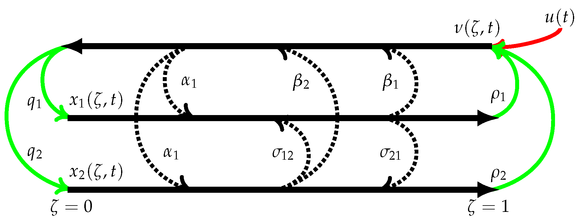
13], this system can be linearized around a steady-state and the Cardano-Vieta method can be applied to rewrite it in the characteristic form, which can be llustrated in
Figure 1.
This linearized system is given by the following coupled system of first-order hyperbolic partial differential equations, in the domain
, with
t representing time and
representing the dimensionless spatial variable:
With the following algebraic boundary conditions:
These linear hyperbolic PDEs represent the transport of
(a real Hilbert space);
,
and
are the system’s characteristics velocities;
for
and
,
,
and
are the parameters representing the in-domain interaction between the state variables; and
,
,
and
are parameters representing the interaction on the boundaries. All these parameters are obtained from the characteristic form of the SVE model [
13].
Usually, the openings of the gates located at the ends of the channel can be controlled to achieve the stabilization of the water level and flow rate. Thus,
(a real finite space), the system input, is considered to be control of the downstream gate, represented by the boundary actuation at
, shown in (
3). Measurements at the upstream (
) are considered to be the system measured output
and are used to reconstruct the states with a Luenberger observer. The system desired system output
is related to the properties of the water downstream. There are no direct measurements of this output and the regulator aim is to control it as desired. Thus, this system output should properly follow a predetermined pattern if the regulator is properly designed.
This system can be represented as an abstract differential equation:
where
A is a linear operator
,
B is the linear input operator
,
is the measured output operator
and
C is the desired output operator
.
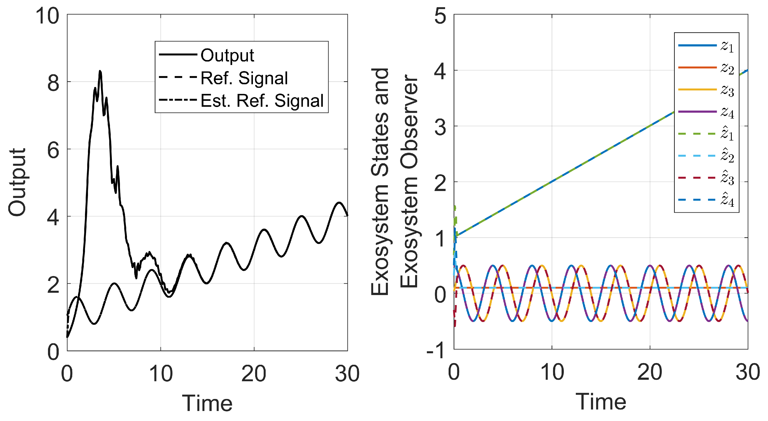
In this contribution, the goal is to achieve proper tracking of a reference signal, while maintaining the system stability. It is considered that the reference signal
to be tracked by the system output
is generated as the output of a known finite-dimensional exogenous system (also called exosystem), which is independent from the system (the exosystem affects the system dynamics, but not the other way around) and is defined as the following throughout this work:
where the matrix
gives the dynamics of the exosystem states and
Q is a matrix that gives the desired output tracking signal
.
Assumption 1. The reference signal consists of periodic and polynomial functions, such that the exosystem dynamics can be represented in the following form:notice that and are decoupled block matrices and it is assumed that each is unique. generates a polynomial signal and the size of () determines the polynomial degree. generates a linear combination of periodic function, where each is responsible for a function with different periodicity. Therefore, the size of will be , and it is an even number. Remark 1. The block matrix has all eigenvalues equal zero (i.e., ) with multiplicity equal to the size of the matrix. on the other hand has conjugated complex eigenvalues . Therefore, the spectra of S in Equation (5) is . Due to their structures, is a Jordan block, while is a diagonal block matrix and its eigenvectors are filled with zeros in all rows except in the ones that correspond to each . The elements in these rows will be and for the corresponding eigenvalues.
This exosystem will generate a linear combination of a polynomial (
from
) and periodic functions with frequencies
(
from
), and
and the initial conditions
are defined accordingly to match the desired tracking signal. Without loss of generality, one can extend the ensuing design to the case when the exosystem is infinite dimensional [
9].
In this contribution, an exosystem that generates a first-order polynomial in combination a periodic signal with one frequency is considered. Therefore, the desired reference signal (
) has a general form given by:
with:
The tracking error
is defined as the difference between the system output and the tracking signal:
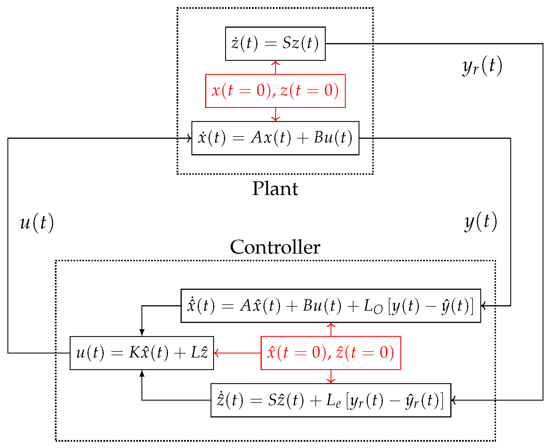
In the continuous-time setting the regulation problem can be defined as finding a regulator of the form:
where
is the linear feedback gain operator
that is used to stabilize the system and
L is the feedforward gain
that guarantees proper tracking of the desired signal. Therefore, the regulator should guarantee the following conditions:
The closed-loop system is exponentially stable;
For the closed-loop system, the tracking error ;
2.1. System Properties
2.1.1. Linearized System Stability
The system stability can be determined by the analysis of the eigenvalue problem , where are the eigenvector of the system, in this case given by , where are the eigenfunctions, and is the system eigenvalues.
Lemma 1. The eigenvalues of the system are given as the solution of the following non-linear equation:where are the elements of the exponential matrix given by , where V is a matrix with the system velocities and is the matrix with the in-domain coupling coefficients. Proof. The operator
A can be written as
, where
V is a matrix with the system velocities and
is a matrix with the in-domain coupling coefficients. For the particular system considered (given in Equation (
2)):
Therefore, the eigenvalue problem can be written as:
which has the following general solution:
with:
Finally, applying the boundary conditions of Equations (
3)–(
14) with the definition given in Equation (
15), the non-linear equation shown in Equation (
11) is obtained. ☐
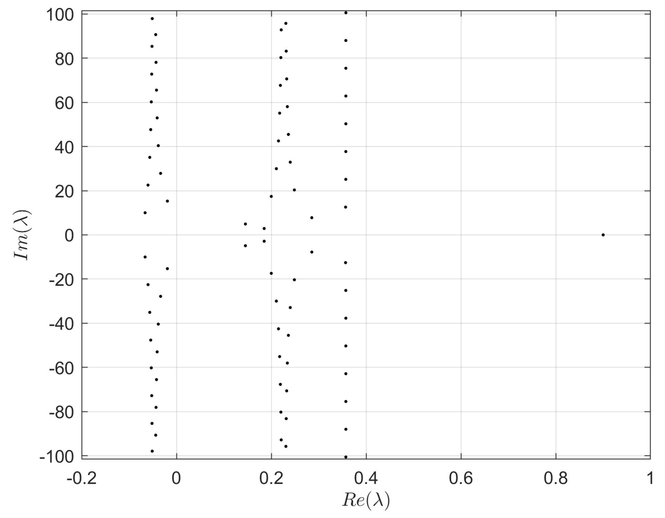
In this contribution, the system parameters as shown in
Table 1 are considered. For these values, the eigenvalue distribution is shown in
Figure 2. With the values considered, it is possible to conclude that the steady-state considered generates an unstable linearized system. Furthermore, it has an infinity number of unstable eigenvalues, which would not be easily stabilized with techniques generally used for linear finite systems, such as pole-placement.
2.1.2. Resolvent and Transfer Function
In this section, the system’s resolvent and transfer function are derived, as they will be used in the following sections. The resolvent is used to generate the discrete representation of the system, shown in
Section 4.1. The transfer function and the resolvent are also necessary to solve the Sylvester equations related to the output regulation problem, defined in
Section 3.2.
Lemma 2. The system resolvent is given by:with , with defined as in Equation (14) and is the same function given in Equation (11) (as expected, if ). and the system transfer function are: Proof. By applying Laplace Transform in the system defined by Equation (
4), the following system is obtained:
Using the fact that
gives the general solution as:
By applying the boundary conditions shown in Equation (
3), the general solution can be written as
where the operator
and the function
are the ones shown in Equations (
16) and (
17), respectively. ☐
4. Discrete Time Regulator Design
The discrete regulator design is considered in this section. It is necessary to find a control law for the discrete system that guarantees the closed-loop stability and proper output tracking.
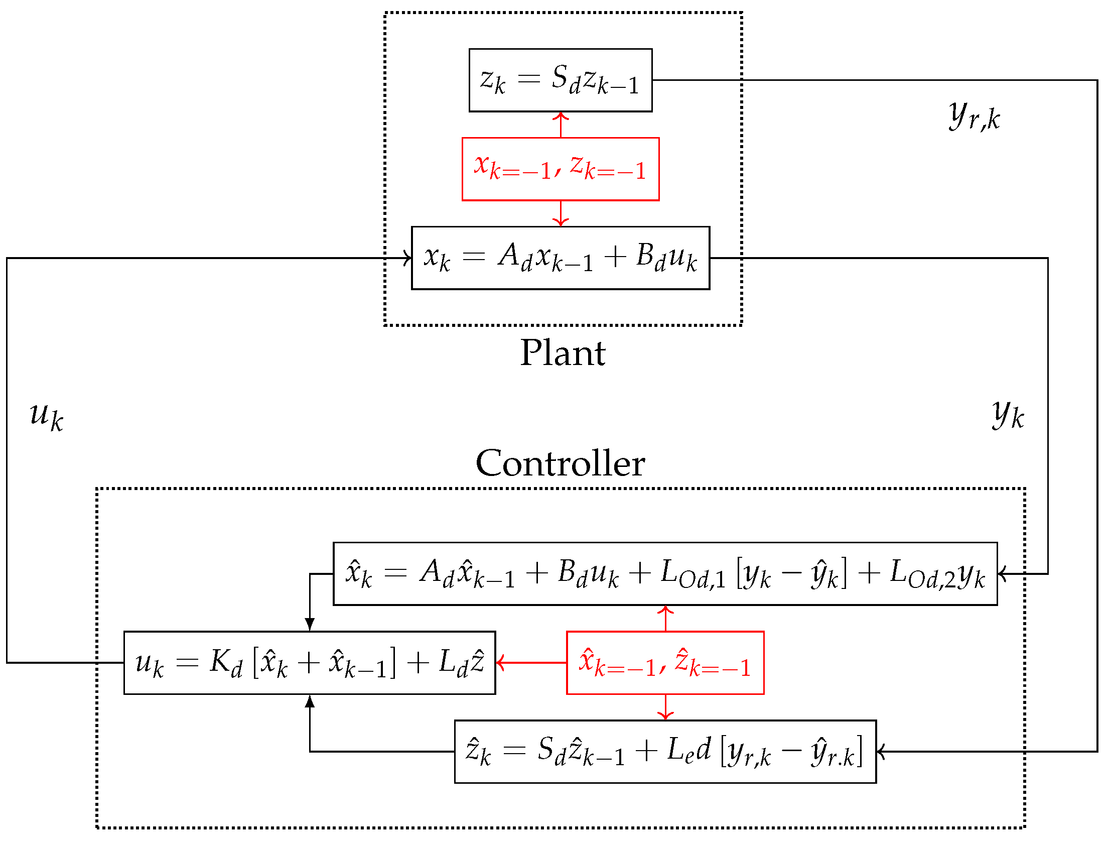
Figure 4 represents the closed-loop controller for the discrete setting. The closed-loop begins at the controller, where the initial condition for the system and exosystem observers (
and
) are used to calculate the first control action
. Then, the action is applied to the plant and the system measured output and the reference signal from the exosystem become available (
and
). These output are used to estimate the system and exosystem states in the observer (
and
). Finally, the estimates are used in the control law to calculate the next input (
) and the process is repeated.
The control law used to ensure the system stability and proper signal tracking is similar to the regulator equation shown in Equation (
10) for the continuous setting considering fullstate feedback:
where the first part of the right side of the control law represents the feedback control used to guarantee the system stability. The second part is responsible for the output tracking and
is a matrix that needs to be found to ensure proper output tracking.
The discrete output tracking error can be defined as:
Similar to the controller in the continuous time setting, the discrete regulator should guarantee:
The closed-loop system is stable;
For the closed-loop system, the tracking error ;
Before addressing the discrete regulator design, first the proper discrete representation of the system is considered.
4.1. Discrete Representation
Given the system defined in Equation (
4), one can apply a structure preserving time discretization of the dynamical system. By the application of Crank-Nicolson midpoint integration rule, and with the assumption of piecewise constant input within the sampled intervals, the Cayley-Tustin time discretization transformation is used. The obtained discrete system is represented as:
where
and
are the discrete time system operators and are given by:
and
is defined as the resolvent operator of the operator
A, which can be found in Equation (
16),
and
were defined in Equation (
17) for the specific system considered.
The operators given by Equation (
50) are all compact and well-defined and the issue of boundary (point) actuation or/and observation does not induce mathematical difficulties which are associated with the continuous counterparts, usually leading to unboundness of the boundary (point) actuation and/or observation.
Assumption 2. A small enough value of is used such that the discrete time representation of the system shown in Equation (49) is a good approximation of the open-loop system internal dynamics and input/output relation. Assumption 2 presumes there is a large enough
(small enough
) such that the discretization can be applied to unstable systems as well [
26] and is necessary for the development of the discrete regulator in the following sessions. For an unstable open-loop system, the following lemma gives an interval for which the discrete representation might be a good approximation of the system:
Lemma 8. In the case of an unstable system, the discrete system will not be a good discrete approximation of the system if , where .
Proof. For a stable system,
(all eigenvalues are negative), thus, as
and
,
exists for any value of
. For an unstable system,
, there will be at least one unstable eigenvalue with a positive real part. If this eigenvalue is real,
and
, if
. As the discrete operators shown in Equation (
49) depend on the resolvent,
will not result in a good discrete approximation. If the eigenvalue is complex, the Spectral Mapping Theorem can give an insight on the behavior of the discrete eigenvalue. If there exists a exact discrete representation of
A, it’s largest eigenvalue will be
, such that
and
. For the Cayley-Tustin transformation, this relation is given by
. If we calculate the modulus of these eigenvalues, we get:
As expected, if
,
and
. Taking the derivative with respect to
yields:
For the exact representation, the value of the discrete eigenvalues will decrease as increases (i.e., decreases). For the Cayley-Tustin transformation it is possible to see that the function will have an turning point at or . If , then and the functions have different responses, i.e., is increasing as increases, but will decrease past the turning point. Thus, will not generate a good discrete approximation of the system. ☐
Similar to the controller design in the continuous time setting, first the stabilization of the system in the discrete time setting given by Equations (
49) and (
50) is addressed.
4.2. Discrete System Stabilization
The design of the discrete regulator is considered in this section. First, it is shown in Lemma 9 that the discrete system can be stabilized.
Lemma 9. If K in the continuous time setting is able to stabilize the system, then there is a corresponding in the discrete time setting that ensures the discrete system stability with the control law: Proof. With the control law considered, the closed-loop discrete system is given by:
By using the definitions of the operators, the following relation can be achieved:
where the Woodbury identity was used to properly manipulate the expressions. The resulting operator is equivalent to the discrete operator obtained by applying the Cayley-Tustin time discretization in the closed-loop system obtained in
Section 3.1. Using the Cayley-Tustin transformation, the closed-loop system can be represented in the discrete setting as:
From [
27,
28], it was shown that a stable continuous operator generates a stable discrete operator, thus, if
is stable, then the discrete operator
is stable as well. Finally, if the control law proposed in Equation (
53) with
shown in Equation (
54), is used, then the closed-loop discrete operator is equivalent to the operator shown above and the discrete closed-loop system is stable as well (i.e.,
). ☐
With the proposed control law, the discrete closed-loop system is given as:
with:
4.3. Discrete Output Regulation
After achieving the system stabilization, it is possible to accomplish proper output tracking. First, the Cayley-Tustin time discretization is applied to the exosystem, such that the discrete time exosystem is given as:
with:
Then, it is necessary to find the discrete feedforward gain that is able to guarantee the proper tracking of the reference signal . This can be accomplished by solving the output regulator equations in the discrete-time setting.
4.3.1. Discrete Regulator Equations
In
Section 3.2, the regulation equations were solved in the continuous setting. In this section, the output regulation equations for the discrete time setting are derived. The following Lemma summarizes the results for the output tracking if the Cayley-Tustin time discretization is applied.
Lemma 10. If the Cayley-Tustin time discretization is considered, then the solution of the regulation equation (Sylvester equations) in the discrete setting is the same as in the continuous setting, i.e., , such that when proper tracking is achieved and it is the solution of the following Sylvester equations in the discrete-time setting: with the following relation between L and : Proof. The discrete control law that stabilizes the system and ensures the proper tracking of the discrete signal is given by: with the following relation between
L and
:
The discrete error is defined as
, which leads to:
and if the last term in brackets is equal zero, the error system becomes:
which is stable if
is stable. This yields the following Sylvester equation:
And the tracking error will be:
which gives the condition:
Lastly, the proof that
for the Cayley-Tustin time discretization is derived. First, the discrete Sylvester equation is considered and the definition of each operator is used:
And for the algebraic condition:
which is the same Sylvester equation and algebraic condition shown in the continuous-time setting (Equation (
29)), consequently,
. ☐
4.4. Discrete System Observer Design
The discrete observer design is considered in this section, as it was developed in
Section 3.3 in the continuous time setting. In the continuous setting (Equation (
43)), the observer does not have the same operator as the system (
is different from
A), thus, the discrete observer will also have different operators
and
when compared to the discrete system. Thus, the discrete system is observable as well and the discrete observer will take the following form:
where
and
have been defined previously. The other discrete operators are given as:
Notice that and have similar structure to , as the system measured output can be considered as an input to the observer as well.
Lemma 11. If the observer gains in the continuous time setting ( and ) are chosen such that is stable, then, the discrete observer given by Equation (72) and the operators defined in Equation (73) will be able to reconstruct the states of the discrete system (the discrete observer error - - decreases with time and eventually reaches the origin). Proof. To prove the observer states convergence to the system states, it is necessary to analyze the discrete observer error:
After some algebraic manipulation (shown in
Appendix C), the discrete error can be written as:
which is the discrete operator generated by
. Thus, if
is chosen such that
is stable, the discrete observer will be stable as well, as the Cayley-Tustin time discretization cannot map a stable continuous system to a unstable discrete one. ☐
4.5. Discrete Exosystem Observer Design
The discrete observer design for the exosystem is considered in this section using the discrete reference signal
. The following finite discrete observer is considered:
where
is the estimated exosystem state,
and
have been defined in
Section 4.3 (in Equation (
60)).
and
are defined as:
Lemma 12. If the exosystem observer gain in the continuous time setting () is chosen such that is stable, then, the discrete observer given by Equation (A23) and the operators defined in Equation (A24) will be able to reconstruct the states of the discrete exosystem.
Proof. To prove the exosystem observer convergence to the system states, the discrete error of the exosystem observer is analyzed:
After some algebraic manipulation (shown in
Appendix D), the discrete error can be written as:
which is the operator generated by the discrete representation of
. Thus, if
is chosen such that
is stable, the discrete observer will be stable as well. ☐
4.6. Finite-Time Discrete Exosystem Observer Design
The exosystem discrete dynamics is given by
and the reference signal is
. If the pair
is observable (which can be proved by the observability of
), then the exosystem states can be estimated in the discrete setting using the observability matrix:
where,
is the exosystem observability matrix in the discrete-time setting. Therefore, after
e time steps (and
e samples of
) it is possible to properly estimate
. For any instance before that, the discrete observer from
Section 4.5 can be used.
6. Conclusions
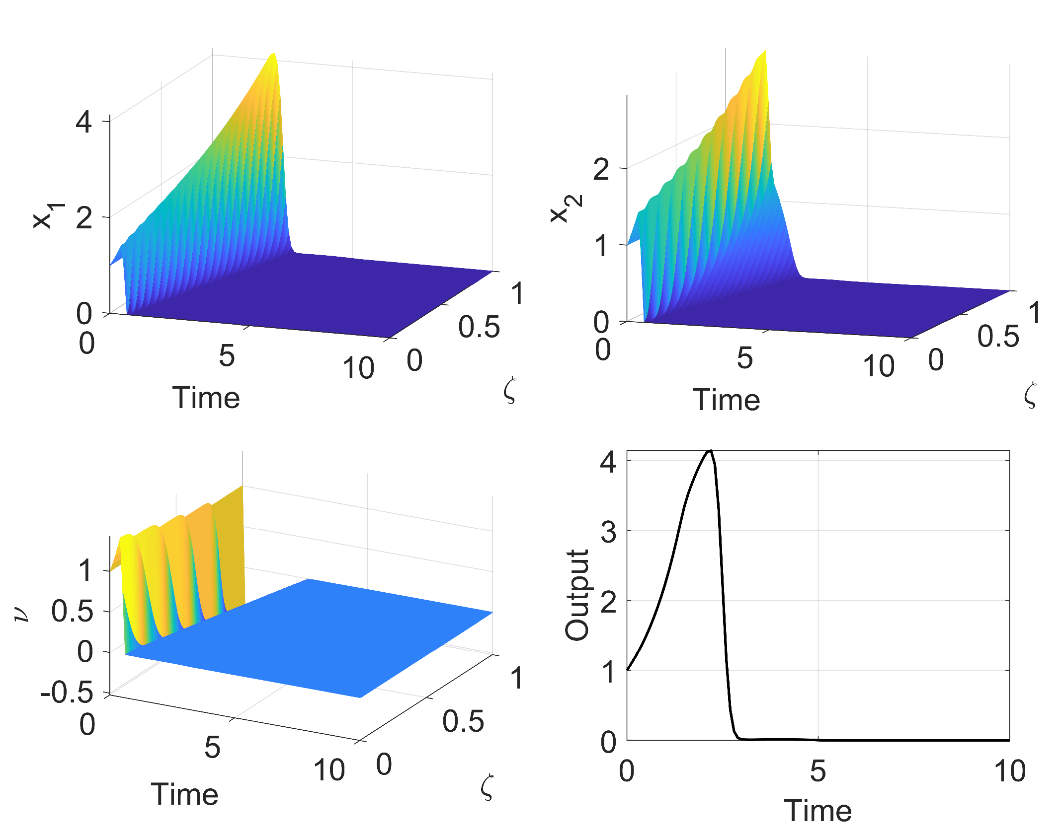
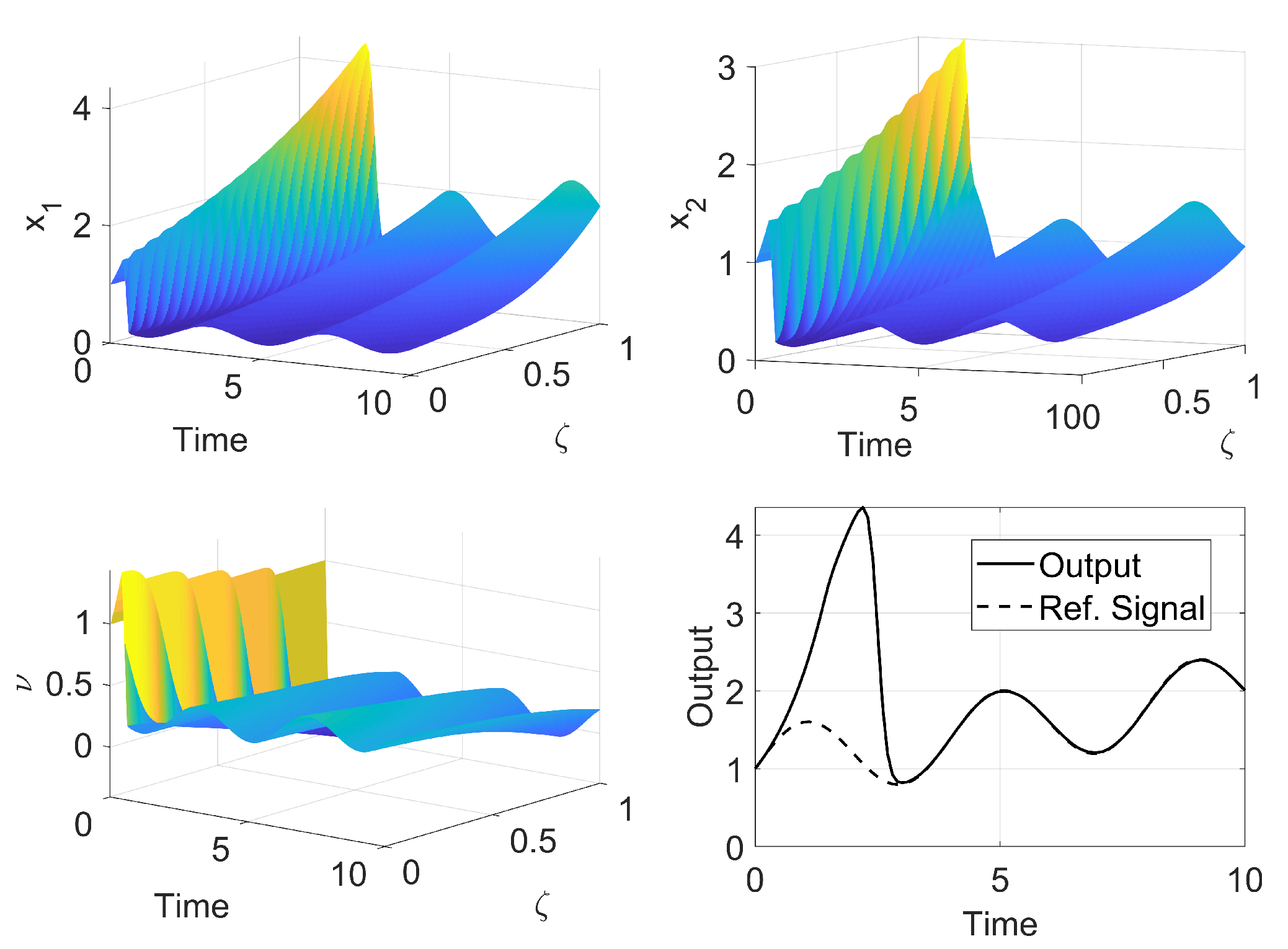
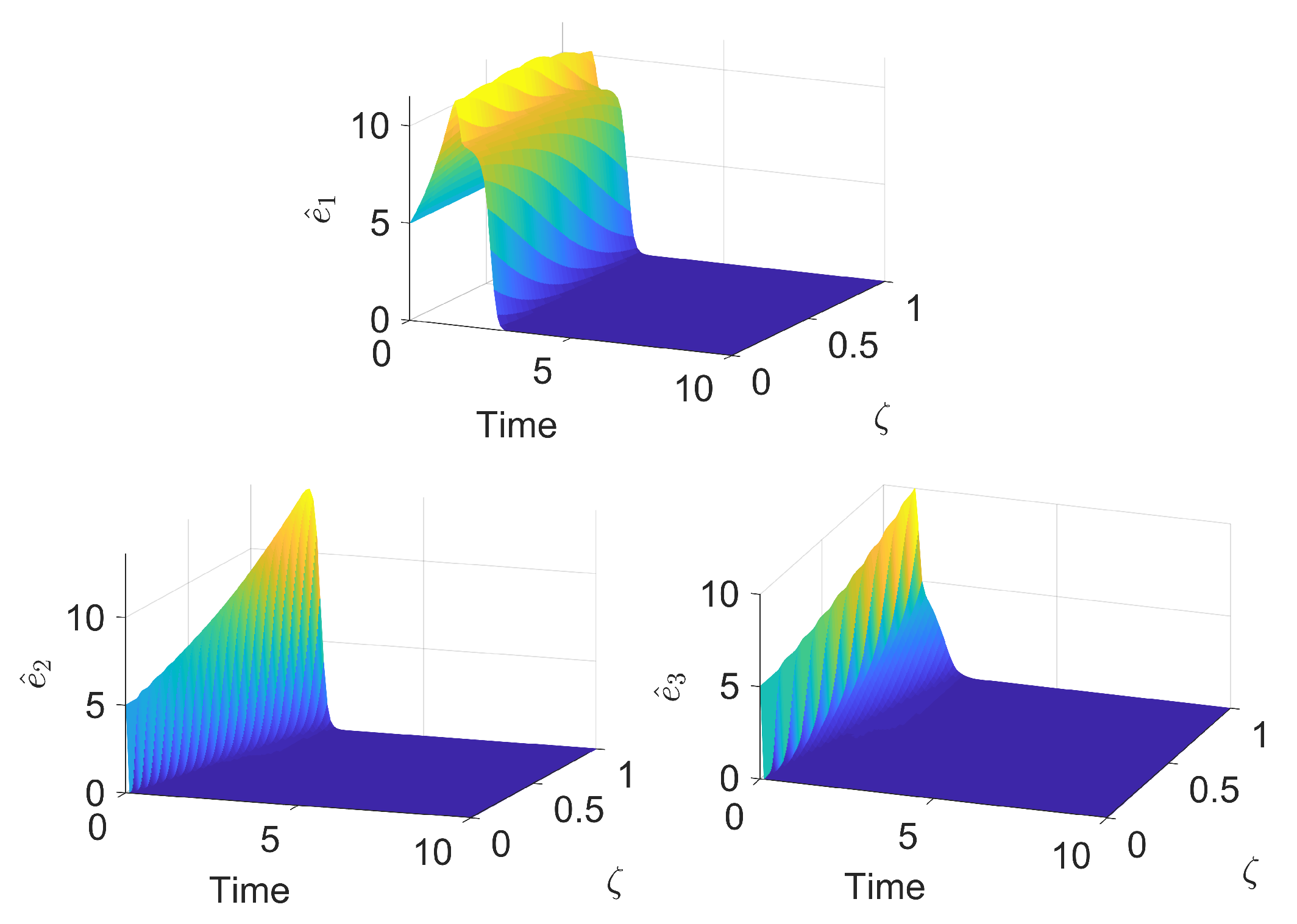
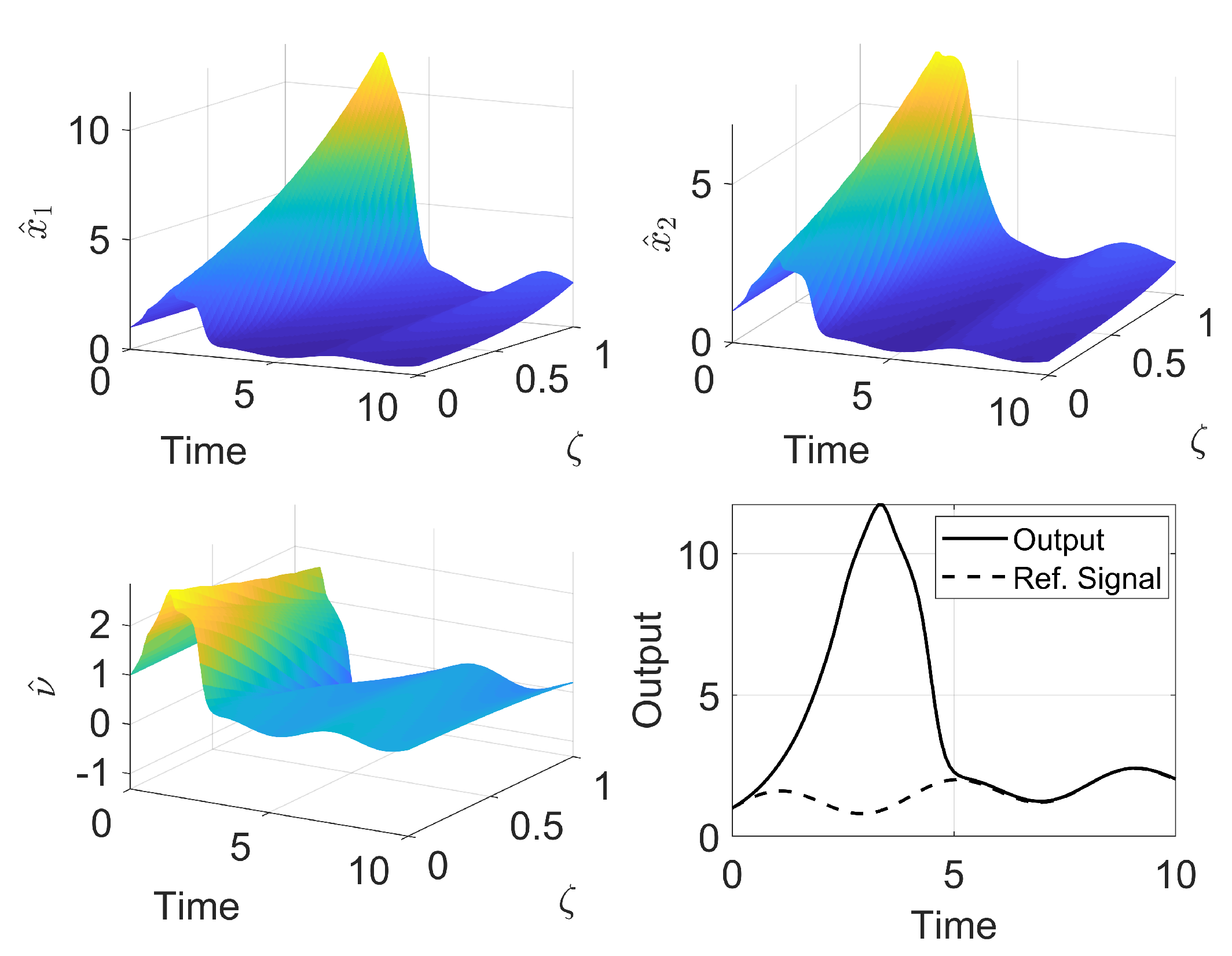
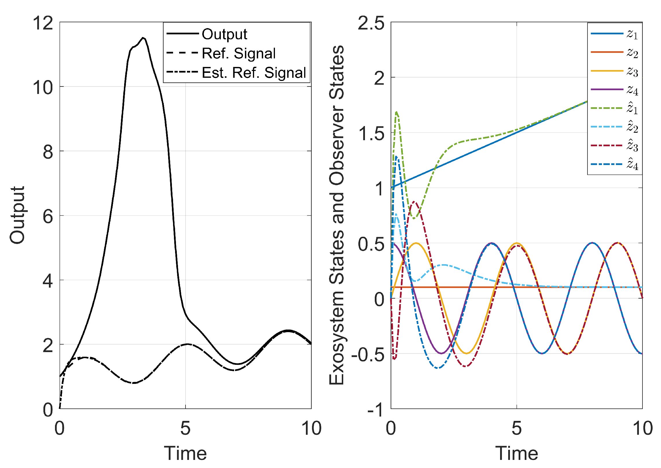
In this manuscript, the regulator design for the Saint–Venant–Exner model was developed so it would achieve proper closed-loop stability and output tracking of a reference signal in both continuous and discrete-time setting. The backstepping methodology was used in the continuous-time setting to map the closed-loop system to a stable target system, thus guaranteeing the system stability. Furthermore, the same method was used to design the observer, allowing for the reconstruction of the system states by using just the output. Considering a reference signal generated by an exosystem, the output tracking problem was solved. Next, with the stabilization and proper tracking achieved in the continuous-time setting, the discrete regulator was explored. The closed-loop stability, observer design and the regulator equations were shown to be directly related to their construction in the continuous-time, thus ensuring the proper performance of the regulator, as it was possible to observe in the simulations.
For future work, the constrained optimal stabilization and tracking problem could be considered, as the regulator designed here did not take into account any physical limitations, neither in the states nor the input.


