Real-Time Decision-Support System for High-Mix Low-Volume Production Scheduling in Industry 4.0

Abstract

Numerous organizations are striving to maximize the profit of their businesses by the effective implementation of competitive advantages including cost reduction, quick delivery, and unique high-quality products. Effective production-scheduling techniques are methods that many firms use to attain these competitive advantages. Implementing scheduling techniques in high-mix low-volume (HMLV) manufacturing industries, especially in Industry 4.0 environments, remains a challenge, as the properties of both parts and processes are dynamically changing. As a reaction to these challenges in HMLV Industry 4.0 manufacturing, a newly advanced and effective real-time production-scheduling decision-support system model was developed. The developed model was implemented with the use of robotic process automation (RPA), and it comprises a hybrid of different advanced scheduling techniques obtained as the result of analytical-hierarchy-process (AHP) analysis. The aim of this research was to develop a method to minimize the total production process time (total make span) by considering the results of risk analysis of HMLV manufacturing in Industry 4.0 environments. The new method is the combination of multi-broker (MB) optimization and a genetics algorithm (GA) that uses general key process indicators (KPIs) that are easy to measure in any kind of production. The new MB–GA method is compatible with industry 4.0 environments, so it is easy to implement. Furthermore, MB–GA deals with potential risk during production, so it can provide more accurate results. On the basis of survey results, 16% of the asked companies could easily use the new scheduling method, and 43.2% of the companies could use it after a little modification of production.

1. Introduction

Market diversification and ever-changing, uncertain demands urge many enterprises to speedily respond to expected customer satisfaction. High-mix low-volume (HMLV) production is a category of processes that allow for a high variety of products to be produced in relatively small amounts. The high variety of products in question causes a number of complications in the implementation of several production-scheduling techniques. Many products are highly customized according to various demands that are nonrepetitive and require completely different processing sequences. The cycle time for each production process of each product is irregular, and the predictability of the process is problematic and complex [1]. The HMLV production process is currently a global trend that requires a high degree of customization and high frequency of machine changeover [2,3,4]. Many manufacturing industries need to use different varieties of production-scheduling methods in order to increase productivity and reduce production costs [5,6]. Production scheduling in several manufacturing industries has been extensively applied over the past few years, and continues to be increasingly demanded in this era of cyber–physical systems and digitized-manufacturing environments. The invention of new and advanced production-scheduling methods is becoming imperative in today’s digitized manufacturing [5,7]. Scheduling means the allocation of resources and the sequence of jobs for the production of goods and services. The production schedule determines when each job begins and ends on each machine. Scheduling is an act of determining priorities or organizing activities to meet certain requirements, constraints, or objectives [8,9]. Predictive–reactive scheduling approaches generate a predictive schedule offline (before production begins) and correct the given schedule online (during production) [10]. The smart-scheduling layer primarily works with advanced models and algorithms to calculate with recorded data by sensors. Data-driven techniques and advanced decision architectures can be used for smart scheduling, for example, to achieve real-time, reliable scheduling with the use of a smart distribution model to generate a hierarchical interactive architecture [11]. Real-time decision-making is the provision of information in context that is integrated with the workflow in real time and that can be applied to any device, anywhere, any time, for making decisions. In the context of production scheduling, smart sensors are inevitable in real-time decision making.

Digital manufacturing is an integrated type of manufacturing controlled by a computer system that has proven to be a promising form of manufacturing in Industry 4.0. Digital manufacturing is more realistic when conventional manufacturing technologies are combined with digital techniques [12]. There are a number of key factors to consider when implementing digital manufacturing, and several areas where digital manufacturing works well [13]. Industry 4.0, or the Fourth Industrial Revolution, refers to closed and connected systems that blur the boundaries between real and virtual factories, represented by cyber–physical systems (CPSs). Big data are large databases that are constantly updated and cannot be analyzed by conventional methods [14,15]. A cyber–physical system (CPS) is a system of collaborating computational elements that controls physical entities. A CPS is a physical and engineered system whose operation is monitored, co-ordinated, controlled, and integrated by a computing and communication core. Industry 4.0 can be described as the interconnection of production systems with a cyber–physical system. An essential component of Industry 4.0 is the cyber–physical system that can be described as an embedded system that relies on sensors to record data and manipulate physical processes with the help of actuators operated in digital networks [16]. On the basis of a number of literature reviews, the most relevant core elements are connectedness, smart machines and products, decentralization, big data, and cybersecurity [17]. CPS is described by its three main characteristics: intelligence, connectedness, and responsiveness to changes [16]. Combinations of real and big data also offer new opportunities for process planning. The process model is developed by a machine-learning algorithm combined with a metaheuristic so that several sets of optimized process parameters can be derived.

1.1. Problem Description

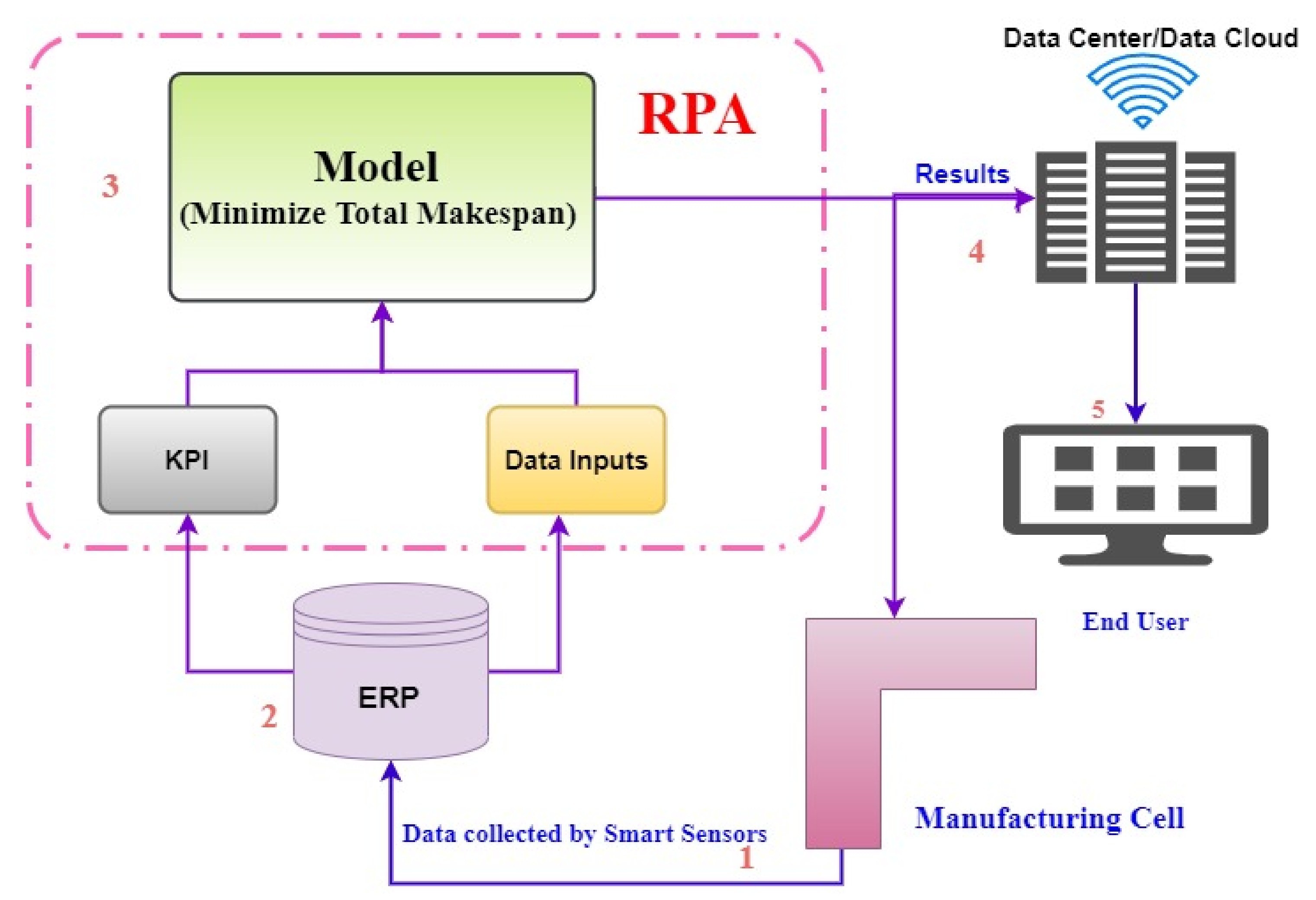
Figure 1 below illustrates the general concept of the problem to be solved. The assumption is that there is a manufacturing cell that includes more than five machines and more than 10 jobs, so a number of activities must be performed by the given machines. Production scheduling is the key problem, and the idea behind it is to automate the new production-scheduling model with the help of robotic processing automation. The developed model involves the extraction of information from the enterprise-resource-planning (ERP) system, where key process indicators (KPIs) and production inputs are key factors for the model. ERP information is collected by smart sensors that are installed on each machine and are able to read the attached workpiece information to be processed on a given machine in respective sequence. The newly developed model provides results that the robotic process automation (RPA) uses as a decision-making point to achieve the lowest cost and least tardiness.

1.1.1. Mathematical Model

Jobs $J=J_1,J_2,\dots ,J_n$ is a set of n independent jobs to be scheduled. Each job $J_i$ consists of a sequence $O_{i}1,O_{i}2,\dots ,O_i{n}_i$ of operations to be performed one after the other according to a given sequence. All jobs are available at time 0 for each machine. The letter $M=M_1,M_2,\dots M_m$ represents a set of m machines. Every machine performs only one operation at a time. All machines are available at time 0 [18]. HMLV production is generally classified into two categories: each machine can be processed by any of the M machines, and each operation can be performed only on a subset of M machines.

1.1.2. Further Assumptions

Assumption 1.Every operation is processed by only one machine at a time;

Assumption 2.Operation processing times are independent from one another;

Assumption 3.Pre-emption of operations is not allowed, i.e., any operation, once started, must be completed without interruption; and

Assumption 4.The required setup time to program to process an operation is included in the job-processing time.

On the basis of these assumptions, the mathematical model of production scheduling is as seen below:

• $N=$ total number of jobs;
• $M=$ total number of machines;
• $G_i=$ total number of alternative processing plans of job i;
• $O_{i}jl=$j-th operation in l-th alternative process plan of job i;
• $P_{i}l=$ number of operations in l-th alternative process plan of job i;
• $k=$ alternative machines corresponding to $o_{i}jl$;
• $t_{i}jlk=$ earliest completion time of operation $O_{i}jl$ on machine k;
• $C_{i}jlk=$ earliest completion time of operation $O_{i}jl$ on machine k;
• $C_i=$ completion of job i;
• $T_i=$ tardiness of job i; and
• $L_i=$ lateness of job i.

The aim of this research paper was to develop a new advanced and effective real-time production-scheduling decision-support system model that could deal with production-risk analysis in real time. The developed model was implemented by the use of robotic process automation (RPA), and it is the hybrid of different advanced scheduling techniques obtained as the result of analytical-hierarchy-process (AHP) analysis. The aim of this research was to develop a method of minimizing total production-process time (total make span), and to perform risk analysis of HMLV manufacturing in an Industry 4.0 environment.

The subject of this paper is a critical evaluation of the literature review on real-time decision-support methods, production-scheduling methods, and the identification of key performance indicators—the requirements of Industry 4.0. The paper analyzes the gap and devises improved methods or models that are suitable for HMLV manufacturing industries.

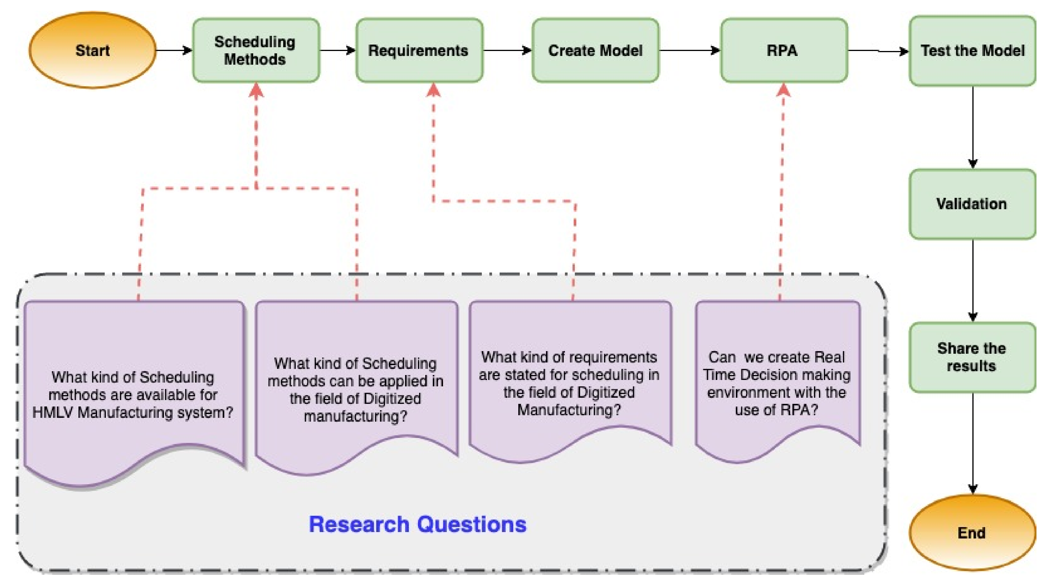
Figure 2 below shows the positions of the research questions for each step to be performed.

1.2. Production-Scheduling Techniques

A heuristic method was proposed for scheduling multiple projects subject to cash constraints [19]. The heuristic was used to determine cash availability during a given period by identifying all possible activity schedules.

1.2.1. Genetic Algorithms

This is a metaheuristic inspired by the process of natural selection, where the process begins with a set of individuals called a population, and each individual is a solution to the given problem. An individual may be a set of variables called genes. Genes are combined to form a chromosome that can be interpreted as a “solution” in a scientific context in engineering manufacturing. The following step, called the fitness of the function, is observed to reveal how good it is through the fitness score of the values, and each score is based on probability [20,21,22,23,24]. Along with appointing individual members fit for the job to be performed, another perpetuation of the next generation is also selected. The best selected individuals are then crossed, that is, followed by mutations, until the desired solution is reached. Complex problems can be solved with the use of genetic algorithms that are capable of finding an optimal solution [25,26]. GA is a natural process of evolution in biological sciences, and it has the power of solving heuristics-related problems [23,27]. The authors in [28] used a modified version of genetic algorithms to solve flexible job-shop scheduling problems (JSPs). Genetic algorithms are a subset of stochastic-search algorithms that can serve as a very effective selection method for discovering optimal solutions to a wide range of problems. The purpose of applying a modified genetic algorithm was to minimize the makespan of the JSP. When applying a GA, the following parameters must be set: encoding method, chromosome length, population size, mating method, crossover method and rate, mutation method and rate, fitness method, selection mechanism, and termination condition [27,29,30].

GAs are used to generate high-quality solutions for optimization and search problems by relying on bioinspired operators such as mutation, crossing, and selection. To perform a GA, there must be a specific sequence of tasks and start times (genes) that represent a genome of our population.

1.2.2. Hybrid Optimization Scheduling Method

This method aims at combining the above two or more approaches to create a more effective and efficient production-scheduling method. The hybrid approach combines the Mixed Integer Programming (MIP) model, the simulation model, and the genetic algorithm as follows. First, the MIP model is used to obtain an optimal schedule for production and transportation processes in terms of supply-chain costs, considering the system in a purely deterministic way. Subsequently, the simulation model is used to evaluate the performance of this obtained schedule in terms of the number of resulting delayed orders, where stochastic behavior is based on probability distributions [26,27,29,30,31,32,33]. It belongs to the group of solutions to a given problem within a short period of time.

1.3. Multibroker–Genetic-Algorithm (MB–GA) Scheduling Method

The volume of available data is exponentially increasing in the case of industrial processes. Furthermore, additional Internet of Things (IoT) tools are being invented and utilized every day [34]. Considering these facts, manufacturing processes are fundamentally changing. This results in the more effective use of production-scheduling techniques than traditional ones. If manufacturing data are available and accessible, decision makers can take the risks into consideration during the planning phase of production, as well as interference in the operations of the system when deviation is detected.

The newly developed multibroker genetic-algorithm (MB–GA) scheduling method uses general KPIs and parameters, and this is why it is not industry-specific. It is suitable for scheduling production programs in the HMLV industry. The values of these parameters are easy to measure, and KPI values are easy to calculate.

The developed method is compatible with different maturity levels of Industry 4.0. If the company has a high maturity level in Industry 4.0, the process of Hybrid scheduling model by RPA can easily be implemented where data are gathered by sensors and optimization is automatically run by RPA. If the company has a low level of maturity, it can use just the optimization part, where input is manually gathered for optimization.

Compared to other methods, such as linear programming, heuristics, and genetic algorithms, this MB–GA scheduling strategy is a multilayer-filter approach that considers the workload and job-cost ratios of the system. It is flexible and easy to operate in Industry 4.0. This method supports multiobjective function and parallelism, it is easy to modify, and adaptable to various problems and time-consuming results.

The new MB–GA method is compared to other scheduling methods by RPA with respect to attributes of Industry 4.0, and the new method has a massive advantage in the field of flexibility.

2. Background

The attributes and techniques of Industry 4.0 are presented in this section. These attributes and techniques were taken into consideration as requirements during the development of the new scheduling method.

2.1. Industry 4.0

Over time, extensive literature was developed on real-time decision-support systems for planning and scheduling operations in Industry 4.0. This paper begins with a brief review of the literature on production-scheduling methods and techniques; however, the question arises as to whether these methods can be sufficiently synchronized with Industry 4.0 environments. The Internet of Things, big data, cloud computing, simulation, augmented reality, robotics, additive manufacturing, cybersecurity, and the integration of horizontal and vertical systems, are keywords of Industry 4.0. The Industry 4.0 concept is associated with the technical perspectives of the integration of cyber–physical systems (CPSs) into manufacturing operations, and the integration of Internet of Things (IoT) technologies into industrial processes represented by smart factories, smart products, and extended value networks. They are vertical, horizontal, and end-to-end integrations [35,36,37].

The novel production process, identified as digital manufacturing in new factories, combines Industry 4.0 technologies, including 3D printing, the Internet of Things, big data, simulation tools, and three-dimensional visualization [38]. The authors in [39,40] highlighted the importance of real-time scheduling in HMLV manufacturing, emphasized the use of group sequences as a decision-support system, and further explained that real-time decisions can be categorized into three types: decisions to start processing an operation, decisions to interrupt the processing of an operation and at the end of a processing-unit breakdown, and decisions to resume the processing of the interrupted operation assigned to the resources. The group sequence of the permutable operations was proposed to be used as a subset of the available scheduling methods.

The authors in [41] proposed overtime scheduling, an application in finite-capacity real-time scheduling that determines which work centers are needed, and when and how much overtime is required to meet the requested due time within the overtime cost. A finite-capacity real-time scheduling and planning system was used. In [18], the authors investigated the integration of smart manufacturing and Industry 4.0 production environments with physical and decisional aspects of manufacturing processes in autonomous and decentralized systems. Smart scheduling was introduced to achieve a flexible and efficient production schedule on the fly in a 4.0 environment equipped with cloud computing, Internet of Things (IoT), big data, and radio-frequency identification (RFID) technologies that are intertwined in a way in which work is done, and business logistics processes are performed and reported in the ERP system in real time.

According to the author of [42], there are different types of decision-support systems. Data-, model-, knowledge-, document-, and communication-driven systems are the most common decision-support systems (DSSs); in addition, intelligence- and data-driven DSSs are highly preferred. Big-data analytics combined with learning agents and deep-learning toolkits, and trained with artificial neural networks, simulations, and forecast toolkits can provide substantial information and data to a DSS. A multiagent-based system is a complex autonomous and intelligent system that is popularly applied in production scheduling, and its applicability is determined as agents that represent subsystems. Each agent determines its own course of actions and other agents may influence an agent’s decision by means of co-ordination or collaborations. Agents representing subsystems can solve problems within their domains with their own of control and execution. Each agent executes its own work without being dependent on another agent.

The author of [43] studied the development of a real-time monitoring system as a decision-support system for flood-hazard mitigation. In this study, photography, communication, geometry-information display, and network technology were used to provide real-time monitoring images at critical gauge stations, and it suggested that users should use mobile phones to receive or report real-time flood-related information at any place and time.

2.2. Robotic Process Automation (RPA)

RPA is an umbrella term for tools that operate similarly to a human by being on the user interface of another computer system [44]. The application of this technology allows for computer software to partially or fully automate human activities that are manual, repetitive, and rule-based. It normally applies the “if/then/else” rule [44]. RPA allows for a company to map a definable, repeatable, and rule-based business process, and assign a software “robot” to manage the execution of that process. It is assumed that 22% of IT jobs can be replaced by robotic process automation in coming years, and all non-value-added steps were shown to significantly exceed 40% [45]. RPA increases efficiency and effectiveness by reducing the workforce through the so-called “digital workforce” [45]. According to [46], RPA has a technical infrastructure that includes

• interactive clients (developer or controller);
• runtime resource PCs (1–10 robots per pc);
• application servers (service, I per 100 robots); and
• database (1 per environment).

For [47], an RPA system includes IoT devices and a server as part of the subnetwork for secure communication relating to high-mix low-volume production processes. Robotics is where machines mimic human actions; the process is a sequence of steps to perform a task, and automation performs any meaningful task without human intervention [47,48,49]. The authors of [50] explained that RPA is the wave of innovation that will change outsourcing strategies; it was launched as an experiment at Telefonica O2 in 2010 and was designed for high-volume low-complexity processes. This company implemented Blue Prism as an RPA. RPA does not rely on/involve any inventions of software or technology for automation. The same RPA tool can be used to automate various projects that use different technologies and do not require human intervention. More than 12 companies participate in RPA, but the top three companies are Automate Anywhere, UiPath, and Blue Prism [51]. Automate Anywhere is recommended to be used for forward office (FOR) and backward office (BOR) robotics, UiPath performs well in FOR, and Blue Prism is efficient in BOR robotics. Robotics: machines that mimic human actions are called robots.

Process: a sequence of steps that lead to a meaningful activity, for example, the process of making apple juice.

Automation:Any process that is done by a robot without human intervention. In summary, imitating human actions to perform a sequence of steps that lead to a meaningful activity without any human intervention is known as robotic process automation.

RPA Tool Features

• Web automation: this feature allows companies to automate web interactions by identifying web elements and accurately manipulating them.
• GUI automation: The process of simulating mouse and keyboard actions on Windows, and it controls screen scraping. This is the process of extracting text from websites and win32 apps.
• Microsoft automation: automating Microsoft Office applications may be the most commonly used feature of RPA tools.
• Citrix automation: surface/Citrix automation is used because components of virtual machines cannot be accessed.

A study conducted by [44] to show the position of RPA in system, seen by many organizations as a way to quickly achieve a high return on investment [44]. Debates still continue as to whether it should be used tactically or strategically [52,53].

2.3. Process Monitoring

The monitoring process for an HMLV production schedule must consist of three basic interconnected components: (a) database; (b) scheduling engine; and (c) user interface (UI).

2.4. Model Requirements

• Due/finishing date of the job;
• processing time of each the job;
• maximal completion time of the job;
• job weight;
• preparation time for start-up;
• number of jobs to be processed;
• steps to be taken during the job;
• starting time of the job on a given machine;
• number of machines
• expected needed time to process the job;
• permutation job setting;
• number of orders;
• priority of orders;
• task priority (task value);
• variance of time needed to process the job on a given machine;
• waiting time; and
• worker walking time.

2.5. Manufacturing-Environment Requirements

2.5.1. Forecast of Customer Demand

Demand is a fundamental key aspect in high-mix low-volume production scheduling. It is a triggering parameter to start production, and it justifies the existence of a company in a competitive world. Knowing demand in real time helps to apply the just-in-time philosophy. Despite the dynamic nature of demand in HMLV manufacturing systems, demand forecasting is still very important to some extent. Forecasting means making a present approximation about a future occurring event, and demand means requirements for products and/or services to be sold or supplied to the customer. The developed model in question must be able to integrate with the customer database, which can be achieved through the connection of the model to the ERP system. The developed model is operated by a robotic-process-automation system.

2.5.2. Available Resources in Real Time (Labor, Machines)

The availability of labor and machines in real time is as crucial as having an engine in a car. Machines perform the jobs, and human resources operate the machines. Without having smart machines and smart workers, it is impossible to implement smart scheduling in Industry 4.0 environments. For the availability of machines, continual maintenance is required. Lean philosophy and a total quality-management system must be applied in order to utilize machines and labor to maximal efficiency.

2.5.3. Bill of Materials (BOM)

The expected duration of scheduling throughout the production process is highly dependent on many factors, including the availability of raw material. If raw materials are well-organized and appropriately described, it facilitates scheduling to be realistic during optimization. Before costs of manufacturing are determined and quoted on the basis of customer orders, it is possible to create a BOM, which is one of the subsets and key data in material-requirement planning (MRP). Other key data can be the availability of computerized production and inventory systems, and a complete list of components that constitutes a prototype, an assembled, or usable product. In most cases, the bill of materials includes the following elements: quantity, item ID no, description, and cost, and total project cost [54].

Takt time considers the average production working time of the manufacturing process [55]. It is the pace in which a product must be produced in order to satisfy customer demands, or the desired time required to produce a unit of production output. From customers’ point of view, takt time means feasible operating time tailored to their needs. From an operational point of view, takt time is an initial design variable that dictates the architecture of the entire manufacturing operation. Therefore, takt time is the piece of data that shows how fast to produce according to the desired product demand. Takt time is used for efficient workforce and capacity planning, and for controlling processes by finding bottlenecks and constraints during production [56,57].

$$\mathrm{Takt}\mathrm{time}=\frac{\mathrm{Net}\mathrm{time}\mathrm{available}}{\mathrm{Total}\mathrm{customer}\mathrm{demand}}$$

(1)

Takt time cannot be measured by a stopwatch, but it can be calculated by the formula above.

2.5.4. Available Event Logs

Event logs are crucial as a starting point for any process mining. Event logs (data management), product data, process, resources, model, and scenario all need to be linked to the ERP system that works together with HMI and SCADA, and provides data import and export facilities with path, feedings, equipment, and handlers. The process-planning level to control level has to be combined from the performance system of manufacturing [58,59,60].

2.5.5. Internet of Things (Connectedness)

IoT refers to the network of interconnected every-day items that are often equipped with ubiquitous intelligence [61,62]. The Internet of Things (IoT) is the inter-related system of physical computing devices that can be accessed via the Internet [63]. The Internet of Things can refer to any object, machine, or person that is capable of transmitting and collecting data without external support as Figure 3 presented. There are four components of the Internet of Things: sensors, connectivity, people, and processes. The IoT refers to objects with sensing or processing capabilities, each assigned a unique IP address that communicates data over the Internet without the need for human interaction. In a broader sense, the IoT includes artificial-intelligence, cloud-computing, next-gen-cybersecurity, big-data, twin-simulation, augmented- and virtual-reality, blockchain, and advanced-analytics technologies [63,64,65,66,67,68,69]. Technologies that support the Internet of Things include 802.11 Wi-Fi, 802.16 Wi-Max, 802.15.4-LR WPAN, 2G/3G/4G mobile communication, 802.15.1 Bluetooth, and LoRaWAN RI.O (LoRA) [70].

2.5.6. Sensors and Actuators

Human sensors, user inputs, documents, environment sensors, localization, motion, and actuators [61,62] are data inputs for many smart devices.

2.5.7. Monitored Production

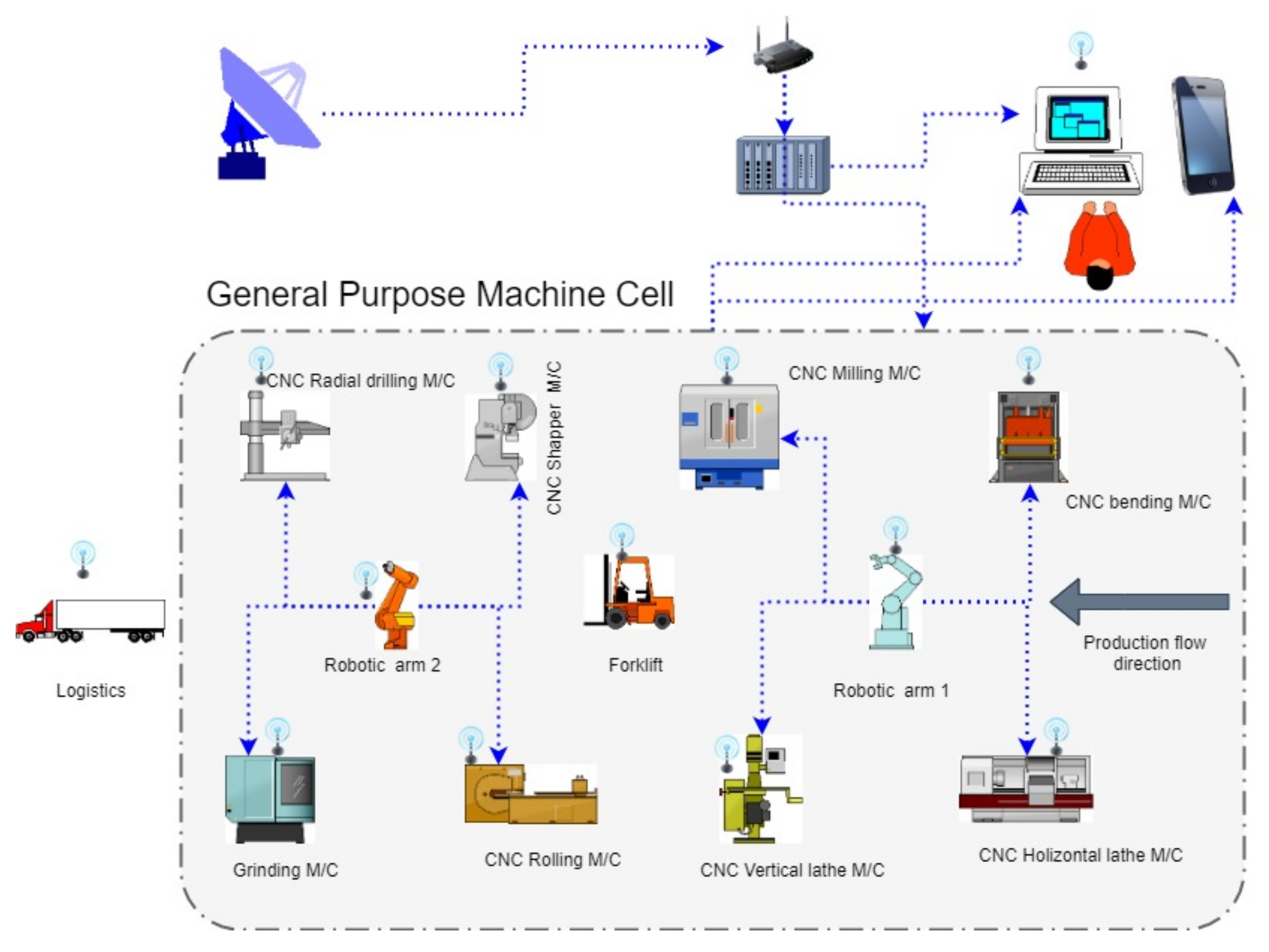
Monitoring production is one of the key factors in Industry 4.0 environments. Figure 4 shows a monitored general-purpose machine cell, where each machine in the cell is connected to Wi-Fi that sends signals to every machine depending on the task at hand.

2.5.8. Product Cycle Time

Most companies that involve customers at the stage of product design and development may experience shorter cycle times and realize higher profits as compared to firms whose customers are not involved. Cycle time is the time interval between finished goods, and it is the actual time that it takes for an employee to complete one cycle of their process. Cycle time can be measured by a stopwatch. Measured cycle time helps to determine the reliability of the system, and it is one of the determinants in the digitized environment among production-scheduling methods. If data were previously collected in the event log, cycle-time analysis can be performed by descriptive statistics that are then used to monitor deviations in the actual production stage [71].

2.5.9. Control System

The designed production-scheduling model needs to show the control of delivery time, costs, and quality of the product being produced. If the model can show the scheduled production in a Gantt chart, then that production can be visualized and controlled. During the actual execution of production processes, a control system is needed to ensure that scheduled production is maintained as planned. Cycle-time variance is under control. After calculating statistical analysis of the cycle time (mean, mode, and median), it is possible to monitor and control the variances. The task is to ensure that total optimized tardiness (minimized) is maintained throughout production. The most important factor in tracking/monitoring and performing cycle-time analysis is the elimination of work stoppages [72].

2.5.10. Inventory Level in Real Time

The authors in [73] developed a probabilistic form of standard material-requirement planning (MRP) in production planning for product remanufacturing. It considers variables of yield ratios of good, bad, and repairable components collected from incoming units, as well as those of probabilistic processing time and yield at each stage of the remanufacturing process. MRP is a general approach to production planning in a traditional manufacturing environment. Altendorfer (2019) investigated the interaction of different planning parameters, loT size, safety stock, and planned lead times for different items in his study titled “the effect of limited capacity on optimal planning parameters” in a multi-item production system, where information about setup times and advance demand had been provided.

2.5.11. Available ERP System

ERP is a packaged software system that enables the consolidation of operations, business operations, and functions through common data-processing and communications protocols [6]. As the number of jobs increases, the complexity of the scheduling problem is manifested through common data-processing and communication protocols. The American Production and Inventory Control Society [74] defines ERP as a method of effectively planning and controlling all resources that record data about manufacturing, delivery, and customer orders during production, distribution, and service. ERP links all areas of a company, including operations and logistics, sales and marketing, human resources, and finances. ERP traces its roots to material-requirement planning (MRP) and manufacturing-resource planning (MRPII). Consulting and other costs should also be considered when determining ERP software and hardware costs. ERP enhances a company’s competitive and strategic advantages. Integrating ERP in high-mix low-volume production scheduling results in the reduction of wasted resources in the form of materials, energy, inventory defects, wasted capacity, labor control, and work-in-progress control. The reduction of waiting, cycle, and setup times, and delays can also be realized with ERP, and it can efficiently co-ordinate the work of all departments within an organization [6,74,75,76,77,78,79].

3. Materials and Methods

The steps of the research were the following:

• Analysis of high-mix low-volume production-scheduling techniques, manufacturing-system environmental requirements (Industry 4.0 environments), and model requirements.
  First step: intensive literature review of scheduling techniques, manufacturing-system environments, and model-system requirements was implemented.
  Second step: creating a list of scheduling techniques, manufacturing system requirements, and model demand.
  Third step: creating the weighting-score list of the manufacturing list on the basis of their importance by their importance using the multicriteria decision-making technique.
  Fourth step: applying AHP to find the most suitable scheduling techniques on the basis of scores of the manufacturing-system and model requirements.
  Fifth step: Data on risk-analysis techniques used in SMEs and start-ups were gathered from five countries, namely, Croatia, Hungary, Poland, Slovenia, and Slovakia. The aim of the survey was to get a general view of the most common types of risk-analysis methods used by SMEs and start-ups to determine if the developed risk-analysis method was easy to implement or not. During the three-month-long data-collection period from December 2019 to March 2020, 199 responses were collected. However, 43 responses from large companies did not fit the scope of the project (the focus was on SMEs and start-ups); therefore, these responders had to be excluded from analysis. After data cleansing, there were 156 valid responses.
• The concept of a real-time decision technique, combined with time- and cost-based failure-mode and effect analysis controlled by RPA, was created.
• Taking properties of Industry 4.0 into consideration, the authors developed an MB–GA method for production scheduling. The developed model was compared with other scheduling methods existing in the literature in order to examine the new model’s performance and its advantages. For comparison, the AHP method was applied.

3.1. Hybrid Scheduling MB–GA Process Automated by RPA

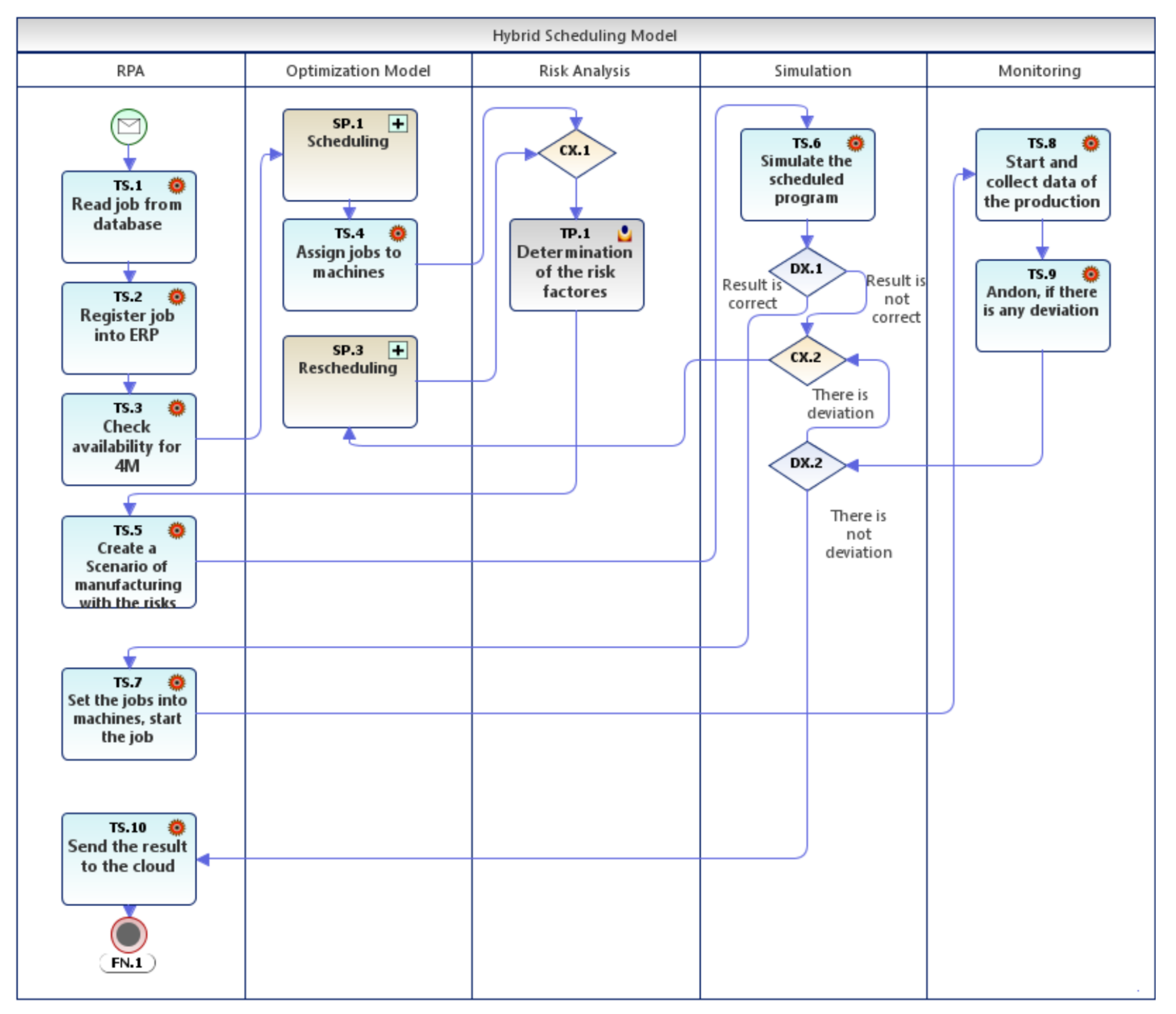
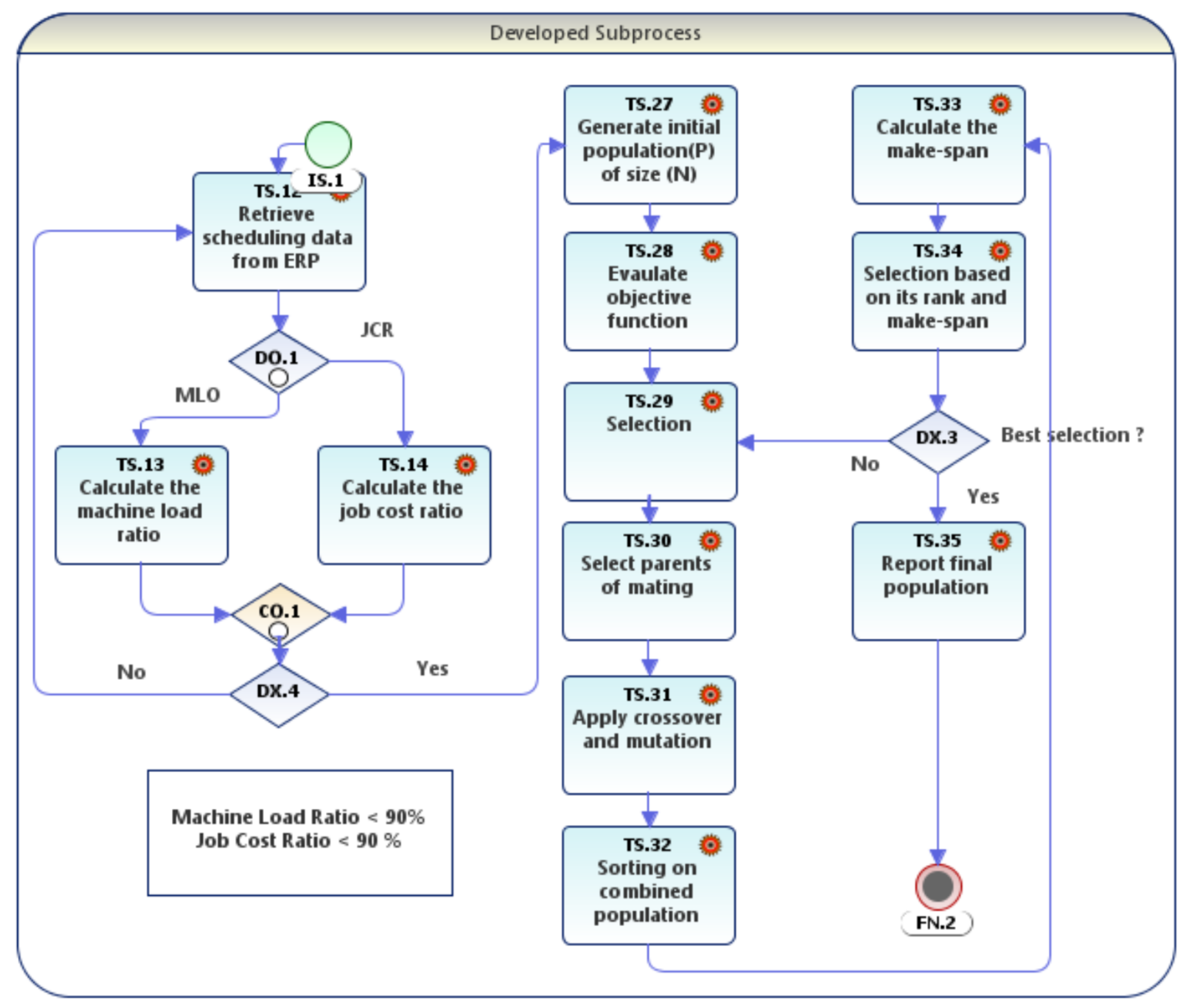
Figure 5 below presents the developed concept. The concept consisted of four main parts: (1) the heart of the system was MB–GA optimization as illustrated in Figure 6; (2) risk analysis, (3) when the optimal production program was simulated to see its possible result, and (4) when the production process was monitored. Every part could be performed by RPA. The input data arrived from the ERP system, and the RPA checked the resources. If there were enough materials, available machines, and operators, and all information was available, the optimizing engine started to find the best solution.

3.2. New Hybrid (MB–GA) Optimization Method

The new hybrid scheduling approach contains the multibroker (MB) and genetic-algorithm (GA) approaches to form the MB–GA production-scheduling approach. The scheduling protocol was structured in such a way that the multibroker is aconfigured first, and the agents’ performance is used as the deciding factor for more processing in the genetic algorithm. This work considered only two variables that are eligible for decision making that involved the collection of available resources in real time. The factors used in this optimization process can be seen below.

Machine–workload ratio agent: the machine workload ratio is the measure of how busy machines are at the respective time of scheduling, and it can be calculated as follows.

$$MWLR=\sum \frac{SetupTim{e}_{i}j+Quantit{y}_{i}j*RunTim{e}_{i}j}{MachineCapacity*QuantityofMachines},$$

(2)

where MWLR is the machine-workload ratio.

From the above equation, if workload load ratio was higher than the given threshold factor, let us assume that it was 90%, it implied that the machine was busy by that percentage and omitted during real-time scheduling.

Job-cost ratio: the job-cost-ratio (JCR ) factor was obtained by the summation of all costs in a respective machine, as shown below.

$$JCR=\sum \frac{MaterialMovementCos{t}_{i}j+SetupCos{t}_{i}j+RunCos{t}_{i}j}{TotalCost}$$

(3)

The MB–GA scheduling algorithm began by extracting data from the ERP in .csv form. The extracted data were compared on the basis of predefined criteria that may be specified by the production manager as a cut-off point or a selection threshold for the optimization exercise. The deciding factor in this article was the workload ratio of the machine and the cost ratio of the job. When both variables were less than 90%, they satisfied conditions for the next stage of generating the initial population for the optimization process. When conditions were not satisfied, the procedure must be repeated. Generation of populations was accompanied by the creation of the objective function, the general selection process, and the selection of parents for mating. The application of the crossover and mutation rate was another step, followed by the classification of the combined population, makespan calculation based on its rank, and, after obtaining the best selection, drawing up the report as the final population.

Input data: The data inputs required in the MB–GA scheduling methods were: required time to transfer each job to the machine, setup time for each job on each machine, run time for each job on each machine, steps/operations needed for each job in each machine, cost of transferring every job from every machine, job-setup cost for each job on each machine, the processing time cost of each job in each machine, the number of machines required for each job in a plant, and the capacity of each machine (quantity/time).

3.3. Risk Analysis

In order to find the best production program, possible risk has to be considered in the planning phase. A multiobjective approach was developed by [80] that dealt with risks, so it is important to consider different risks and uncertainty during the process of optimization. Traditional failure-mode and -effect analysis (FMEA) is not compatible with this approach due to its subjectivity, so in the presentation of the new method, modified time- and cost-oriented failure-mode and -effect analysis was used.

Risk calculation of failures in time- and cost-oriented FMEA is determined on the basis of measurements. This method was invented by [81]. In this way, the subjectivity of the traditional method is reduced. The formula of time- and cost-oriented FMEA (tcFMEA) includes the probability factor of the situation where the total lead time given by Monte Carlo simulation in case of failures in the production exceeds planned total lead time. An essential part of tcFMEA is expected monetary value (EMV), which is used in the field of risk management. The goal of this tool is to quantify risks by calculating average outcomes for future failures that may or may not occur [82]. The impact value of EMV is the cost of failure and the cost of corrective activities in tcFMEA. The given parameters are the cost of the fixing process that is essential to eliminate a fault if it appears, the probability of failure occurrence, and the planned total lead time compared to the total lead time when the failure occurs. TcFMEA examines and compares different types of failures by the following formula. The calculation method can be seen below.

$$tcRPN=[(P_i*C_{ai}+P_e*C_{ae})+C_f]*F*T_p$$

(4)

• $P_i$ = probability of detecting fault before delivery;
• $P_e$ = probability of not detecting fault before delivery;
• $C_{a_i}$ = cost of corrective activities inside the company;
• $C_{a_e}$ = cost of corrective activities outside the company;
• $C_f$ = cost of failure;
• F = frequency of failure; and
• $T_p$ = 1+ symmetric-mean-absolute-percentage-error (SMAPE ) deviation between planned total lead time and estimated total lead time with failure, calculated by Monte Carlo simulation.

The most common and efficient way of analyzing manufacturing processes and complex production is to use a discrete-event simulation model [83]. As a numeric value is to be predicted in the know of various features, the prediction of a manufacturing lead time is a regression problem. To describe the prediction error, SMAPE is used.

$$SMAPE=\frac{1}{N}\sum \frac{|F_i-A_i|}{\left(\right|F_i|+|A_i\left|\right)/2},$$

(5)

where $F_i$ is the simulated and $A_i$ is the actual lead time of the $i-th$ job.

3.4. Simulation

The whole process was simulated after getting the optimal production program with the risks. The results of the process simulation were the estimated total process time (TPT), effective capacity, and first-time quality (FTQ). The minimal and maximal time values of the activities were calculated. Minimal time value was when an activity ran in the minimal time; maximal time value was when an activity ran for the longest time. Then, the coefficients of the function were calculated on the basis of the fuzzy-membership function. The formula below was used:

$$y=\frac{1}{1+e_i^a(b_i-x)}.$$

(6)

Relaying the function to x, we obtained the following formula.

$$x=b_i-\frac{ln\frac{1}{y}-1}{a_i},$$

(7)

where y is a random value between 0 and 1, $b_i$ is the intercept term, and $a_i$ is the coefficient for the single input value (x).

On the basis of the above equation, the possible cycle time of each activity was generated between the minimal and maximal time of the activity; consequently, value y was replaced by a random-number generator of between 0 and 1. Considering the logic of the process, the total process time of the process was simulated with 10,000 iterations. Standard deviation and the mean of the generated 10,000 process runs were calculated, and, with the inverse normal distribution function, the expected total process run time was calculated at a 95% confidence level. Effective capacity and first-time quality were calculated after the simulation. If TPT, capacity, and FTQ provided satisfactory levels, production could start. If not correct, rescheduling and resimulation were needed.

3.5. Monitoring

Tasks were delegated for each machine on the basis of optimization and simulation. Production started, and the key parameters’ production values were gathered by sensors in real time. The current status of the process was compared with the simulated value, and if there was any deviation, a revision was required. There was a possibility to take actions before a poor-quality product was produced or a delay was expected.

4. Results and Discussion

4.1. Risk Analysis during Scheduling

In real life, scheduling is basically an estimation of the duration of each activity sequence that will take place. The challenge is to determine the risk paths of operation activities without knowing the duration of activities. Many operation activities are presented as probability-distribution functions. Monte Carlo simulation and program evaluation review technique (PERT) are the most commonly used methods for the estimation of activity duration. Three-point estimation is the main method for collecting production-risk data that includes optimization, probable duration, and risk outcome. The main issue in production-scheduling risk analysis is the uncertainty of activity duration that is based on estimation error, variability, and discrete risk events. There are at least three risk categories, high (red), medium (yellow), and low (green). The limitation relies on the traditional approach that results from placing three-point estimation directly on the duration of activities. The main risk-driving forces in production scheduling are delays, disruptions, system risk, forecast of risk inventory, and capacity risk [84].

Different potential risks may occur during production. Many companies do not deal with risk and its evaluation. If companies ignore risks, they can lead to production loss [85] For accurate scheduling, potential risks must be considered. The use of traditional FMEA is not always appropriate, as it has a lot of shortcomings. They are

• decision-making problems [86];
• the human factor;
• FMEA is time-consuming;
• RPN values are not consistent; and
• RPN calculation is subjective [87].

The survey was evaluated where the current risk-analysis status of the companies was revealed in five countries. An essential part of the new MB–GA method is risk analysis. Survey results showed the companies’ readiness for the implementation of the new method.

On the basis of the survey, the following tables and figure provide information about

• type of risk-identification methods (

  Table 1. Methods of risk identification.

  Method Type	Number of Answers	Score in %
  Brainstorming meetings	75	40
  Multiple (or team-based) assessments	44	23
  Expert opinion (e.g., Delphi method)	38	20
  Historical data	31	16
  None of the above	1	1

  );
• risk categories (

  Table 2. Risk categories.

  Risk Category	Number of Answers	Score in %
  Financial risk	68	38
  Technical risk	64	34
  Commercial risk	48	27
  Political risk	1	1

  ); and
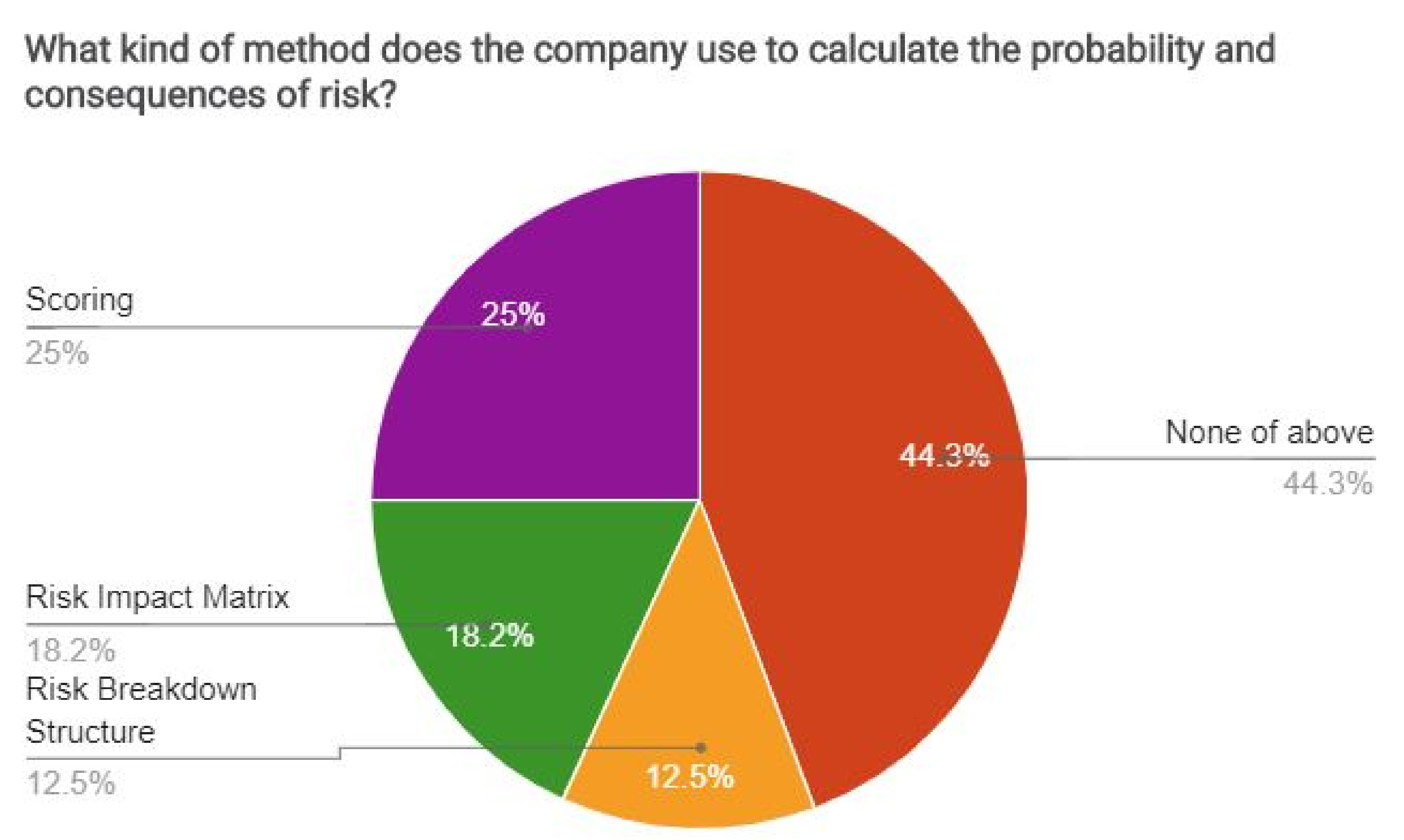
• the percentage of used risk-analysis methods (Figure 7).

Results can be seen in Table 1 and Table 2. The highest percentage of companies used brainstorming as a method or team-based assessments. Applying these approaches, traditional FMEA could be used to rank potential risk and root causes. Unfortunately, its reliability was low due to the subjectivity factor. Companies must have historical data to calculate time- and cost-oriented risk-priority number (tcRPN). Only 16% of companies had historical data for analysis.

In total, 25% of the companies used the scoring method to determine risk probability. If a company used scoring or a risk-impact matrix to calculate the probability, and possessed historical data, tcRPN calculation was easy to perform. The sum of the scoring risk-impact matrix was 43.2%, which means that 43.2% of the companies could calculate tcRPN. However, the problem was that only 16% had historical data. Therefore, 16% of companies could easily perform tcRPN calculations, and a further 43.2% could do so by introducing historical-data collection.

4.2. AHP Analysis of Scheduling Techniques

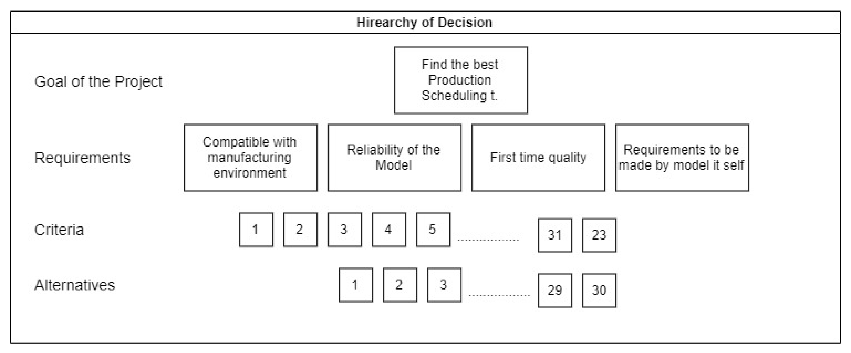
Figure 8 below illustrates the created AHP model. The aim of the project was to find the most suitable real-time scheduling technique that works in Industry 4.0 environments. On the basis of literature analysis, four main requirements were determined:

• Compatibility with manufacturing environment. The model must be in a cyber–physical system system, and communicate with other elements in the manufacturing system.
• Model reliability. The responsible organizations or departments must have access to the model that must be available at any time. The customization feature is also important because every business process is slightly different. A good scheduling technique deals with quality and reduces risk. Therefore, failure-mode and -effect analysis can provide information about possible risks, and makes more reliable decisions.
• First-time quality. First-time quality and other quality features have to be considered.
• Requirements for the model to be developed. Expected outcomes are obtained by using different types of input data, their variety, and the applied algorithm.

Scheduling-Technique Requirements for Selection

The pairwise comparisons of criteria and related subcriteria were performed, and the obtained results are as follows.

Criteria and related subcriteria were pairwise compared, and results were as follows: Criteria: Considering the main criteria, six comparisons were made, and attributes were ranked as: (1) compatibility with the manufacturing environment, (2) reliability, (3) meeting requirements, and (4) first-time quality. The consistency ratio of this ranking was 0.02, as shown in

Table 3. Level 1 criteria.

S/No:	Criteria Level 1	Importance
1	Compatible with manufacturing environment	0.595
2	Reliability	0.245
3	First-time quality	0.071
4	Requirements to be made by model itself	0.089

CR = 0.02.

.

For subcriteria 1, as illustrated in

Table 4. Level 2—subcriteria 1.

S/No:	Level 2 Criteria	Importance
1	Customer demand	0.162
2	Bill of material	0.124
3	Control system	0.028
4	Cycle time of the product	0.041
5	ERP system	0.013
6	Event logs available	0.097
7	Internet of Things (connectedness)	0.072
8	Inventory Level in real time	0.019
9	Monitored production	0.052
10	Resources in real time ( Lab or, Machine)	0.185
11	Sensors and actuators	0.066
12	Takt time of every product	0.142

CR = 0.01.

, comparisons with a consistency ratio of 0.01 were made: resources in real time (labor, machines), ranked 1; customer demand, ranked 2; takt time, ranked 3; bill of material, ranked 4; available event logs, ranked 5; Internet of Things, ranked 6; sensors and actuators, ranked 7; monitored production, ranked 8; cycle time of products, ranked 9; control systems, ranked 10; inventory level in real time, ranked 11; and available ERP system, ranked 12.

For subcriteria 2, as illustrated in

Table 5. Level 2—subcriteria 2.

S/No:	Level 2 Subcriteria 2	Importance
1	Management and organization	0.411
2	References	0.209
3	Customization capability	0.333
4	Communication	0.047

CR = 0.052.

, four comparisons with a consistency ratio of 0.052 were made: management and organization were ranked 1; customization, ranked 2; references, ranked 3; and communication, ranked 4.

For subcriteria 3, as illustrated in

Table 6. Level 2—subcriteria 3.

S/No:	Level 2 Subcriteria 3	Importance
1	Product Variety	0.489
2	Product-quality features	0.444
3	Production quality	0.067

CR = 0.072092.

, three comparisons with a consistency ratio of 0.072092 were made: product variety, ranked 1; product-quality features, ranked 2; and production quality, ranked 3.

For subcriteria 4, as illustrated in

Table 7. Level 2—subcriteria 4.

S/No:	Level 2 Subcriteria 3	Importance
1	Due/finishing date of job	0.076
2	Processing time of each job	0.146
3	Maximal limit of completion time of job. If actual time is longer than planned time, it needs to be rescheduled.	0.083
4	Weight of job (may be sequence of job)	0.049
5	Preparation time for starting production	0.145
6	Number of jobs that are processed	0.11
7	Number of machines	0.051
8	Permutation job setting	0.056
9	Number of orders	0.039
10	Priority of orders	0.05
11	Variance of time needed to process job on a given machine	0.039
12	Waiting time	0.05
13	Walking time of workers	0.04

CR = 0.087616.

, comparisons with a consistency ratio of 0.087616 were made: finishing date of the job, ranked 1; job completion, ranked 2; job weight, ranked 3; job processing time, ranked 4; job duration, ranked 5; number of machines, ranked 6; number of jobs to be processed, ranked 7; variance of job needed to process job/machines; ranked 8; priority of orders, ranked 9; permutation of orders, ranked 10; waiting time, ranked 11; and walking time, ranked 12.

Out of 27 scheduling methods, only seven (hybrid optimization, 81.03%; genetic algorithms, 77.88%; multiagent method, 76.33%; neural networks, 72.97%; simulation methods, 72.86%; expert systems, 70.59%; and tabu search, 69.91%) scored more than 65% and all fell into the category of heuristic scheduling methods as illustrated in

Table 8. Best scheduling alternatives based on AHP analysis.

S/No:	Selected Scheduling Methods	Score in %
1	Hybrid optimization	81.03
2	Genetic algorithms	77.88
3	Multiagent method	76.33
4	Neural network	72.97
5	Simulation methods	72.86
6	Expert system	70.59
7	Tabu search	69.91

. Hybrid optimization (genetic algorithms and multiagent methods) was selected as a model of the decision-support system to be implemented in robotic process automation.

Results in

Table 9. Score results of best selected scheduling methods after AHP analysis.

S/No:	Score Results of Scheduling Methods after AHP Analysis	in %
1	New Hybrid (MB–GA)	83.42
2	Hybrid optimization	82.17
3	Genetic algorithms	78.58
4	Tabu search	76.05
5	Simulation methods	74.39
6	Neural network	72.22
7	Multiagent method	69.54
8	Expert system	57.58

show the scores of each scheduling method after AHP analysis. The new hybrid (MB–GA) scored 83.42%, the highest percentage. The above was accompanied by a hybrid scheduling-optimization technique with a score of 82.17%. The last was an expert system with a ranking of 57.58%.

5. Conclusions

This paper discussed the development of a conceptual real-time decision-support system for high-mix low-volume (HMLV) production scheduling in Industry 4.0 environments. We compared the new MB–GA method with different scheduling techniques to reveal their performance in Industry 4.0 environments. Research was guided by our research questions.

Analysis of the scheduling methods was performed by using the analytical-hierarchy-process tool. Qualitative data were gathered from literature reviews from a variety of scientific sources (journals, scientific articles and papers, studies, books, and other online platforms) and intuitive thinking.

On the basis of guidance of the research questions, 27 scheduling methods were analyzed and grouped into eight categories. Then, more than 17 manufacturing requirements were identified that were later reduced to 12. Subsequently, more than 17 model requirements were identified, and all were left without pruning/uncut; four reliability and three first-time qualities were also identified. Lastly, the AHP method was used to select the best alternative from the four categories of attributes, and compare the new developed method with others existing in the literature.

The real-time decision-support system model for production scheduling in Industry 4.0 environments that is to be implemented under Industry 4.0 stands to be the best global minimal total makespan and—when implemented in RPA environments—offers a predominant/significant reduction of rescheduling time by more than 50%, and accuracy by more than 90%.

According to the survey results, 16% of the companies can implement the new method, and an additional 43.2% can deal with the risks. Consequently, if they collect and measure the required parameters, they can implement the new method as well. However, this requires and induces a little modification in production. This modification creates an environment to collect and store historical data about the production that are required for tcFMEA.

The GA searches a population of points, not a single point. Intrinsically parallel to the population level, genetic algorithms are scanned. It can also avoid being stuck by conventional solutions from one point of the local solution. The GA is used in classification and optimization of data mining.

The MB–GA scheduling method involves the mutation operator by adding a randomly generated number to individual population parameters. This means that there are no exact controllers in MB–GA, but probability rules are used, and the method is computationally expensive.

At the end of the paper, answers to the research questions are stated:

• a. What kind of scheduling methods are available for HMLV manufacturing systems?
  b. What kind of scheduling methods can be applied in the field of digitalized manufacturing?
  If attributes of Industry 4.0 are considered, the best technique is the new MG–GA scheduling method. It is flexible and easy to automate, and not industry-specific because it uses general KPIs and parameters. It has a little advantage ahead of hybrid optimization, and a massive advantage in respect of the general GA or tabu search. The list about the most suitable scheduling methods can be seen in Table 9.
• What kind of requirements are stated for scheduling in the field of digitalized manufacturing?
  The list of requirements can be seen in Table 3, Table 4, Table 5, Table 6 and Table 7. The most important is available resources in real time, after customer demands. It is not possible to produce anything without resources and without every customer demand delivered, which is why resources are ahead of customer demand. However, in HMLV production, product variety is high, so there is the possibility to customize by customer.
• Can we create a real-time decision-making environment with the use of RPA?
  The process model of the developed concept can be seen in Figure 5 and Figure 6.

References

- Araya, J.M. Value Stream Mapping Adapted to High-Mix, Low-Volume Manufacturing Environments. Master’s Thesis, KTH Royal Institute of Technology, Stockholm, Sweden, 2012. [Google Scholar]
- Neoh, S.C.; Morad, N.; Lim, C.P.; Aziz, Z.A. A Layered-Encoding Cascade Optimization Approach to Product-Mix Planning in High-Mix–Low-Volume Manufacturing. IEEE Trans. Syst. Man Cybern. Part A Syst. Hum. 2009, 40, 133–146. [Google Scholar] [CrossRef]
- Becker, J.M.J.; Borst, J.; van der Veen, A. Improving the overall equipment effectiveness in high-mix- low-volume manufacturing environments. CIRP Ann. 2015, 64, 419–422. [Google Scholar] [CrossRef]
- Veerakamolmal, P.; Gupta, S.M. High-mix/low-volume batch of electronic equipment disassembly. Comput. Ind. Eng. 1998, 35, 65–68. [Google Scholar] [CrossRef]
- Katragjini, K.; Vallada, E.; Ruiz, R. Flow shop rescheduling under different types of disruption. Int. J. Prod. Res. 2013, 51, 780–797. [Google Scholar] [CrossRef]
- Metaxiotis, K.S.; Psarras, J.E.; Ergazakis, K.A. Production scheduling in ERP systems: An AI-based approach to face the gap. Bus. Process. Manag. J. 2003, 9, 221–247. [Google Scholar] [CrossRef]
- Jain, A.K.; Elmaraghy, H.A. Production scheduling/rescheduling in flexible manufacturing. Int. J. Prod. Res. 1997, 35, 281–309. [Google Scholar] [CrossRef]
- Sule, D.R. Production Planning and Industrial Scheduling: Examples, Case Studies and Applications; CRC Press: Boca Raton, FL, USA, 2007. [Google Scholar]
- Azemi, F.; Šimunović, G.; Lujić, R.; Tokody, D. Intelligent Computer-Aided resource planning and scheduling of machining operation. Procedia Manuf. 2019, 32, 331–338. [Google Scholar] [CrossRef]
- Minguillon, F.E.; Lanza, G. Coupling of centralized and decentralized scheduling for robust production in agile production systems. Procedia CIRP 2019, 79, 385–390. [Google Scholar] [CrossRef]
- Zhong, R.Y.; Xu, X.; Klotz, E.; Newman, S.T. Intelligent Manufacturing in the Context of Industry 4.0: A Review. Engineering 2017, 3, 616–630. [Google Scholar] [CrossRef]
- Ribeiro da Silva, E.H.D.; Angelis, J.; de Lima, E.P. In pursuit of Digital Manufacturing. Procedia Manuf. 2019, 28, 63–69. [Google Scholar] [CrossRef]
- Ribeiro da Silva, E.H.D.; Shinohara, A.C.; de Lima, E.P.; Angelis, J.; Machado, C.G. Reviewing Digital Manufacturing concept in the Industry 4.0 paradigm. Procedia CIRP 2019, 81, 240–245. [Google Scholar] [CrossRef]
- Gregori, F.; Papetti, A.; Pandolfi, M.; Peruzzini, M.; Germani, M. Digital Manufacturing Systems: A Framework to Improve Social Sustainability of a Production Site. Procedia CIRP 2017, 63, 436–442. [Google Scholar] [CrossRef]
- Machado, C.G.; Winroth, M.; Carlsson, D.; Almström, P.; Centerholt, V.; Hallin, M. Industry 4.0 readiness in manufacturing companies: Challenges and enablers towards increased digitalization. Procedia CIRP 2019, 81, 1113–1118. [Google Scholar] [CrossRef]
- Monostori, L.; Kádár, B.; Bauernhansl, T.; Kondoh, S.; Kumara, S.; Reinhart, G.; Sauer, O.; Schuh, G.; Sihn, W.; Ueda, K. Cyber-physical systems in manufacturing. CIRP Ann. 2016, 65, 621–641. [Google Scholar] [CrossRef]
- Meissner, H.; Aurich, J.C. Implications of Cyber-Physical Production Systems on Integrated Process Planning and Scheduling. Procedia Manuf. 2019, 28, 167–173. [Google Scholar] [CrossRef]
- Rossit, D.A.; Tohmé, F.; Frutos, M. Industry 4.0: Smart Scheduling. Int. J. Prod. Res. 2019, 57, 3802–3813. [Google Scholar] [CrossRef]
- Elazouni, A. Heuristic method for multi-project finance-based scheduling. Constr. Manag. Econ. 2009, 27, 199–211. [Google Scholar] [CrossRef]
- Schulte, J.; Becker, B.D. Production scheduling using genetic algorithms. In Information Control Problems in Manufacturing Technology 1992; Elsevier: Amsterdam, The Netherlands, 1993; pp. 367–372. [Google Scholar]
- Teekeng, W.; Thammano, A. Modified Genetic Algorithm for Flexible Job-Shop Scheduling Problems. Procedia Comput. Sci. 2012, 12, 122–128. [Google Scholar] [CrossRef]
- Liu, X.; Wang, L.; Kong, L.; Li, F.; Li, J. A Hybrid Genetic Algorithm for Minimizing Energy Consumption in Flow Shops Considering Ultra-low Idle State. Procedia CIRP 2019, 80, 192–196. [Google Scholar] [CrossRef]
- Tayeb, F.B.S.; Bessedik, M.; Benbouzid, M.; Cheurfi, H.; Blizak, A. Research on Permutation Flow-shop Scheduling Problem based on Improved Genetic Immune Algorithm with vaccinated offspring. Procedia Comput. Sci. 2017, 112, 427–436. [Google Scholar] [CrossRef]
- Zhang, R.; Chang, P.C.; Wu, C. A hybrid genetic algorithm for the job shop scheduling problem with practical considerations for manufacturing costs: Investigations motivated by vehicle production. Int. J. Prod. Econ. 2013, 145, 38–52. [Google Scholar] [CrossRef]
- Ak, B.; Koc, E. A Guide for Genetic Algorithm Based on Parallel Machine Scheduling and Flexible Job-Shop Scheduling. Procedia Soc. Behav. Sci. 2012, 62, 817–823. [Google Scholar] [CrossRef][Green Version]
- Azzouz, A.; Ennigrou, M.; Said, L.B. A self-adaptive hybrid algorithm for solving flexible job-shop problem with sequence dependent setup time. Procedia Comput. Sci. 2017, 112, 457–466. [Google Scholar] [CrossRef]
- Grosch, B.; Weitzel, T.; Panten, N.; Abele, E. A metaheuristic for energy adaptive production scheduling with multiple energy carriers and its implementation in a real production system. Procedia CIRP 2019, 80, 203–208. [Google Scholar] [CrossRef]
- Thammano, A.; Teekeng, W. A modified genetic algorithm with fuzzy roulette wheel selection for job-shop scheduling problems. Int. J. Gen. Syst. 2015, 44, 499–518. [Google Scholar] [CrossRef]
- Mohan, J.; Lanka, K.; Rao, A.N. A Review of Dynamic Job Shop Scheduling Techniques. Procedia Manuf. 2019, 30, 34–39. [Google Scholar] [CrossRef]
- Nowicki, E.; Smutnicki, C. New results in the worst-case analysis for flow-shop scheduling. Discret. Appl. Math. 1993, 46, 21–41. [Google Scholar] [CrossRef][Green Version]
- De Carvalho, M.F.G.; Haddad, R.B.B. Production scheduling on practical problems. In Production Scheduling; InTech: Rijeka, Croatia, 2012; pp. 157–182. [Google Scholar]
- Tang, J.; Zhang, G.; Lin, B.; Zhang, B. A Hybrid Algorithm for Flexible Job-Shop Scheduling Problem. Procedia Eng. 2011, 15, 3678–3683. [Google Scholar] [CrossRef]
- Lin, L.; Gen, M.; Liang, Y.; Ohno, K. A Hybrid EA for Reactive Flexible Job-shop Scheduling. Procedia Comput. Sci. 2012, 12, 110–115. [Google Scholar] [CrossRef]
- Ahmad, I.; Ayub, A.; Kano, M.; Cheema, I.I. Gray-box Soft Sensors in Process Industry: Current Practice, and Future Prospects in Era of Big Data. Processes 2020, 8, 243. [Google Scholar] [CrossRef]
- Henning, K. Recommendations for Implementing the Strategic Initiative INDUSTRIE 4.0; Acatech: Munich, Germany, 2013. [Google Scholar]
- Bogle, I.D.L. A Perspective on Smart Process Manufacturing Research Challenges for Process Systems Engineers. Engineering 2017, 3, 161–165. [Google Scholar] [CrossRef]
- Waibel, M.W.; Steenkamp, L.P.; Moloko, N.; Oosthuizen, G.A. Investigating the Effects of Smart Production Systems on Sustainability Elements. Procedia Manuf. 2017, 8, 731–737. [Google Scholar] [CrossRef]
- Laudante, E. Industry 4.0, Innovation and Design. A new approach for ergonomic analysis in manufacturing system. Des. J. 2017, 20, S2724–S2734. [Google Scholar] [CrossRef]
- Billaut, J.C.; Roubellat, F. A new method for workshop real time scheduling. Int. J. Prod. Res. 1996, 34, 1555–1579. [Google Scholar] [CrossRef]
- Billaut, J.C.; Roubellat, F. Characterization of a set of schedules in a multiple resource context. J. Decis. Syst. 1996, 5, 95–109. [Google Scholar] [CrossRef]
- Akkan, C. Overtime Scheduling: An Application in Finite-Capacity Real-Time Scheduling. J. Oper. Res. Soc. 1996, 47, 1137–1149. [Google Scholar] [CrossRef]
- Vafeiadis, T.; Kalatzis, D.; Nizamis, A.; Ioannidis, D.; Apostolou, K.; Metaxa, I.; Charisi, V.; Beecks, C.; Insolvibile, G.; Pardi, M. Data analysis and visualization framework in the manufacturing decision support system of COMPOSITION project. Procedia Manuf. 2019, 28, 57–62. [Google Scholar] [CrossRef]
- Chang, W.Y.; Tsai, W.F.; Lai, J.S.; Wu, J.H.; Lien, H.C.; Chung, T.L.; Shiau, Y.H.; Liao, Y.H.; Lin, F.P. Development of a real-time monitoring system as a decision-support system for flood hazard mitigation. J. Chin. Inst. Eng. 2012, 35, 827–840. [Google Scholar] [CrossRef]
- Van der Aalst, W.M.; Bichler, M.; Heinzl, A. Robotic Process Automation. Bus. Inf. Syst. Eng. 2018, 60, 269–272. [Google Scholar] [CrossRef]
- Kirchmer, M.; Robotic Process Automation-Pragmatic Solution or Dangerous Illusion. BTOES Insights 2017. Available online: https://insights.btoes.com/risks-robotic-process-automation-pragmatic-solution-or-dangerous-illusion (accessed on 28 July 2020).
- Willcocks, L.P.; Lacity, M.; Craig, A. The IT Function and Robotic Process Automation; The London School of Economics and Political Science: London, UK, 2015. [Google Scholar]
- Neelakandan, S.; Tyagi, A.; Nagalkar, D. Robotic Process Automation for Supply Chain Management Operations. U.S. Patent 10,324,457, 18 June 2019. [Google Scholar]
- Hall, S.; Schiopu, V.; van den Heuvel, J.; Jacquot, A. Self-Learning Robotic Process Automation. US Patent US20190265990A1, 5 March 2019. [Google Scholar]
- Petersen, B.L.; Rohith, G.P. How Robotic Process Automation and Artificial Intelligence Will Change Outsourcing; Mayer Brown: Brussels, Belgium, 2017. [Google Scholar]
- Lacity, M.; Willcocks, L.P.; Craig, A. Robotic Process Automation at Telefonica O2; The London School of Economics and Political Science: London, UK, 2015. [Google Scholar]
- Asatiani, A.; Penttinen, E. Turning robotic process automation into commercial success–Case OpusCapita. J. Inf. Technol. Teach. Cases 2016, 6, 67–74. [Google Scholar] [CrossRef]
- Lacity, M.; Willcocks, L. Robotic process automation: The next transformation lever for shared services. Lond. Sch. Econ. Outsourcing Unit Work. Pap. 2015, 7, 1–35. [Google Scholar]
- Willcocks, L.; Lacity, M.; Craig, A. Robotic process automation: Strategic transformation lever for global business services? J. Inf. Technol. Teach. Cases 2017, 7, 17–28. [Google Scholar] [CrossRef]
- Hastings, N.A.; Yeh, C.H. Bill of manufacture. Prod. Inventory Manag. J. 1992, 33, 27. [Google Scholar]
- Rahani, A.R.; Al Ashraf, M. Production Flow Analysis through Value Stream Mapping: A Lean Manufacturing Process Case Study. Procedia Eng. 2012, 41, 1727–1734. [Google Scholar] [CrossRef]
- Linck, J.; Cochran, D.S. The Importance of Takt Time in Manufacturing System Design; SAE Technical Paper; SAE International: Warrendale, PA, USA, 1999. [Google Scholar]
- Sundar, R.; Balaji, A.; Kumar, R.S. A review on lean manufacturing implementation techniques. Procedia Eng. 2014, 97, 1875–1885. [Google Scholar] [CrossRef]
- Der Aalst, W.V.; Weijters, T.; Maruster, L. Workflow mining: Discovering process models from event logs. IEEE Trans. Knowl. Data Eng. 2004, 16, 1128–1142. [Google Scholar] [CrossRef]
- Rozinat, A.; Van der Aalst, W.M. Conformance testing: Measuring the fit and appropriateness of event logs and process models. In Proceedings of the International Conference on Business Process Management, Nancy, France, 5 September 2005; Springer: Berlin/Heidelberg, Germany; pp. 163–176.
- Song, M.; Günther, C.W.; Van der Aalst, W.M. Trace clustering in process mining. In Proceedings of the International Conference on Business Process Management, Milano, Italy, 1–4 September 2008; Springer: Berlin/Heidelberg, Germany; pp. 109–120.
- Xia, F.; Yang, L.T.; Wang, L.; Vinel, A. Internet of things. Int. J. Commun. Syst. 2012, 25, 1101. [Google Scholar] [CrossRef]
- Sassi, M.S.H.; Jedidi, F.G.; Fourati, L.C. A New Architecture for Cognitive Internet of Things and Big Data. Procedia Comput. Sci. 2019, 159, 534–543. [Google Scholar] [CrossRef]
- Kurebwa, J.G.; Mushiri, T. Internet of things architecture for a smart passenger-car robotic first aid system. Procedia Manuf. 2019, 35, 27–34. [Google Scholar] [CrossRef]
- Zhou, Y.; Wang, K.; Liu, H. An Elevator Monitoring System Based on the Internet of Things. Procedia Comput. Sci. 2018, 131, 541–544. [Google Scholar] [CrossRef]
- Boyes, H.; Hallaq, B.; Cunningham, J.; Watson, T. The industrial internet of things (IIoT): An analysis framework. Comput. Ind. 2018, 101, 271439. [Google Scholar] [CrossRef]
- Schmitt, G.; Mladenow, A.; Strauss, C.; Schaffhauser-Linzatti, M. Smart Contracts and Internet of Things: A Qualitative Content Analysis using the Technology-Organization-Environment Framework to Identify Key-Determinants. Procedia Comput. Sci. 2019, 160, 189–196. [Google Scholar] [CrossRef]
- Allhoff, F.; Henschke, A. The Internet of Things: Foundational ethical issues. Internet Things 2018, 1–2, 55–66. [Google Scholar] [CrossRef]
- Jose, D.V.; Vijyalakshmi, A. An Overview of Security in Internet of Things. Procedia Comput. Sci. 2018, 143, 744–748. [Google Scholar] [CrossRef]
- Brous, P.; Janssen, M.; Herder, P. The dual effects of the Internet of Things (IoT): A systematic review of the benefits and risks of IoT adoption by organizations. Int. J. Inf. Manag. 2019, 51, 101952. [Google Scholar] [CrossRef]
- Ray, P.P. A survey on Internet of Things architectures. J. King Saud Univ. Comput. Inf. Sci. 2018, 30, 291–319. [Google Scholar] [CrossRef]
- Gupta, A.K.; Souder, W.E. Key drivers of reduced cycle time. Res. Technol. Manag. 1998, 41, 38–43. [Google Scholar] [CrossRef]
- Georgiadis, P.; Michaloudis, C. Real-time production planning and control system for job-shop manufacturing: A system dynamics analysis. Eur. J. Oper. Res. 2012, 216, 94–104. [Google Scholar] [CrossRef]
- DePuy, G.; Usher, J.; Walker, R.; Taylor, G. Production planning for remanufactured products. Prod. Plan. Control 2007, 18, 573–583. [Google Scholar] [CrossRef]
- Madanhire, I.; Mbohwa, C. Enterprise Resource Planning (ERP) in Improving Operational Efficiency: Case Study. Procedia CIRP 2016, 40, 225–229. [Google Scholar] [CrossRef]
- Shen, Y.C.; Chen, P.S.; Wang, C.H. A study of enterprise resource planning (ERP) system performance measurement using the quantitative balanced scorecard approach. Comput. Ind. 2016, 75, 127–139. [Google Scholar] [CrossRef]
- Hsu, L.L.; Chen, M. Impacts of ERP systems on the integrated-interaction performance of manufacturing and marketing. Ind. Manag. Data Syst. 2004, 104, 42–55. [Google Scholar] [CrossRef]
- Tarantilis, C.D.; Kiranoudis, C.T.; Theodorakopoulos, N.D. A Web-based ERP system for business services and supply chain management: Application to real-world process scheduling. Eur. J. Oper. Res. 2008, 187, 1310–1326. [Google Scholar] [CrossRef]
- Palaniswamy, R.; Frank, T. Enhancing manufacturing performance with ERP systems. Inf. Syst. Manag. 2000, 17, 43–55. [Google Scholar] [CrossRef]
- Chen, I.J. Planning for ERP systems: Analysis and future trend. Bus. Process. Manag. J. 2001, 7, 374–386. [Google Scholar] [CrossRef]
- Canelas, E.; Pinto-Varela, T.S.B. Electricity Portfolio Optimization for Large Consumers: Iberian Electricity Market Case Study. Energies 2020, 13, 2249. [Google Scholar] [CrossRef]
- Abusalem, O.; Bertalan, N.; Kocsi, B. Implementing quantitative techniques to improve decision making in construction projects: A case study. Pollack Period. 2019, 14, 223–234. [Google Scholar] [CrossRef]
- Schwalbe, K. An Introduction to Project Management; CreateSpace: North Charleston, NC, USA, 2017. [Google Scholar]
- Rosen, R.; Von Wichert, G.; Lo, G.; Bettenhausen, K.D. About The Importance of Autonomy and Digital Twins for the Future of Manufacturing. IFAC PapersOnLine 2015, 48, 567–572. [Google Scholar] [CrossRef]
- Hulett, D.T. Practical Schedule Risk Analysis; Gower Publishing, Ltd.: Aldershot, UK, 2009. [Google Scholar]
- Lewandowska-Ciszek, A. Complexity of a modern enterprise and its flexibility in the sector of industrial automation. Bull. Pol. Acad. Sci. Tech. Sci. 2020, 68, 575–584. [Google Scholar] [CrossRef]
- Banduka, N.; Veza, I.; Bilić, B. An integrated lean approach to Process Failure Mode and Effect Analysis (PFMEA): A case study from automotive industry. Adv. Prod. Eng. Manag. 2016. [Google Scholar] [CrossRef]
- Montgomery, T.A.; Marko, K.A. Quantitative FMEA automation. In Proceedings of the Annual Reliability and Maintainability Symposium, Philadelphia, PA, USA, 13–16 January 1997. [Google Scholar]
© 2020 by the authors. Licensee MDPI, Basel, Switzerland. This article is an open access article distributed under the terms and conditions of the Creative Commons Attribution (CC BY) license (http://creativecommons.org/licenses/by/4.0/).