Measuring Performance Metrics of Machine Learning Algorithms for Detecting and Classifying Transposable Elements

 ,
,  ,
,  and
and 
Abstract
1. Introduction
2. Materials and Methods
2.1. Bibliography Analysis
2.2. Measure Invariance Analysis
- Exchange of positives and negatives (I1): A measure presents invariance in this property if showing invariance corresponding to the distribution of classification results due to its inability to differentiate tp from tn and fn from fp. An invariant metric in this property may not be utilized in datasets highly unbalanced [40], such as the number of TEs belonging to each lineage in the Repbase or PGSB databases.
- Change of true negative counts (I2): A measure presents invariance in this property if , demonstrating the inability to recognize specificity of the classifiers. This property can be useful in problems with multi-modal negative class (the class with all elements other than the positive), i.e., in the detection of TEs, where negative class may be composed by all other genomic features such as genes, CDS (coding sequences), and simple repeats, among others.
- Change of true positive counts (I3): A measure presents invariance in this property if , losing the sensitivity of the classifiers, so their evaluation should be complementary to other metrics.
- Change of false negative counts (I4): A measure presents invariance in this property if , indicating stability even when the classifier has errors assigning negative labels. It is helpful in detecting or classifying TEs when non-curated databases are used in training (such as RepetDB), which may contain mistakes.
- Change of false positive counts (I5): A measure presents invariance in this property if , proving reliable results even though some classes contain outliers, which is common in elements classified at lineage level due to TE diversity in their nucleotide sequences [26].
- Uniform change of positives and negatives (I6): A measure presents invariance in this property if , with It indicates if a measure’s value changes when the size of the dataset increases. The non-invariance indicates that the application of the metric depends on size of the data.
- Change of positive and negative columns (I7): A measure presents invariance in this property if , with If a metric is unchanged in this way, it will not show changes when additional datasets differs from training datasets in quality (i.e., having more noise), and indicating the needed of other measures as complement. On the contrary, if a metric presents a non-invariant behavior then, it may be suitable if different performances are expected across classes.
- Change of positive and negative rows (I8): A measure presents invariance in this property if , with In this case, if a metric is non-invariant, its applicability depends on the quality of the classes. It may be useful, for example, when curated datasets are available such as Repbase.
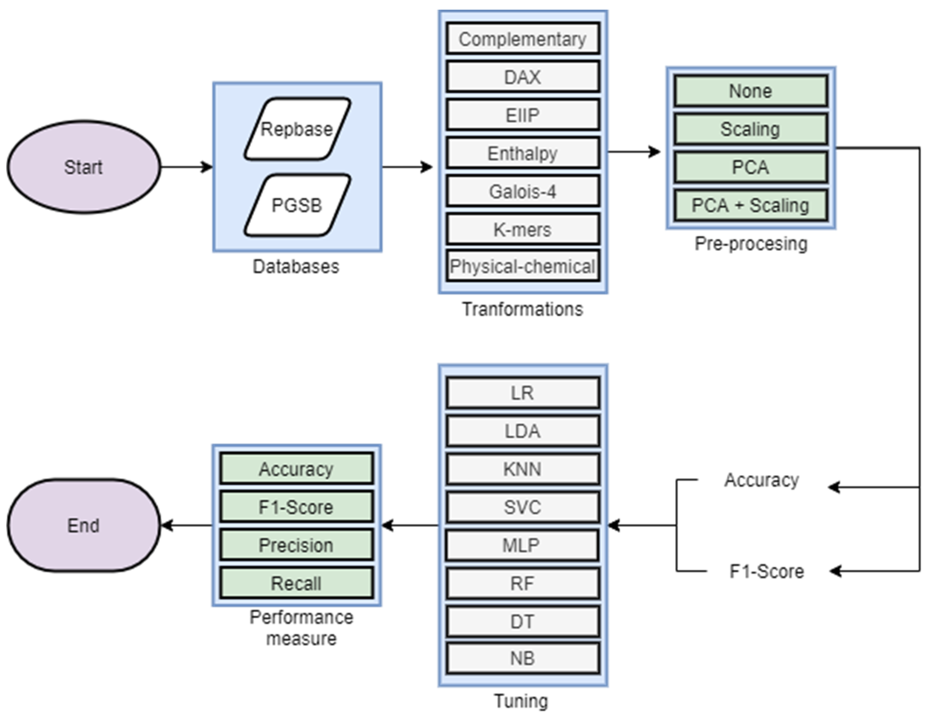
2.3. Experimental Analysis
3. Results
3.1. Bibliography and Invariance Analysis
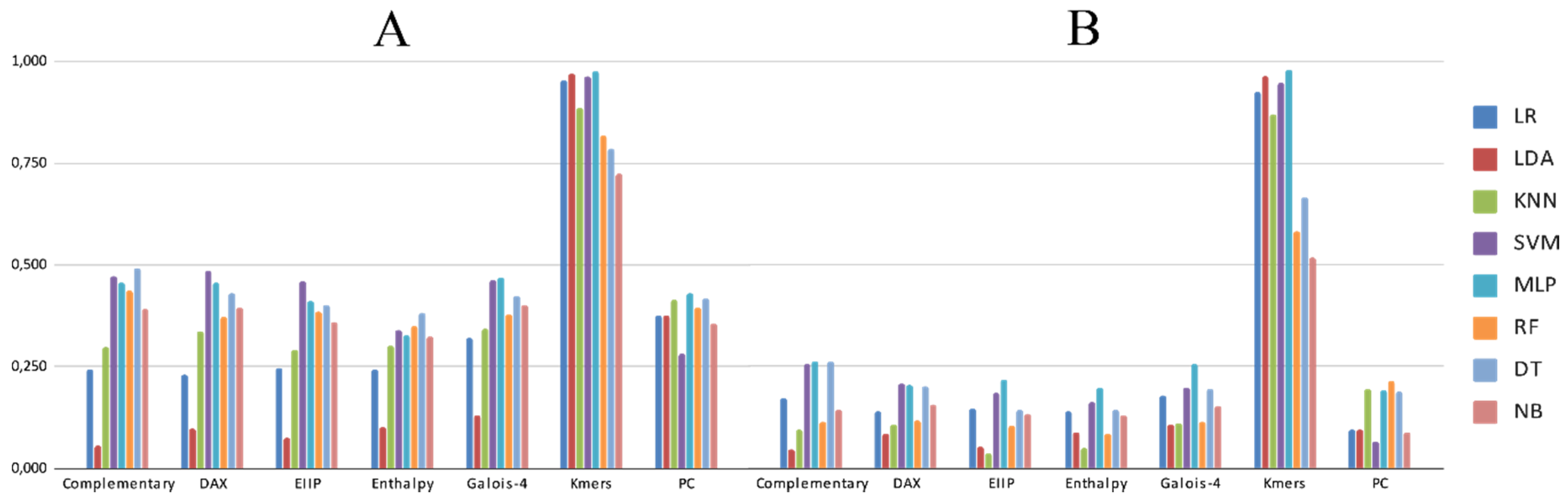
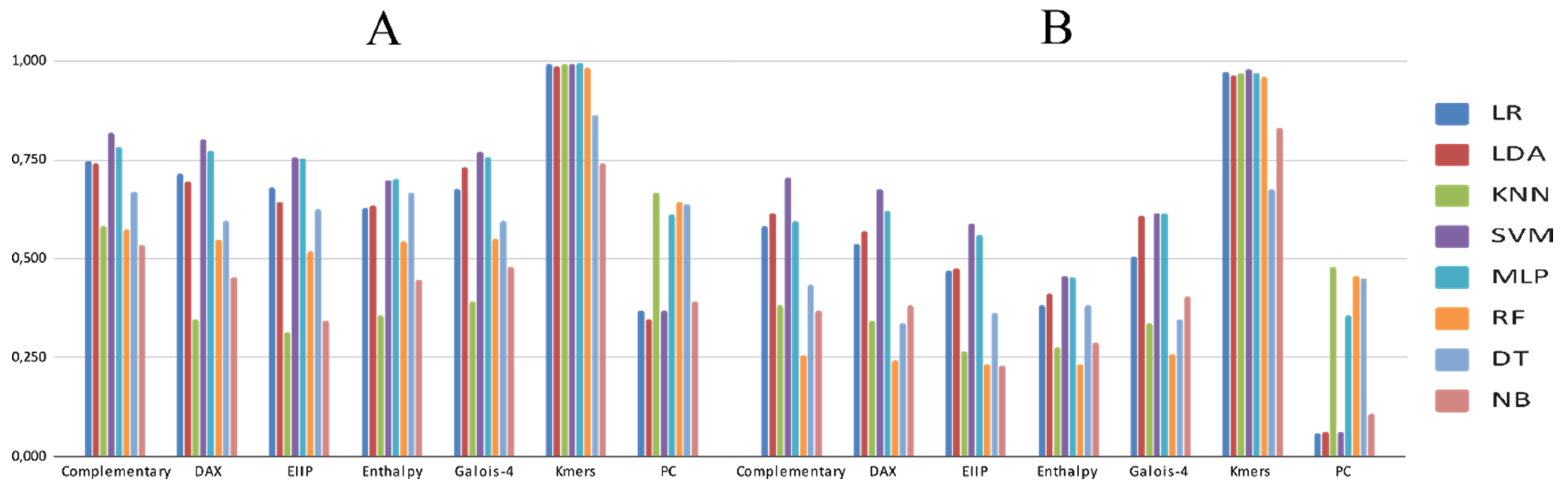
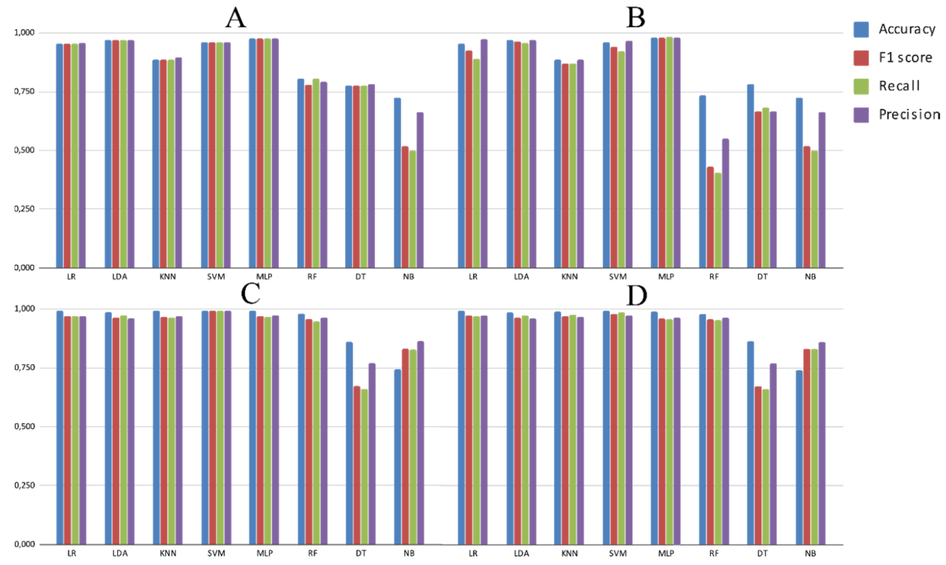
3.2. Experimental Analysis
4. Discussion
5. Conclusions
Supplementary Materials
Author Contributions
Funding
Acknowledgments
Conflicts of Interest
References
- Mita, P.; Boeke, J.D. How retrotransposons shape genome regulation. Curr. Opin. Genet. Dev. 2016, 37, 90–100. [Google Scholar] [CrossRef] [PubMed]
- Keidar, D.; Doron, C.; Kashkush, K. Genome-wide analysis of a recently active retrotransposon, Au SINE, in wheat: Content, distribution within subgenomes and chromosomes, and gene associations. Plant Cell Rep. 2018, 37, 193–208. [Google Scholar] [CrossRef] [PubMed]
- Orozco-Arias, S.; Isaza, G.; Guyot, R. Retrotransposons in Plant Genomes: Structure, Identification, and Classification through Bioinformatics and Machine Learning. Int. J. Mol. Sci. 2019, 20, 781. [Google Scholar] [CrossRef] [PubMed]
- De Castro Nunes, R.; Orozco-Arias, S.; Crouzillat, D.; Mueller, L.A.; Strickler, S.R.; Descombes, P.; Fournier, C.; Moine, D.; de Kochko, A.; Yuyama, P.M.; et al. Structure and Distribution of Centromeric Retrotransposons at Diploid and Allotetraploid Coffea Centromeric and Pericentromeric Regions. Front. Plant Sci. 2018, 9, 175. [Google Scholar] [CrossRef] [PubMed]
- Ou, S.; Chen, J.; Jiang, N. Assessing genome assembly quality using the LTR Assembly Index (LAI). Nucleic Acids Res. 2018, 1–11. [Google Scholar] [CrossRef] [PubMed]
- Mustafin, R.N.; Khusnutdinova, E.K. The Role of Transposons in Epigenetic Regulation of Ontogenesis. Russ. J. Dev. Biol. 2018, 49, 61–78. [Google Scholar] [CrossRef]
- Chaparro, C.; Gayraud, T.; De Souza, R.F.; Domingues, D.S.; Akaffou, S.S.; Vanzela, A.L.L.; De Kochko, A.; Rigoreau, M.; Crouzillat, D.; Hamon, S.; et al. Terminal-repeat retrotransposons with GAG domain in plant genomes: A new testimony on the complex world of transposable elements. Genome Biol. Evol. 2015, 7, 493–504. [Google Scholar] [CrossRef]
- Wicker, T.; Sabot, F.; Hua-Van, A.; Bennetzen, J.L.; Capy, P.; Chalhoub, B.; Flavell, A.; Leroy, P.; Morgante, M.; Panaud, O.; et al. A unified classification system for eukaryotic transposable elements. Nat. Rev. Genet. 2007, 8, 973–982. [Google Scholar] [CrossRef]
- Neumann, P.; Novák, P.; Hoštáková, N.; MacAs, J. Systematic survey of plant LTR-retrotransposons elucidates phylogenetic relationships of their polyprotein domains and provides a reference for element classification. Mob. DNA 2019, 10, 1–17. [Google Scholar] [CrossRef]
- Loureiro, T.; Camacho, R.; Vieira, J.; Fonseca, N.A. Improving the performance of Transposable Elements detection tools. J. Integr. Bioinform. 2013, 10, 231. [Google Scholar] [CrossRef] [PubMed][Green Version]
- Nakano, F.K.; Mastelini, S.M.; Barbon, S.; Cerri, R. Improving Hierarchical Classification of Transposable Elements using Deep Neural Networks. In Proceedings of the Proceedings of the International Joint Conference on Neural Networks, Rio de Janeiro, Brazil, 8–13 July 2018; Volume 8–13 July. [Google Scholar]
- Lewin, H.A.; Robinson, G.E.; Kress, W.J.; Baker, W.J.; Coddington, J.; Crandall, K.A.; Durbin, R.; Edwards, S.V.; Forest, F.; Gilbert, M.T.P.; et al. Earth BioGenome Project: Sequencing life for the future of life. Proc. Natl. Acad. Sci. USA 2018, 115, 4325–4333. [Google Scholar] [CrossRef]
- Orozco-arias, S.; Isaza, G.; Guyot, R.; Tabares-soto, R. A systematic review of the application of machine learning in the detection and classi fi cation of transposable elements. PeerJ 2019, 7, 18311. [Google Scholar] [CrossRef] [PubMed]
- Jurka, J.; Kapitonov, V.V.; Pavlicek, A.; Klonowski, P.; Kohany, O.; Walichiewicz, J. Repbase Update, a database of eukaryotic repetitive elements. Cytogenet. Genome Res. 2005, 110, 462–467. [Google Scholar] [CrossRef] [PubMed]
- Cornut, G.; Choisne, N.; Alaux, M.; Alfama-Depauw, F.; Jamilloux, V.; Maumus, F.; Letellier, T.; Luyten, I.; Pommier, C.; Adam-Blondon, A.-F.; et al. RepetDB: A unified resource for transposable element references. Mob. DNA 2019, 10, 6. [Google Scholar]
- Wicker, T.; Matthews, D.E.; Keller, B. TREP: A database for Triticeae repetitive elements 2002. Available online: http://botserv2.uzh.ch/kelldata/trep-db/pdfs/2002_TIPS.pdf (accessed on 24 May 2020).
- Spannagl, M.; Nussbaumer, T.; Bader, K.C.; Martis, M.M.; Seidel, M.; Kugler, K.G.; Gundlach, H.; Mayer, K.F.X. PGSB PlantsDB: Updates to the database framework for comparative plant genome research. Nucleic Acids Res. 2015, 44, D1141–D1147. [Google Scholar] [CrossRef] [PubMed]
- Du, J.; Grant, D.; Tian, Z.; Nelson, R.T.; Zhu, L.; Shoemaker, R.C.; Ma, J. SoyTEdb: A comprehensive database of transposable elements in the soybean genome. BMC Genom. 2010, 11, 113. [Google Scholar] [CrossRef]
- Llorens, C.; Futami, R.; Covelli, L.; Domínguez-Escribá, L.; Viu, J.M.; Tamarit, D.; Aguilar-Rodríguez, J.; Vicente-Ripolles, M.; Fuster, G.; Bernet, G.P.; et al. The Gypsy Database (GyDB) of Mobile Genetic Elements: Release 2.0. Nucleic Acids Res. 2011, 39, 70–74. [Google Scholar] [CrossRef]
- Pedro, D.L.F.; Lorenzetti, A.P.R.; Domingues, D.S.; Paschoal, A.R. PlaNC-TE: A comprehensive knowledgebase of non-coding RNAs and transposable elements in plants. Database 2018, 2018, bay078. [Google Scholar] [CrossRef]
- Lorenzetti, A.P.R.; De Antonio, G.Y.A.; Paschoal, A.R.; Domingues, D.S. PlanTE-MIR DB: A database for transposable element-related microRNAs in plant genomes. Funct. Integr. Genom. 2016, 16, 235–242. [Google Scholar] [CrossRef]
- Kamath, U.; De Jong, K.; Shehu, A. Effective automated feature construction and selection for classification of biological sequences. PLoS ONE 2014, 9, e99982. [Google Scholar] [CrossRef]
- Nakano, F.K.; Martiello Mastelini, S.; Barbon, S.; Cerri, R. Stacking methods for hierarchical classification. In Proceedings of the 16th IEEE International Conference on Machine Learning and Applications, Cancun, Mexico, 18–21 December 2017; Volume 2018–Janua, pp. 289–296. [Google Scholar]
- Nakano, F.K.; Pinto, W.J.; Pappa, G.L.; Cerri, R. Top-down strategies for hierarchical classification of transposable elements with neural networks. In Proceedings of the Proceedings of the International Joint Conference on Neural Networks, Anchorage, AK, USA, 14–19 May 2017; Volume 2017-May, pp. 2539–2546. [Google Scholar]
- Ventola, G.M.M.; Noviello, T.M.R.; D’Aniello, S.; Spagnuolo, A.; Ceccarelli, M.; Cerulo, L. Identification of long non-coding transcripts with feature selection: A comparative study. BMC Bioinform. 2017, 18, 187. [Google Scholar] [CrossRef] [PubMed]
- Rawal, K.; Ramaswamy, R. Genome-wide analysis of mobile genetic element insertion sites. Nucleic Acids Res. 2011, 39, 6864–6878. [Google Scholar] [CrossRef] [PubMed]
- Zamith Santos, B.; Trindade Pereira, G.; Kenji Nakano, F.; Cerri, R. Strategies for selection of positive and negative instances in the hierarchical classification of transposable elements. In Proceedings of the Proceedings - 2018 Brazilian Conference on Intelligent Systems, Sao Paulo, Brazil, 22–25 October 2018; pp. 420–425. [Google Scholar]
- Larrañaga, P.; Calvo, B.; Santana, R.; Bielza, C.; Galdiano, J.; Inza, I.; Lozano, J.A.; Armañanzas, R.; Santafé, G.; Pérez, A.; et al. Machine learning in bioinformatics. Brief. Bioinform. 2006, 7, 86–112. [Google Scholar] [CrossRef]
- Mjolsness, E.; DeCoste, D. Machine learning for science: State of the art and future prospects. Science (80-.) 2001, 293, 2051–2055. [Google Scholar] [CrossRef] [PubMed]
- Libbrecht, M.W.; Noble, W.S. Machine learning applications in genetics and genomics. Nat. Rev. Genet. 2015, 16, 321–332. [Google Scholar] [CrossRef] [PubMed]
- Ceballos, D.; López-álvarez, D.; Isaza, G.; Tabares-Soto, R.; Orozco-Arias, S.; Ferrin, C.D. A Machine Learning-based Pipeline for the Classification of CTX-M in Metagenomics Samples. Processes 2019, 7, 235. [Google Scholar] [CrossRef]
- Loureiro, T.; Camacho, R.; Vieira, J.; Fonseca, N.A. Boosting the Detection of Transposable Elements Using Machine Learning. In 7th International Conference on Practical Applications of Computational Biology & Bioinformatics; Springer: Heidelberg, Germany, 2013; pp. 85–91. [Google Scholar]
- Santos, B.Z.; Cerri, R.; Lu, R.W. A New Machine Learning Dataset for Hierarchical Classification of Transposable Elements. In Proceedings of the XIII Encontro Nacional de Inteligência Artificial-ENIAC, Sao Paulo, Brazil, 9–12 October 2016. [Google Scholar]
- Schietgat, L.; Vens, C.; Cerri, R.; Fischer, C.N.; Costa, E.; Ramon, J.; Carareto, C.M.A.; Blockeel, H. A machine learning based framework to identify and classify long terminal repeat retrotransposons. PLoS Comput. Biol. 2018, 14, e1006097. [Google Scholar] [CrossRef] [PubMed]
- Ma, C.; Zhang, H.H.; Wang, X. Machine learning for Big Data analytics in plants. Trends Plant Sci. 2014, 19, 798–808. [Google Scholar] [CrossRef] [PubMed]
- Müller, A.C.; Guido, S. Introduction to Machine Learning with Python: A Guide for Data Scientists; O’Reilly Media, Inc.: Sebastopol, CA, USA, 2016. [Google Scholar]
- Liu, Y.; Zhou, Y.; Wen, S.; Tang, C. A Strategy on Selecting Performance Metrics for Classifier Evaluation. Int. J. Mob. Comput. Multimed. Commun. 2014, 6, 20–35. [Google Scholar] [CrossRef]
- Eraslan, G.; Avsec, Ž.; Gagneur, J.; Theis, F.J. Deep learning: New computational modelling techniques for genomics. Nat. Rev. Genet. 2019, 20, 389–403. [Google Scholar] [CrossRef]
- Tsafnat, G.; Setzermann, P.; Partridge, S.R.; Grimm, D. Computational inference of difficult word boundaries in DNA languages. In Proceedings of the ACM International Conference Proceeding Series; Barcelona; Kyranova Ltd, Center for TeleInFrastruktur: Barcelona, Spain, 2011. [Google Scholar]
- Sokolova, M.; Lapalme, G. A systematic analysis of performance measures for classification tasks. Inf. Process. Manag. 2009, 45, 427–437. [Google Scholar] [CrossRef]
- Girgis, H.Z. Red: An intelligent, rapid, accurate tool for detecting repeats de-novo on the genomic scale. BMC Bioinform. 2015, 16, 1–19. [Google Scholar] [CrossRef] [PubMed]
- Su, W.; Gu, X.; Peterson, T. TIR-Learner, a New Ensemble Method for TIR Transposable Element Annotation, Provides Evidence for Abundant New Transposable Elements in the Maize Genome. Mol. Plant 2019, 12, 447–460. [Google Scholar] [CrossRef] [PubMed]
- Arango-López, J.; Orozco-Arias, S.; Salazar, J.A.; Guyot, R. Application of Data Mining Algorithms to Classify Biological Data: The Coffea canephora Genome Case. In Colombian Conference on Computing; Springer: Cartagena, Colombia, 2017; Volume 735, pp. 156–170. ISBN 9781457720819. [Google Scholar]
- Hesam, T.D.; Ali, M.-N. Mining biological repetitive sequences using support vector machines and fuzzy SVM. Iran. J. Chem. Chem. Eng. 2010, 29, 1–17. [Google Scholar]
- Abrusán, G.; Grundmann, N.; Demester, L.; Makalowski, W. TEclass - A tool for automated classification of unknown eukaryotic transposable elements. Bioinformatics 2009, 25, 1329–1330. [Google Scholar] [CrossRef]
- Castellanos-Garzón, J.A.; Díaz, F. Boosting the Detection of Transposable Elements UsingMachine Learning. Adv. Intell. Syst. Comput. 2013, 222, 15–22. [Google Scholar]
- Da Cruz, M.H.P.; Saito, P.T.M.; Paschoal, A.R.; Bugatti, P.H. Classification of Transposable Elements by Convolutional Neural Networks. In Lecture Notes in Computer Science; Springer International Publishing: New York, NY, USA, 2019; Volume 11509, pp. 157–168. ISBN 9783030209155. [Google Scholar]
- Kitchenham, B.; Charters, S. Guidelines for Performing Systematic Literature Reviews in Software Engineering; Version 2.3 EBSE Technical Report EBSE-2007-01; Department of Computer Science University of Durham: Durham, UK, 2007. [Google Scholar]
- Marchand, M.; Shawe-Taylor, J. The set covering machine. J. Mach. Learn. Res. 2002, 3, 723–746. [Google Scholar]
- Caruana, R.; Niculescu-Mizil, A. An empirical comparison of supervised learning algorithms. In Proceedings of the Proceedings of the 23rd International Conference on Machine Learning, New York, NY, USA, 25–29 June 2006; pp. 161–168. [Google Scholar]
- Schnable, P.S.; Ware, D.; Fulton, R.S.; Stein, J.C.; Wei, F.; Pasternak, S.; Liang, C.; Zhang, J.; Fulton, L.; Graves, T.A.; et al. The B73 Maize Genome: Complexity, Diversity, and Dynamics. Science (80-.) 2009, 326, 1112–1115. [Google Scholar] [CrossRef]
- Choulet, F.; Alberti, A.; Theil, S.; Glover, N.; Barbe, V.; Daron, J.; Pingault, L.; Sourdille, P.; Couloux, A.; Paux, E.; et al. Structural and functional partitioning of bread wheat chromosome 3B. Science (80-.) 2014, 345, 1249721. [Google Scholar] [CrossRef]
- Paterson, A.H.; Bowers, J.E.; Bruggmann, R.; Dubchak, I.; Grimwood, J.; Gundlach, H.; Haberer, G.; Hellsten, U.; Mitros, T.; Poliakov, A.; et al. The Sorghum bicolor genome and the diversification of grasses. Nature 2009, 457, 551–556. [Google Scholar] [CrossRef]
- Denoeud, F.; Carretero-Paulet, L.; Dereeper, A.; Droc, G.; Guyot, R.; Pietrella, M.; Zheng, C.; Alberti, A.; Anthony, F.; Aprea, G.; et al. The coffee genome provides insight into the convergent evolution of caffeine biosynthesis. Science (80-.) 2014, 345, 1181–1184. [Google Scholar] [CrossRef] [PubMed]
- Orozco-arias, S.; Liu, J.; Id, R.T.; Ceballos, D.; Silva, D.; Id, D.; Ming, R.; Guyot, R. Inpactor, Integrated and Parallel Analyzer and Classifier of LTR Retrotransposons and Its Application for Pineapple LTR Retrotransposons Diversity and Dynamics. Biology (Basel) 2018, 7, 32. [Google Scholar] [CrossRef] [PubMed]
- Jaiswal, A.K.; Krishnamachari, A. Physicochemical property based computational scheme for classifying DNA sequence elements of Saccharomyces cerevisiae. Comput. Biol. Chem. 2019, 79, 193–201. [Google Scholar] [CrossRef] [PubMed]
- Yu, N.; Guo, X.; Gu, F.; Pan, Y. DNA AS X: An information-coding-based model to improve the sensitivity in comparative gene analysis. In Proceedings of the International Symposium on Bioinformatics Research and Applications, Norfolk, VA, USA, 6–9 June 2015; pp. 366–377. [Google Scholar]
- Nair, A.S.; Sreenadhan, S.P. A coding measure scheme employing electron-ion interaction pseudopotential (EIIP). Bioinformation 2006, 1, 197. [Google Scholar] [PubMed]
- Akhtar, M.; Epps, J.; Ambikairajah, E. Signal processing in sequence analysis: Advances in eukaryotic gene prediction. IEEE J. Sel. Top. Signal Process. 2008, 2, 310–321. [Google Scholar] [CrossRef]
- Kauer, G.; Blöcker, H. Applying signal theory to the analysis of biomolecules. Bioinformatics 2003, 19, 2016–2021. [Google Scholar] [CrossRef]
- Rosen, G.L. Signal Processing for Biologically-Inspired Gradient Source Localization and DNA Sequence Analysis. Ph.D. Thesis, Georgia Institute of Technology, Atlanta, GA, USA, 12 July 2006. [Google Scholar]
- Tabares-soto, R.; Orozco-Arias, S.; Romero-Cano, V.; Segovia Bucheli, V.; Rodríguez-Sotelo, J.L.; Jiménez-Varón, C.F. A comparative study of machine learning and deep learning algorithms to classify cancer types based on microarray gene expression. Peerj Comput. Sci. 2020, 6, 1–22. [Google Scholar] [CrossRef]
- Pedregosa, F.; Varoquaux, G.; Gramfort, A.; Michel, V.; Thirion, B.; Grisel, O.; Blondel, M.; Prettenhofer, P.; Weiss, R.; Dubourg, V.; et al. Scikit-learn: Machine Learning in Python. J. Mach. Learn. Res. 2011, 12, 2825–2830. [Google Scholar]
- Chen, L.; Zhang, Y.-H.; Huang, G.; Pan, X.; Wang, S.; Huang, T.; Cai, Y.-D. Discriminating cirRNAs from other lncRNAs using a hierarchical extreme learning machine (H-ELM) algorithm with feature selection. Mol. Genet. Genom. 2018, 293, 137–149. [Google Scholar] [CrossRef] [PubMed]
- Yu, N.; Yu, Z.; Pan, Y. A deep learning method for lincRNA detection using auto-encoder algorithm. BMC Bioinform. 2017, 18, 511. [Google Scholar] [CrossRef] [PubMed]
- Smith, M.A.; Seemann, S.E.; Quek, X.C.; Mattick, J.S. DotAligner: Identification and clustering of RNA structure motifs. Genome Biol. 2017, 18, 244. [Google Scholar] [CrossRef] [PubMed]
- Segal, E.S.; Gritsenko, V.; Levitan, A.; Yadav, B.; Dror, N.; Steenwyk, J.L.; Silberberg, Y.; Mielich, K.; Rokas, A.; Gow, N.A.R.; et al. Gene Essentiality Analyzed by In Vivo Transposon Mutagenesis and Machine Learning in a Stable Haploid Isolate of Candida albicans. MBio 2018, 9, e02048-18. [Google Scholar] [CrossRef] [PubMed]
- Brayet, J.; Zehraoui, F.; Jeanson-Leh, L.; Israeli, D.; Tahi, F. Towards a piRNA prediction using multiple kernel fusion and support vector machine. Bioinformatics 2014, 30, i364–i370. [Google Scholar] [CrossRef] [PubMed]
- Ashlock, W.; Datta, S. Distinguishing endogenous retroviral LTRs from SINE elements using features extracted from evolved side effect machines. IEEE/ACM Trans. Comput. Biol. Bioinforma. 2012, 9, 1676–1689. [Google Scholar] [CrossRef]
- Zhang, Y.; Babaian, A.; Gagnier, L.; Mager, D.L. Visualized Computational Predictions of Transcriptional Effects by Intronic Endogenous Retroviruses. PLoS ONE 2013, 8, e71971. [Google Scholar] [CrossRef] [PubMed]
- Douville, C.; Springer, S.; Kinde, I.; Cohen, J.D.; Hruban, R.H.; Lennon, A.M.; Papadopoulos, N.; Kinzler, K.W.; Vogelstein, B.; Karchin, R. Detection of aneuploidy in patients with cancer through amplification of long interspersed nucleotide elements (LINEs). Proc. Natl. Acad. Sci. USA 2018, 115, 1871–1876. [Google Scholar] [CrossRef]
- Rishishwar, L.; Mariño-Ramírez, L.; Jordan, I.K. Benchmarking computational tools for polymorphic transposable element detection. Brief. Bioinform. 2017, 18, 908–918. [Google Scholar] [CrossRef]
- Youden, W.J. Index for rating diagnostic tests. Cancer 1950, 3, 32–35. [Google Scholar] [CrossRef]
- Gao, D.; Abernathy, B.; Rohksar, D.; Schmutz, J.; Jackson, S.A. Annotation and sequence diversity of transposable elements in common bean (Phaseolus vulgaris). Front. Plant Sci. 2014, 5, 339. [Google Scholar] [CrossRef]
- Jiang, N. Overview of Repeat Annotation and De Novo Repeat Identification. In Plant Transposable Elements; Humana Press: Totowa, NJ, USA, 2013; pp. 275–287. [Google Scholar]
- Garbus, I.; Romero, J.R.; Valarik, M.; Vanžurová, H.; Karafiátová, M.; Cáccamo, M.; Doležel, J.; Tranquilli, G.; Helguera, M.; Echenique, V. Characterization of repetitive DNA landscape in wheat homeologous group 4 chromosomes. BMC Genom. 2015, 16, 375. [Google Scholar] [CrossRef]
- Eickbush, T.H.; Jamburuthugoda, V.K. The diversity of retrotransposons and the properties of their reverse transcriptases. VIRUS Res. 2008, 134, 221–234. [Google Scholar] [CrossRef] [PubMed]
- Negi, P.; Rai, A.N.; Suprasanna, P. Moving through the Stressed Genome: Emerging Regulatory Roles for Transposons in Plant Stress Response. Front. Plant Sci. 2016, 7, 1448. [Google Scholar] [CrossRef] [PubMed]
- Bousios, A.; Minga, E.; Kalitsou, N.; Pantermali, M.; Tsaballa, A.; Darzentas, N. MASiVEdb: The Sirevirus Plant Retrotransposon Database. BMC Genom. 2012, 13, 158. [Google Scholar] [CrossRef] [PubMed]
- Naresh, E.; Kumar, B.P.V.; Shankar, S.P. Others Impact of Machine Learning in Bioinformatics Research. In Statistical Modelling and Machine Learning Principles for Bioinformatics Techniques, Tools, and Applications; Springer: Singapore, 2020; pp. 41–62. [Google Scholar]
- Yue, T.; Wang, H. Deep Learning for Genomics: A Concise Overview. arXiv 2018, arXiv:1802.008101–40. [Google Scholar]
- Soueidan, H.; Nikolski, M. Machine learning for metagenomics: Methods and tools. arXiv 2015, arXiv:1510.06621. 2015. [Google Scholar] [CrossRef]
- Captur, G.; Heywood, W.E.; Coats, C.; Rosmini, S.; Patel, V.; Lopes, L.R.; Collis, R.; Patel, N.; Syrris, P.; Bassett, P.; et al. Identification of a multiplex biomarker panel for Hypertrophic Cardiomyopathy using quantitative proteomics and machine learning. Mol. Cell. Proteom. 2020, 19, 114–127. [Google Scholar] [CrossRef]
- Loureiro, T.; Fonseca, N.; Camacho, R. Application of Machine Learning Techniques on the Discovery and Annotation of Transposons in Genomes. Master’s Thesis, Faculdade De Engenharia, Universidade Do Porto, Porto, Portugal, 2012. [Google Scholar]
- Guyot, R.; Darré, T.; Dupeyron, M.; de Kochko, A.; Hamon, S.; Couturon, E.; Crouzillat, D.; Rigoreau, M.; Rakotomalala, J.-J.; Raharimalala, N.E.; et al. Partial sequencing reveals the transposable element composition of Coffea genomes and provides evidence for distinct evolutionary stories. Mol. Genet. Genom. 2016, 291, 1979–1990. [Google Scholar] [CrossRef]
- Piegu, B.; Guyot, R.; Picault, N.; Roulin, A.; Saniyal, A.; Kim, H.; Collura, K.; Brar, D.S.; Jackson, S.; Wing, R.A.; et al. Doubling genome size without polyploidization: Dynamics of retrotransposition-driven genomic expansions in Oryza australiensis, a wild relative of rice. Genome Res. 2006, 16, 1262–1269. [Google Scholar] [CrossRef]
- Ming, R.; VanBuren, R.; Wai, C.M.; Tang, H.; Schatz, M.C.; Bowers, J.E.; Lyons, E.; Wang, M.-L.; Chen, J.; Biggers, E.; et al. The pineapple genome and the evolution of CAM photosynthesis. Nat. Genet. 2015, 47, 1435–1442. [Google Scholar] [CrossRef]


| Metric | I1 | I2 | I3 | I4 | I5 | I6 | I7 | I8 |
|---|---|---|---|---|---|---|---|---|
| F1-score | 0 | 1 | 0 | 0 | 0 | 1 | 0 | 0 |
| auPRC * | 1 | 0 | 0 | 0 | 0 | 1 | 0 | 1 |
| Fscoreµ | 0 | 1 | 0 | 0 | 0 | 1 | 0 | 0 |
| PrecisionM | 0 | 1 | 0 | 1 | 0 | 1 | 1 | 0 |
| RecallM | 0 | 1 | 0 | 0 | 1 | 1 | 0 | 1 |
| FscoreM | 0 | 1 | 0 | 0 | 0 | 1 | 0 | 0 |
| Precision↓ | 0 | 1 | 0 | 1 | 0 | 1 | 1 | 0 |
| Recall↓ | 0 | 1 | 0 | 0 | 1 | 1 | 0 | 1 |
| Fscore↓ | 0 | 1 | 0 | 0 | 0 | 1 | 0 | 0 |
| Fscore↑ | 0 | 1 | 0 | 0 | 0 | 1 | 0 | 0 |
| Coding Scheme | Codebook | Reference |
|---|---|---|
| DAX | {‘C’:0, ‘T’:1, ‘A’:2, ‘G’:3} | [57] |
| EIIP | {‘C’:0.1340, ‘T’:0.1335, ‘A’:0.1260, ‘G’:0.0806} {‘C’:−1, ‘T’:−2, ‘A’:2, ‘G’:1} | [58] |
| Complementary | {‘C’:−1, ‘T’:−2, ‘A’:2, ‘G’:1} | [59] |
| Enthalpy | {‘CC’:0.11, ‘TT’:0.091, ‘AA’:0.091, ‘GG’:0.11, ‘CT’:0.078, ‘TA’:0.06, ‘AG’:0.078, ‘CA’:0.058, ‘TG’:0.058, ‘CG’:0.119, ‘TC’:0.056, ‘AT’:0.086, ‘GA’:0.056, ‘AC’:0.065, ‘GT’:0.065, ‘GC’:0.1111} | [60] |
| Galois (4) | {‘CC’:0.0, ‘CT’:1.0, ‘CA’:2.0, ‘CG’:3.0, ‘TC’:4.0, ‘TT’:5.0, ‘TA’:6.0, ‘TG’:7.0, ‘AC’:8.0, ‘AT’:9.0, ‘AA’:1.0, ‘AG’:11.0, ‘GC’:12.0, ‘GT’:13.0, ‘GA’:14.0, ‘GG’:15.0} | [61] |
| Algorithm | Parameter | Range | Step | Description |
|---|---|---|---|---|
| KNN | n_neighbors | 1–99 | 1 | Number of neighbors |
| SVC | C, gamma = 1×10⁻⁶ | 10–100 | 10 | Penalty parameter C of the error term. |
| LG | C | 0.1–1 | 0.1 | Inverse of regularization strength |
| LDA | tol | 0.0001–0.001 | 0.0001 | Threshold used for rank estimation in SVD solver. |
| NB | var_smoothing | 1×10⁻¹–1×10⁻¹⁹ | 1×10⁻² | Portion of the largest variance of all features that is added to variances for calculation stability. |
| MLP | Solver = ‘lbfgs’, alpha = 0.5, hidden_layer_sizes | 50–1050 | 50 | Number of neurons in hidden layers. In this study, we used solver lbfgs and alpha 0.5 |
| RF | n_estimators | 10–100 | 10 | The number of trees in the forest. |
| DT | max_depth | 1–10 | 1 | The maximum depth of the tree. |
| Experiment ID | Database | Algorithm | Pre-Processing | Main Metric |
|---|---|---|---|---|
| Exp1 | Repbase | LR, LDA, MLP, KNN, DT, RF, SVM, NB | None, Scaling, PCA, Scaling + PCA | Accuracy |
| Exp2 | Repbase | LR, LDA, MLP, KNN, DT, RF, SVM, NB | None, Scaling, PCA, Scaling + PCA | F1-score |
| Exp3 | PGSB | LR, LDA, MLP, KNN, DT, RF, SVM, NB | None Scaling, PCA, Scaling + PCA | Accuracy |
| Exp4 | PGSB | LR, LDA, MLP, KNN, DT, RF, SVM, NB | None, Scaling, PCA, Scaling + PCA | F1-score |
| ID | Metric | Classification Type | Used in TEs | Level of Applicability to TEs | Level of Mmeasured Features |
|---|---|---|---|---|---|
| 1 | Accuracy | Binary | [10,32,45,69,70] | Low | Low |
| 2 | Precision (Positive predictive value) | Binary | [34] | Medium | Medium |
| 3 | Sensitivity (recall or true positive rate) | Binary | [10,32,34,71] | Medium | Medium |
| 4 | Specificity | Binary | [71] | Low | Low |
| 5 | Matthews correlation coefficient | Binary | NO | High | Low |
| 6 | Performance coefficient | Binary | NO | Low | Low |
| 7 | F1-score | Binary | [34,47,72] | High | High |
| 8 | Precision-recall curves | Binary | [25,34] | High | High |
| 9 | Receiver Operating Characteristic curves (ROCs) | Binary | [71] | Low | Low |
| 10 | Area under the ROC curve (AUC) a | Binary | [25,70] | Low | Low |
| 11 | Area under the Precision Recall Curve (auPRC)b | Binary | NO | High | High |
| 12 | False-positive rate | Binary | [70,71] | Medium | Low |
| 13 | Average Accuracy | Multiclass | [42] | Low | Low |
| 14 | Error Rate | Multiclass | NO | Low | Low |
| 15 | Precisionµ | Multiclass | NO | Medium | Low |
| 16 | Recallµ | Multiclass | NO | Medium | Low |
| 17 | Fscoreµ | Multiclass | NO | High | Low |
| 18 | PrecisionM | Multiclass | [34,43] | Medium | Medium |
| 19 | RecallM | Multiclass | NO | Medium | Medium |
| 20 | FscoreM | Multiclass | NO | High | High |
| 21 | Precision↓ | hierarchical | [11,23,24] | Medium | Low |
| 22 | Recall↓ | hierarchical | [11,23,24] | Medium | Low |
| 23 | Fscore↓ | hierarchical | [11,23,24] | High | Low |
| 24 | Precision↑ | hierarchical | [11,23,24,27] | Medium | Medium |
| 25 | Recall↑ | hierarchical | [11,23,24,27] | Medium | Medium |
| 26 | Fscore↑ | hierarchical | [11,23,24,27] | High | High |
| Lineage | Repbase | PGSB |
|---|---|---|
| ALE | 53 | 230 |
| ANGELA | 32 | 1344 |
| ATHILA | 107 | 1844 |
| BIANCA | 36 | 319 |
| CRM | 101 | 1041 |
| DEL | 162 | 2738 |
| GALADRIEL | 27 | 109 |
| IKEROS | 0 | 59 |
| IVANA | 7 | 7 |
| ORYCO | 438 | 1169 |
| REINA | 551 | 1086 |
| RETROFIT | 781 | 1151 |
| SIRE | 63 | 4393 |
| TAT | 203 | 9578 |
| TEKAY | 0 | 11 |
| TORK | 281 | 1292 |
| TOTAL | 2842 | 26,371 |
© 2020 by the authors. Licensee MDPI, Basel, Switzerland. This article is an open access article distributed under the terms and conditions of the Creative Commons Attribution (CC BY) license (http://creativecommons.org/licenses/by/4.0/).
Share and Cite
Orozco-Arias, S.; Piña, J.S.; Tabares-Soto, R.; Castillo-Ossa, L.F.; Guyot, R.; Isaza, G. Measuring Performance Metrics of Machine Learning Algorithms for Detecting and Classifying Transposable Elements. Processes 2020, 8, 638. https://doi.org/10.3390/pr8060638
Orozco-Arias S, Piña JS, Tabares-Soto R, Castillo-Ossa LF, Guyot R, Isaza G. Measuring Performance Metrics of Machine Learning Algorithms for Detecting and Classifying Transposable Elements. Processes. 2020; 8(6):638. https://doi.org/10.3390/pr8060638
Chicago/Turabian StyleOrozco-Arias, Simon, Johan S. Piña, Reinel Tabares-Soto, Luis F. Castillo-Ossa, Romain Guyot, and Gustavo Isaza. 2020. "Measuring Performance Metrics of Machine Learning Algorithms for Detecting and Classifying Transposable Elements" Processes 8, no. 6: 638. https://doi.org/10.3390/pr8060638
APA StyleOrozco-Arias, S., Piña, J. S., Tabares-Soto, R., Castillo-Ossa, L. F., Guyot, R., & Isaza, G. (2020). Measuring Performance Metrics of Machine Learning Algorithms for Detecting and Classifying Transposable Elements. Processes, 8(6), 638. https://doi.org/10.3390/pr8060638